Optimization of a Pipeline-Type Savonius Hydraulic Turbine

1  Introduction

The total length of the water supply pipe network in the China’s Lanzhou New Area is more than 810 km, most of which is laid underground. The water supply suffers some freshwater losses due to leakages caused by the aging of some pipes in the network [1,2]. To effectively reduce the rate of leakages in the pipe network and ensure the quality of the water supply, a manometer, flowmeter, and wireless data transmitter need to be installed in the water supply pipe network [3]. However, it is a challenge to provide a continuous and reliable power supply to the data monitoring system in consideration of spatial distances, traffic restrictions, and the harsh natural environment [4]. At present, most of the information collection and feedback equipment in the pipe network are powered by rechargeable batteries which incur high costs and require frequent replacement, thus resulting in technical difficulties and cost increases [5,6]. The pressure of water supply pipelines is generally higher than the design value or even surplus to ensure normal water supply in cities. Therefore, there is a great need to provide electric energy for pipeline data monitoring systems by using the untapped water pressure head or a small part of kinetic energy in the pipeline network to generate hydropower [7,8]. This would ensure that the monitoring equipment works steadily and reliably to guarantee the real-time transmission of monitoring data in the development of the water monitoring system [9].

There are lots of energy recovery devices that can make good use of renewable resources to provide stable power for monitoring devices, such as solar panels and wind turbines [10,11]. However, the use of energy recovery devices (such as solar panels and micro-wind turbines) is limited when they are used underground or around buildings. Flow-induced vibration energy harvesters and piezoelectric appliances [12] with micro sizes are only used for small energy consumption rather than energy collection scenarios because of their high manufacturing costs and limited electricity generation. In contrast, the pipeline Savonius (resistance-type) hydraulic turbine is a new type of excess fluid pressure recovery device that can be used in any size and in any scale of energy recovery scenario to provide electricity for the pipeline data monitoring system [13]. The concept was first developed by Finnish engineers [14] based on the theory of developing vertical wind turbines. The Savonius turbine (S-type turbine) was invented according to the force mode of blades. Compared with the Darrieus [15] turbine (lift-type), the Savonius hydraulic turbine has the advantages of lower rotational speed, larger starting torque, simpler structure, and lower manufacturing cost [16,17]. The Savonius hydraulic turbine does work due to the difference in resistance between the concave and convex surfaces of the blade under the action of incoming flow. There is a negative torque zone in the turbine in a rotating cycle [18], which greatly reduces the efficiency of power generation. However, the negative torque in the Savonius hydraulic turbine is reduced in the rotating process because of its lower rotational speed, thus significantly improving the efficiency of power generation.

Several researchers have focused their attention on how to optimize the Savonius turbine structure and its matching with the deflector to reduce the negative torque area of the turbine, thereby improving its recovery power. Basumatary et al. [19] found that Savonius turbines with an overlap ratio of about 0.15 can effectively reduce the negative torque and improve the hydrodynamic performance significantly. Mosbahi et al. [20] studied a three-bladed helical turbine with 90° twisted blades and a 20 mm shaft diameter. With an average torque coefficient Ct value of 0.17, the twisted blades generated positive torque at all the rotor angles, and the torque showed a similar cyclic change for every 120 angles. The greatest value for power coefficient Cp was 0.14 at a speed ratio of 0.7. Patel et al. [21] studied the power coefficient characteristics of a two-blade turbine with an aspect ratio of 1.15 and an end plate. The result showed that the maximum power coefficient of the turbine increased by nearly 2.7 times in comparison. Yao et al. [22] numerically studied the hydrodynamic characteristics and the changes of turbine wake. It was found that the turbine exhibited obvious deceleration effect in the “sword” shaped area at the tail, where the velocity field distribution had a certain regularity. An attempt was made to optimize the blade twist angle of a Savonius hydro-kinetic turbine using computational fluid dynamics (CFD) analysis by Kumar et al. [23] with the result that a Savonius hydrokinetic turbine with a twist angle of 12.5° produced a maximum power coefficient of 0.39. Kerikous et al. [24] carried out an algorithmic optimization of the blade shape and compared its performance with conventional turbines. The results demonstrated that the optimized performance was enhanced by over 15% at a tip speed ratio of 1.2. Talukdar et al. [25] conducted a comparative analysis for two- and three-bladed semicircular turbines with an overlap ratio (OR) of 0.15. The result showed that the efficiency of a two-bladed turbine was 64% greater than that of a three-bladed turbine when the experiment water depth was 0.4 m and the flow rate was 0.8 m3/s. Zhou et al. [26] developed a genetic evolution algorithm based on a two-dimensional discrete chord transform to optimize the blade shape, with the result that the power coefficient of the optimized blade was improved by 13.77% and 21.11% respectively when the tip speed ratio (TSR) λ was 1.0 and 0.083.

Some researchers have also found that increasing the deflector can effectively avoid the vortex formed by the collision between cycle fluid and inflow and can significantly improve the turbine recovery efficiency. Golecha et al. [27] studied the influence of deflectors at different positions on the hydraulic performance of Savonius turbine, and the results showed that the deflector with the best position can improve the power coefficient by about 50%. Salleh et al. [28] studied the effect of the inclination angle of the deflector on the turbine’s starting performance and found that the turbine starting speed was the lowest when the inclination angle was 90°. Yao et al. [29] found that the rising of the deflector can increase the turbine power factor to about 33%. Thakur et al. [30] designed an impinging jet duct to improve the energy utilization rate of the Savonius hydraulic turbine. Elbatran et al. [31] studied the power coefficient of a turbine with six different duct nozzles, with the result that the maximum power coefficient of the Savonius hydraulic turbine with the ducted nozzle increased by about 78% compared with the conventional modified turbine. Payambarpour et al. [32] performed multiple orthogonal experiments and numerical simulations of the turbine with a high diameter ratio (0.4, 0.7, 0.9), inclination angle of deflector (50°, 70°, 80°) and blocking ratio (0.7, 0.8, 0.9), and found that the optimal combination of the three parameters resulted in the improvement of the turbine recovery efficiency by about 15.75%. Chen et al. [33] studied the DN100 pipeline Savonius hydraulic turbine and found that the maximum output power was acquired when the eye-shaped deflector was combined with the 12-blade hollow Savonius turbine.

The aforementioned research findings have significant theoretical relevance and engineering applications towards the enhancement of hydraulic performance for Savonius hydraulic turbines. Nonetheless, several unresolved issues remain, namely internal energy conversion mechanisms, incomplete design theories and methodologies, and unstable operations. These issues pose significant hindrances to the pursuit of theoretical research and practical implementation of Savonius hydraulic turbines.

In the present study, a method for calculating the optimal number of turbine blades was proposed based on the plane potential flow theory. A numerical simulation and experiments were carried out to verify the established analytical relationship. Further, we took the Chinese Lanzhou New Area as an example to analyze the energy saving effect and the economic benefits of the device under different working conditions. The study provides a valuable reference for the research on Savonius hydraulic turbines’ design optimization, performance prediction, and practical engineering application.

2  Influence of Blade Number on Turbine Hydraulic Performance

2.1 Geometric Turbine Model

The structure of the Savonius hydraulic turbine is shown in Fig. 1. The main parameters are as follows: pipe diameter D, turbine diameter D0, hub diameter dh, height h, blade thickness tb, blade number Z. The blade shape on any vertical axis is semicircular with its center position of Oi and radius of ri given by

Figure 1: Turbine structural parameters

ri=D0216−(hi−h2)24 (1)

The deflector was installed upstream of the turbine to verify the recovery efficiency of the turbine [34,35], whose structure is shown in Fig. 2. The main structural parameters of the deflector are the cavity radius R, inclination angle α0 , and length L. The detailed values of the parameters are listed in Table 1.

Figure 2: Schematic of deflector structure

2.2 Theoretical Analysis

To analyze the change of torque during the rotating process of the turbine, the incoming flow was assumed to be uniformly distributed and the inner flow velocity in the axial direction of the turbine to be zero (this assumption is validated in the subsequent text). Based on the plane potential flow theory, the three-dimensional turbine flow is approximately expressed by the two-dimensional flow on the vertical surface of the central axis, and the incoming flow working on the blade changes constantly. During a rotation cycle, the change of torque along a single blade can be divided into 4 zones, namely the main resistance power zone, the main power zone, the secondary resistance zone, and the secondary power zone.

The torque distribution diagram of different blade positions was as shown in Fig. 3. The torques of the fluid acting on the suction surface of the blade were all negative when the blade was at point A. As the blade rotated clockwise (i.e., the blade gradually rises), the negative torque gradually decreased to the point B. The AOB zone is also called the main resistance zone. As the blade continued to rotate, the fluid acting on the pressure increased, and that on the suction surface decreased to the point C where all the fluid acted on the pressure surface. At this point, the maximum power torque was acquired and the resistance torque was zero. The BOC zone is called the main power zone where the power moment is greater than the resistance moment. As the blade continued to rotate, the fluid acting on the pressure surface gradually reduced, essentially because as the positive torque of the blade decreased, and the wake flow started to act on the blade suction surface with the result of producing negative torque. At the point D, the positive torque of the blade was zero. The COD zone is called the secondary power zone where the flow generated power torque is dominant, i.e., the power moment is greater than the resistance moment. When the blade rotated to the zone DOA, there was no incoming flow acting on the blade to produce positive torque. This zone is called the secondary resistance zone where the wake flow and the vortex in the turbine act on the blade to produce negative torque.

Figure 3: The torque distribution diagram for different positions of blades

The preceding theoretical analysis was based on a single blade of the turbine, from which it was easily deduced that the interval of the change of torque was closely related to the structure of the turbine and deflector. To improve the working capacity, the turbine and deflector should be reasonably designed, as much as possible to increase the power zone BOD. However, it should be noted that the Savonius turbine usually has multiple blades, and that the number of blades is related to the power coverage angle. If the number of turbine blades is large, multiple blades appear in the power range, the rear sequence blades will block the flow in the front sequence blades and reduce the effective blade acting area; if the number of turbine blade is small, there is no rear sequence blade entering the power area, thus it is useless flow during this intermittent period. Therefore, on the basis of reasonable design of the maximum power area of a single blade of the turbine, the number of blades should be correctly selected so that the clip angle between adjacent blades is equal to the coverage angle of a single blade power area, with the maximum work produced by impacting the blade.

To calculate the coverage angle of the power zone, the theoretical model shown in Fig. 4 was developed. Based on the assumption in the preceding theoretical analysis, when the blade rotated to point B, the flow rates acting on the pressure surface and the suction surface of the blade are Δq1 and Δq2 , with the action areas being NF and EF, respectively, in the figure. The value of the positive and negative torque were the same, so as to derive the analytical relationship between the coverage angle α of the power zone, the turbine internal flow angle θ, and the inclination angle α0 of the deflector. As shown in Fig. 4, OH and OQ are the horizontal and vertical lines at the center of the pipeline respectively, OP is perpendicular to the incoming flow, LJ is the parallel line of EF, and γ1 is the coverage angle of the main resistance zone.

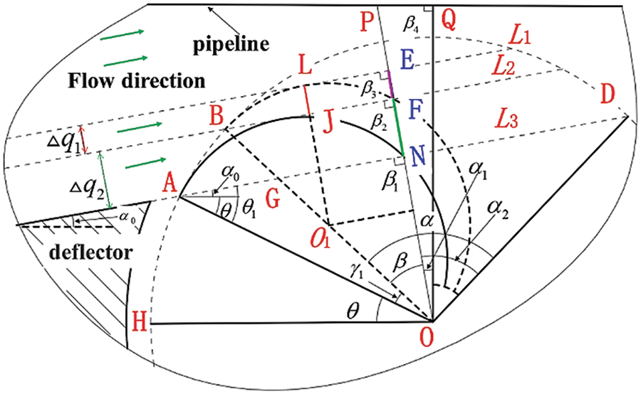
Figure 4: Coverage angle of power zone calculation diagram at B position

AG is parallel to OH, and AO=D02,β1=90∘ , then:

β=β1−(α0+θ)−γ1 (2)

OH=D02sin⁡(θ+α0) (3)

BO=D02,L2//L3,β1=β2 , then:

OF=D02cos⁡[β1−(α0+θ+γ1)] (4)

NF=D02cos⁡[β1−(α0+θ+γ1)]−D02sin⁡(θ+α0) (5)

O1L is parallel to OP through the center of the blade curvature O1, ΔBJO1≅ΔBFO , LJ=EF .

O1MOF=O1BOB (6)

MO1=D04cos⁡[β1−(α0+θ+γ1)] (7)

EF=D04−D04cos[β1−(α0+θ+γ1)] (8)

The diameter of the turbine is  D0 and the pipeline gap is δ.

OQ=D0+δ (9)

β4=90∘,OQ ⊥ OF , then:

α1=α0 (10)

PO=OQcos⁡α0 (11)

PH=OQcos⁡α0−dsin⁡(θ+α0) (12)

Under the assumption of uniform inflow, the gravity of fluid, the separation of flow, and the secondary flow were ignored in the turbine. The relationship between the fluid on the pressure and suction surface of the blade and its acting area is given by

Δq1Δq=EFPH (13)

Δq2Δq=CFPH (14)

The power torque and resistance torque of the blade are given by

M+=Δq1v(OF+EF2)cosα02 (15)

M−=Δq2v(OH+CF2)cosα02 (16)

where, v is the velocity of flow, M+ is the power moment, M− is the resistance moment.

If the resistance and power torque of the blade are equal at position B, i.e.,

M+=M− (17)

Then the relationship between the coverage angle γ1 of the main resistance zone, the turbine internal flow angle θ and the inclination angle  of deflector α0 can be written as

γ1=arcsin−1−1+10[sin2(θ+α0)+12]−5−(θ+α0) (18)

Thus, the coverage angle  α  of power zone is

α=180∘−2(α0+θ)−γ1 (19)

When the turbine internal flow angle θ and the inclination angle of deflector  α0 are determined for a hemispherical blade, the power zone coverage angle of a single blade is also determined.

As earlier mentioned, to improve the efficiency of energy utilization of the Savonius turbine, the angle of adjacent blades should be exactly equal to the angle covered by the power zone, and the optimal blade number is given by

Z≈360∘α (20)

Taking the turbine in this study as an example, it was found that Z ≈ 3.7 Therefore, the optimal number of blades of the turbine was selected as 4 in practical research.

2.3 Numerical Simulation

Basically, the internal flow field in turbomachinery is considered be complex and turbulent due to operating conditions, since it is important to choose a proper model for turbulence modeling and evaluating Navier-Stokes equations. The two-equation model [36] is a widely used turbulence model for turbomachinery numerical solving, because as the flow field of turbomachinery contains curvature and consequently is non-isotropic, more consideration should be given to the application of a two-equation model in numerical simulations for such a complex flow field. Among two-equation models, the k-ε model can offer more promise in complex flow process, and the two equations of turbulent kinetic energy (k) and turbulent dissipation rate (ε) to estimate the flow field were solved by this model. The RNG k-ε model considers the anisotropy effect of the turbulence and the rotational and swirling flow, and since the flow field inside the pipeline had a strong rotation effect, the RNG k-ε model was selected for modelling the strong rotation effect.

2.3.1 Mathematical Model

The Navier-Stokes equations [37], which are the unsteady, viscous, and incompressible turbulent flow governing equations, can be expressed in the following form:

∂ui∂xi=0 (21)

(∂ui∂t+∂∂xi(uiuj))=−∂p∂xi+∂∂xi(−ρui′uj′¯)+∂∂xj[μ(∂ui∂xj+∂uj∂xi)] (22)

where

−ρui′uj′¯=μt(∂ui∂xj+∂uj∂xi)−23(pk)δij (23)

The RNG k-ε turbulent model can be expressed in the following mathematical form:

μT=Cμρk2ε (24)

where μT is turbulent viscosity, coefficient of experience Cμ = 0.09, k is turbulent kinetic energy, ε is dissipation rate of turbulent kinetic energy.

The turbulent kinetic energy k equation:

∂∂t(ρk)+∂∂xi(ρμik)=∂∂xj[αkμeff∂k∂xj]+Gk+Gb−ρε−YM+Sk (25)

The dissipation rate of turbulent kinetic energy ε equation:

∂∂t(ρε)+∂∂xi(ρμiε)=∂∂xj[αεμeff∂ε∂xj]+C1εk(Gk+C3Gb)−C2ρε2k−Rε+Sε (26)

where C1 = 1.42, C2 = 1.68, C3 = 1.39, αk = αε = 0.7179, µeff = µ + µt and Rε are terms to adapt to the rapid flow with variable rate and streamline curvature, and its expression is:

Rε=Cuρη3(1−ηη0)1+βη3ε2k (27)

η=(Eij⋅Eij)12kε (28)

Eij=12(∂ui∂xj+∂uj∂xi) (29)

where Cµ = 0.0845, η0 = 4.38, and β = 0.012.

2.3.2 Computational Domain and Meshing

The whole computation domain is shown in Fig. 5a, which is the cylindrical section of water flow in the pipeline. To acquire the fully developed flow field, the length of the upstream inlet part was set as 6 times the diameter of the pipe, and the length of the downstream outlet part was set as 8 times the diameter of the pipe [38]. The calculation domain was divided into 4 parts, i.e., the inlet section, the deflector section, the spherical section with turbine, and the outlet section. The spherical region surrounding the turbine was defined as the rotating zone while other regions were all stationary zones. All zones were meshed with the software ICEM-CFD by polyhedral type, with the baffle tongue, leading edge and trailing edge regions refined, as shown in Fig. 5b. At the same time, there were at least 6 layers of grids in the small gap between the interface and the pipe wall, with a first layer grid height of 0.05 mm and a growth rate of 1.2.

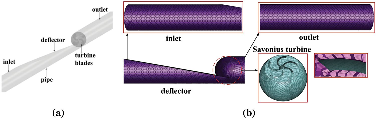
Figure 5: Computational domain and grid

2.3.3 Numerical Model and Boundary Conditions

The software ANSYS CFX18.0 was employed for the unsteady calculation, with the RNG k-ε model selected for the strong rotation effect inside the pipeline. High-precision difference scheme was adopted for the convection term, second order difference scheme was used for the diffusion term, and the SIMPLEC algorithm was applied for the coupling of velocity and pressure. Under the transient simulation, the timestep was set to 3×10−4 s corresponding to 1 degree of turbine rotation [39], and the total time was set to 1.08 s corresponding to the time needed for 10 revolutions of the turbine. The convergence condition of all residuals was the error of less than 1×10−5 under the transient simulation. The numerical result of the last rotating revolution was used for the subsequent analysis. A total pressure boundary condition was adopted at the inlet of the domain and a mass flow rate was set as the outlet boundary condition. For the wall boundaries in the calculation domain, a non-slip boundary condition was taken into consideration.

2.3.4 Verification of the Numerical Model

The grid independence verification was carried out for the numerical simulation of the Savonius hydraulic turbine with four blades. Here, the water head was selected as the variation of grid independence verification. As is shown in Fig. 6, with increasing grid number, the water head first grew quickly and then nearly leveled off when the number of grids was larger than 6.94×105 , which meant that this number of grids was sufficient to the accuracy requirement of the numerical simulation. Considering the calculation sources and time cost, the grid number of 6.94×105 was selected for the subsequent simulations.

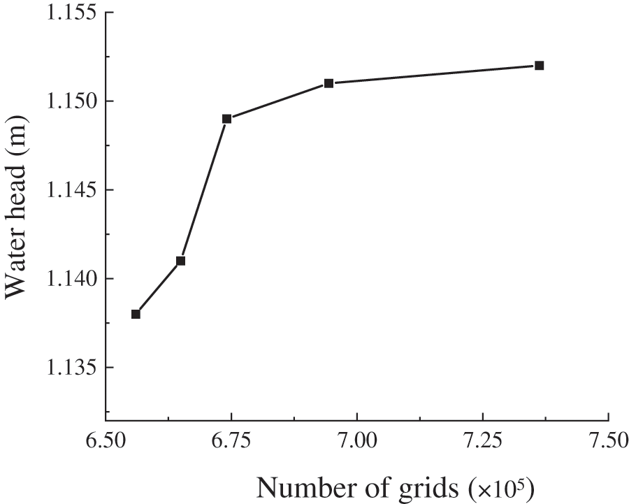
Figure 6: Grid independence verification

To verify the reliability of the numerical model, the head loss comparison between the three-dimensional simulation and experiments of the Savonius hydraulic turbine were carried out under different flow rates, as shown in Fig. 7. The results of the numerical simulation were in good agreement with those of the experiments, even when the flow rate was 5 and 6 m3/h, and the error was less than 5% (4.9% and 4.6%). Thus, the adopted CFD numerical simulation method is reasonable for the study in this paper.

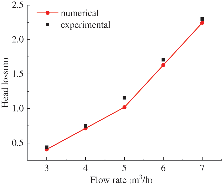
Figure 7: Comparison between CFD simulation and experiment

2.3.5 Analysis of Simulation Results

Considering that the theoretical analysis was based on the independence assumption that the inner flow velocity in the axial direction of the turbine was zero, the two-dimensional flow on the vertical plane of the central axis of the turbine was used to demonstrate the three-dimensional inner flow. To verify this assumption, the pressure contours and streamline diagrams on three slices at different vertical positions (X1, X2, X3) of the turbine are exhibited in Fig. 8, in which the flow rate was 5 m3/h and the inlet pressure was 200 kPa. The pressure distribution at different heights were very similar, so were the streamline structures. Therefore, it was feasible to replace the three-dimensional flow field of the turbine with that of the middle section, as the flow field along the axis direction of the turbine does not change much.

Figure 8: Pressure contours and streamlines of different sections

Fig. 9 shows the variation of torque on the working and back surface of a single blade at different positions. In the zone from A to B, the torque of the working surface gradually increased, while the torque of the back face gradually decreased. The resistance torque of the blade was greater than the power torque, and the blade did negative work. In the zone from B to C, the torque of the working surface increased quickly and then slightly dropped, while the torque of the back face decreased. The power torque of the blade was greater than the resistance torque, and the blade did positive work. In the zone from C to D, the torque of the working surface gradually dropped down and the torque of the back surface gradually increased. The blade still did positive work, and the power torque of the blade was greater than the resistance torque. Therefore, the B–D zone was the main energy-capturing area of the turbine in a rotation cycle. In the zone from D to A, the torque of the working surface of the blade was always smaller than that of the back face, which indicated that the resistance torque played a dominant role in this zone, and the blade did negative work. This result was consistent with the theoretical analysis.

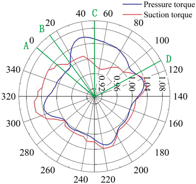
Figure 9: Torque curve

To further verify the influence of blade number on the torque of the turbine blade, the torques of blades for five groups of different blade numbers were calculated for a flow rate of 5 m3/h and an inlet pressure of 200 kPa. As shown in Fig. 10, the torques of the blades changed periodically in a rotation cycle. The less the number of blades, the greater the torque change. The area between the torque curves and the 0-point line in the figure is the average output torque in of the blade in a rotation cycle. By comparison, it was found that the average torque of the 4-blade turbine was the largest, which was consistent with the theoretical analysis.

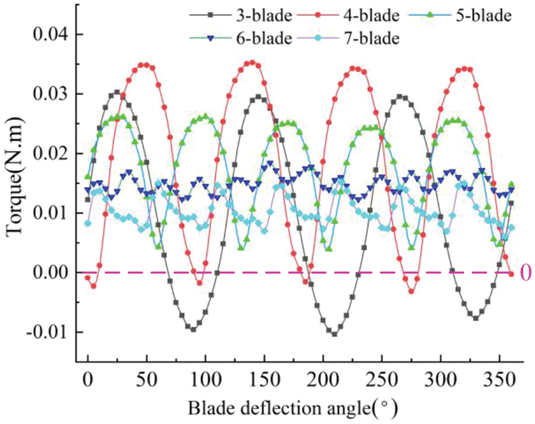
Figure 10: Turbine torque change curve of different blades

Fig. 11 displays the streamline pattern of the blade deflecting to the inter-blade region adjacent to the guide vane (as indicated by the dashed line in the figure). It was evident that for a blade count of Z = 4, the internal streamline distribution within the turbine was notably more uniform compared to turbines with other blade counts, displaying minimal inter-blade vortex formation. As the blade count increased, the streamline distribution became more chaotic, featuring distinct inter-blade vortices, resulting in a reduction in turbine efficiency. With a low blade count, the augmented fluid leakage diminished the portion of fluid impinging on the blades, subsequently diminishing the turbine’s operational effectiveness. Moreover, it was observed that a substantial high-velocity fluid existed within the gap between the pipeline and the turbine, exerting a pronounced effect on the blade tip location, thereby inducing severe torque fluctuations in the turbine.

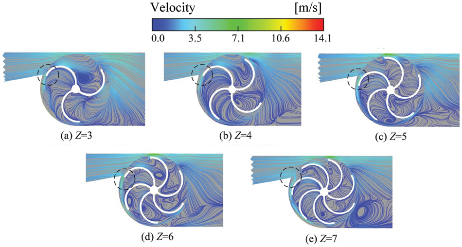
Figure 11: Streamline within the pipeline for different blade counts

2.4 Experimental Performance of the Turbine

2.4.1 Experimental Scheme

As shown in Fig. 12, the flow and head were supplied by a centrifugal pump ISG50-160 in a vertical pipe system. The experimental requirements of the turbine under different working conditions were realized by adjusting the valves at the inlet and outlet of the pump. A split electromagnetic flowmeter (ECLB50BFJ1C3DK1NV0) with an uncertainty of ± 0.5 % was installed at the inlet section to obtain the flow rate of the pipeline during the experiment. Two manometers (JT118) with an uncertainty of ± 0.5 % were installed at the inlet and outlet of the pipe section respectively to obtain the pressure of the inlet and outlet. A tachometer (VC6236P) with an uncertainty of ± 0.5 % was used to obtain the rotation speed of turbine. The output shaft of the turbine was connected to a generator which could output direct current (DC) by using a rectifier. Considering that the shaft power generated by the turbine was small and was difficult to measure, the current and voltage of the generator were measured, and the electric power was calculated to replace the shaft power. As depicted in Fig. 13, the turbine is fabricated using photosensitive resin material, and for comparative analysis, five different scenarios are considered with varying blade numbers (Z) set at 3, 4, 5, 6, and 7. Importantly, all other operational parameters and conditions are held constant across these scenarios for consistency and accuracy in the assessment. The efficiency of energy conversion of the turbine is given by

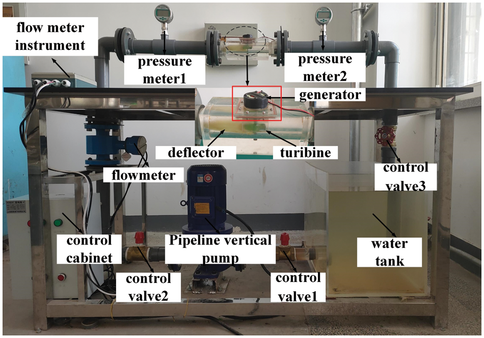
Figure 12: Pipeline Savonius hydraulic turbine experiment system

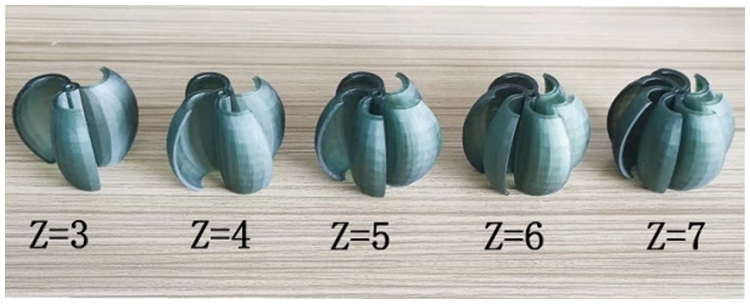
Figure 13: Turbines with different blades

η=PelectricityQ(Pin−Pout) (30)

where Pelectricity is the output electrical power of the generator, Q is the flow rate of the pipeline, Pin is the pressure at the inlet of the pipeline, Pout is the pressure at the outlet of the pipeline.

2.4.2 Analysis of Experimental Results

The rotating speed/water head–flow rate curve is shown in Fig. 14. The water head variation trend at different sections of the turbine was similar. The rotating speed of the turbine increased linearly with increasing flow rate, and the differences in the rotating speed between the different blade numbers were close. Obviously, the turbine with four blades exhibited the fastest rotating speed. Similarly, the water head difference increased with increasing flow rate. When the flow rate was between 4 and 6 m3/h, the water head exhibited a big difference between different blade numbers.

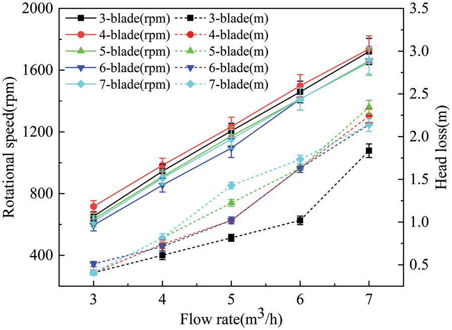
Figure 14: Rotating speed/water head-flow rate curves

The electric power-flow rate curves are shown in Fig. 15. The electrical power of the 4-blade turbine was the highest and that of the 3-blade turbine was the lowest. With increasing flow rate and rotating speed, the voltage and current of the generator, and the electrical power increased slowly. While the differences of voltage and current between the different blade number were close, when the flow rate was 5 m3/h, the output power of the 4-blade turbine was lower than that of other blades number of turbines. Under such conditions, the turbine slipped on the shaft, the voltage of the generator was unstable, and the rotating speed electrical power decreased.

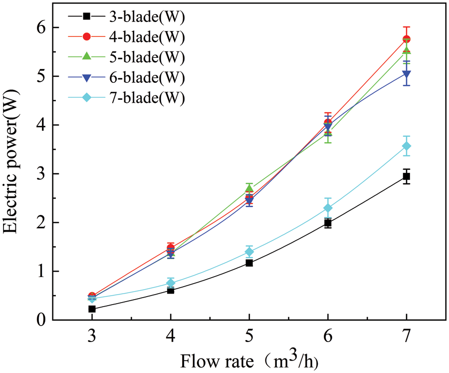
Figure 15: Electric power-flow rate curves

The efficiency-flow rate curves are shown in Fig. 16. With increasing flow rate, the efficiency of the turbine first increased and then decreased, in which the turbine with four blades exhibited the highest efficiency (peak of 19.05%). This was because at the same rotating speed, the turbine with four blades could obtain the maximum torque within a rotation cycle (namely the maximum fluid power), which was the main reason for its high efficiency. In addition, on the one hand, there were too many blades in the power zone at the same time, the returning blade influenced the incoming flow working on the advancing blade, resulting in the decrease of the effective area of the blade and the decrease of the incoming flow energy. On the other hand, the hydraulic loss increased with increasing flow velocity and extrusion in the turbine channel. However, for the cases of small blade number, the constraint ability of the blade on the fluid decreased, the velocity slip was more serious, thus the working ability of the blade decreased and the additional hydraulic loss increased [40].

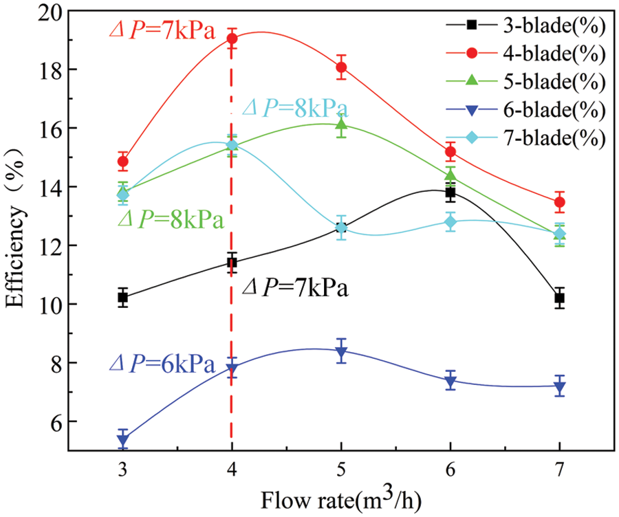
Figure 16: Efficiency-flow rate curves

3  Economic Benefit Prediction

The device which is the research object in this study has already been successfully applied in the process of energy recovery. Taking Chinese Lanzhou New Area as an example, the local area pipeline network layout is shown in Fig. 17. The range from south to north is 100–200 m. Water supply companies located at the upstream region provide the downstream users with water resource based on the geographical disparity. The partial pressure is up to 0.5–0.9 MPa. To ensure normal water supply for residents, a pressure reducing valve is installed in partial regions to reduce the water pressure, and the excess pressure energy of fluid after depressurization is usually wasted directly. Therefore, how to take full advantage of the energy of fluid to reduce pressure is an urgent problem for companies. According to investigation, lithium batteries are used for the pressure and flow monitoring equipment in the water supply network. This monitoring equipment updates data every 10 min, which requires a high performance of the battery. Nowadays, the batteries used in the equipment need to be replaced frequently since its life is limited to about 1–3 months in summer and 7 days in winter, which substantially increases cost and environmental pollution. If the Savonius hydraulic turbine is installed in pipes of different diameters to recovery energy, then the device turbine will be driven by the excess pressure of water and generate electricity for the pipeline data acquisition system. The social resources will be saved and the ecological environment will be protected to a large extent.

Figure 17: Local area pipeline network layout

The schematic of the proposed system is shown in Fig. 18. The water supply network of DN50 in a certain area of the Chinese Lanzhou New Area was selected to analyze the economic benefits of the newly proposed system.

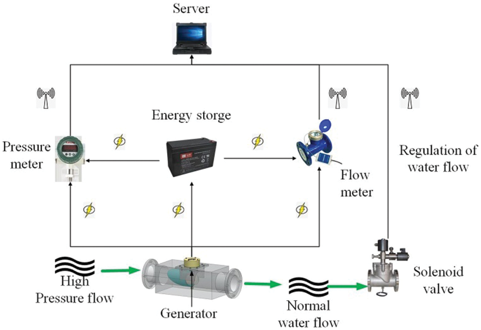
Figure 18: Savonius hydraulic turbine system power generation device

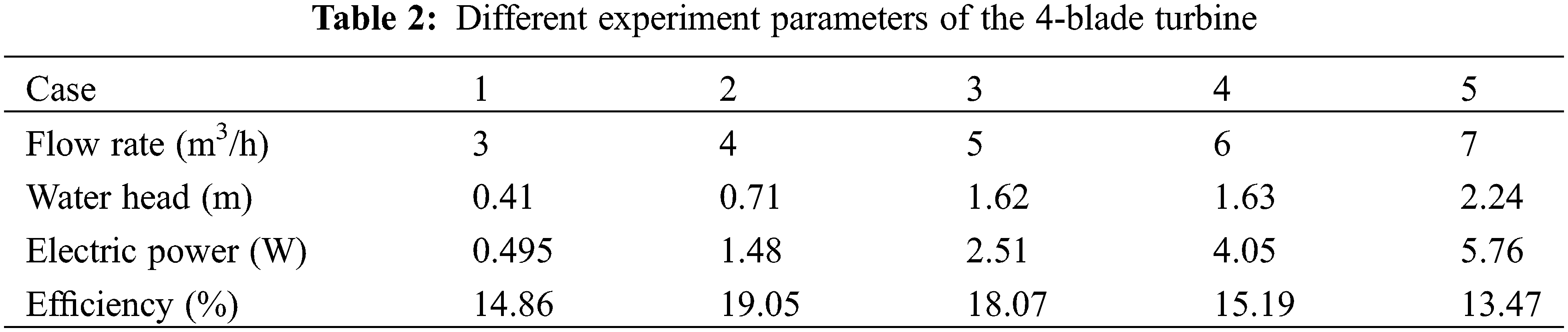
Table 2 provides a comprehensive list of the diverse experimental parameters that pertain to the performance assessment of the 4-blade turbine. These parameters encapsulate a range of cases, each distinguished by distinct flow rates and corresponding water head values. Subsequently, a meticulous analysis of this dataset follows, aimed at discerning salient trends and implications. The individual cases, designated as 1 through 5, spanned a continuum of flow rates from 3 to 7 m³/h, coupled with varying water head measurements ranging from 0.41 to 2.24 m. These parameters bear intricate relationships with two critical performance metrics: electric power output, measured in watts (W), and turbine efficiency, denominated in percentage (%). An inherent pattern became evident upon dissecting the interplay between flow rate, water head, electric power output, and efficiency. Particularly noteworthy was Case 2, characterized by a flow rate of 4 m³/h and a corresponding water head of 0.71 m. This configuration registered a remarkable advancement in both electric power output, reaching 1.48 W, and efficiency, achieving 19.05%. Similar observations were drawn from Case 3, where a flow rate of 5 m³/h and a water head of 1.62 m manifested in an electric power output of 2.51 W and an efficiency of 18.07%. Conversely, as flow rate and water head dimensions expanded in Cases 4 and 5, the electric power output experienced proportional escalation, peaking at 4.05 W for Case 4 and 5.76 W for Case 5. However, the efficiency metric portrayed a more intricate trajectory. Case 4 exhibited a slight decrement in efficiency, registering at 15.19%, while Case 5 materialized with the lowest efficiency of the examined cases, at 13.47%.

As is known, the efficiency and water head of a Savonius hydraulic turbine are basic parameters to measure its hydraulic performance. It was found that the water head linearly increased with increasing flow rate, as shown in Fig. 19, and the fitted relationship is given by

Figure 19: Fitting curve of flow rate and water head

H=(0.43Q−1.1) (31)

where Q is the flow rate of pipeline, H is the water head of pipeline. However, there was a cubic relationship between the efficiency and the flow rate, as shown in Fig. 20, and the fitted relationship is given by

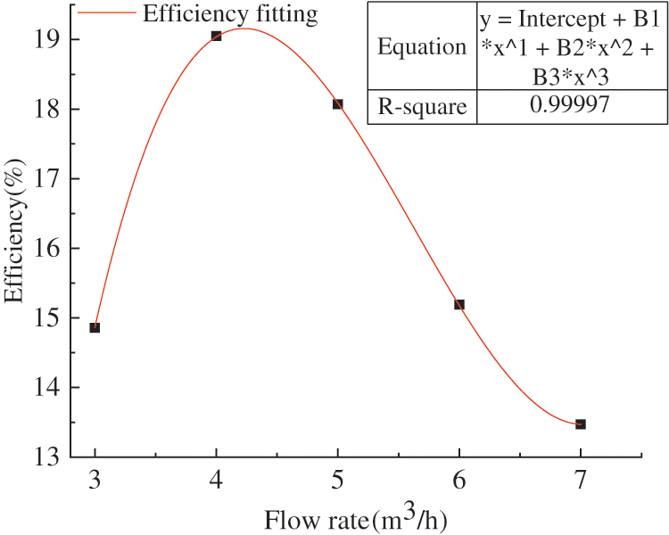
Figure 20: Fitting curve of flow rate and efficiency

η=(0.5275Q3−8.8925Q2+46.905Q−60.062) (32)

where η is the efficiency of the Savonius hydraulic turbine.

The seasonal proportion of water supply and its monthly flow rate in the Lanzhou New Area in 2020 are shown in Figs. 21 and 22, respectively. The peak of water consumption was mainly concentrated in summer, and the trough in winter. More water was used in May and less in December. The water consumption on a certain day in May and December were selected to analyze the power generation of the device with different flow rates on these days. The daily water supply distribution is shown in Figs. 23 and 24. Taking one day as example, the economic benefit of the device of DN50 pipe diameter in one year was calculated.

Figure 21: Seasonal distribution of water supply

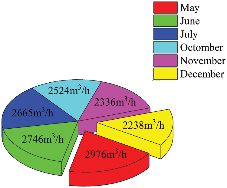
Figure 22: Monthly distribution of water supply

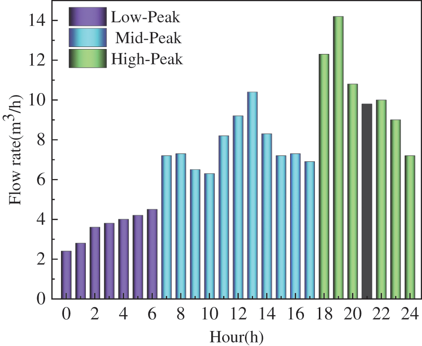
Figure 23: Water supply on May 12

Figure 24: Water supply on December 10

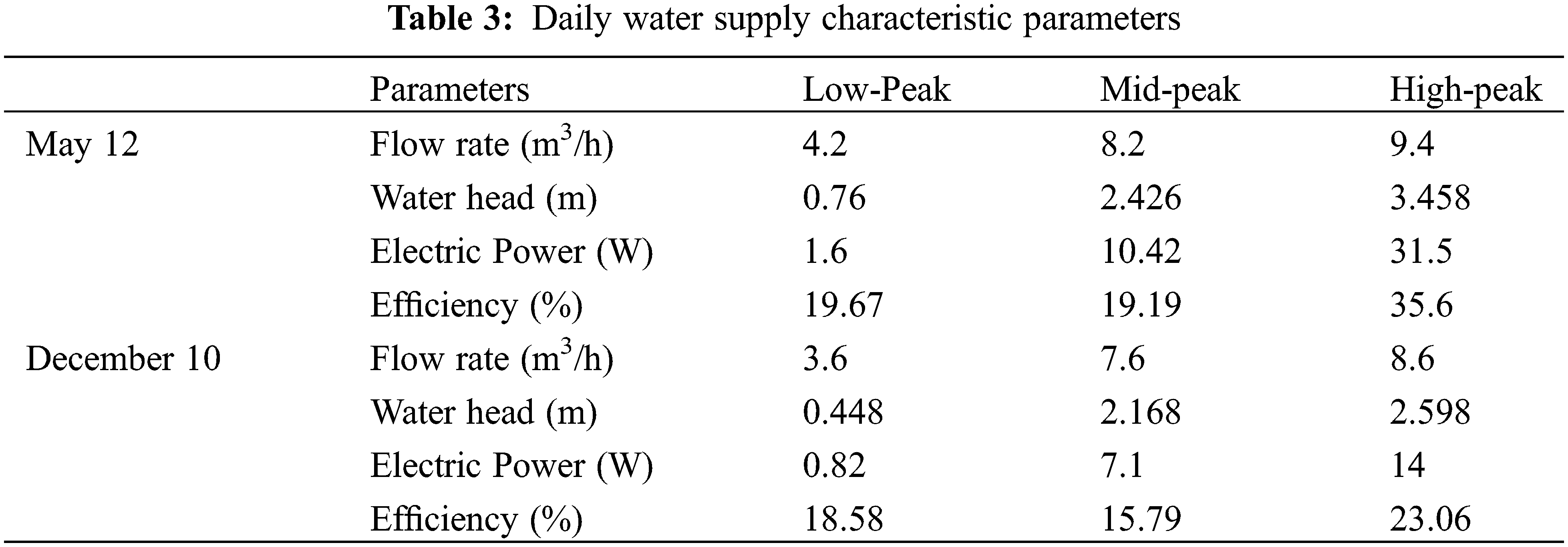
As is shown in Figs. 22 and 23, the trends of water consumption in May and December were consistent, which could be divided into the low-peak period from 12 a.m. to 6 a.m., the mid-peak period from 7 a.m. to 5 p.m. and the high-peak period from 6 p.m. to midnight. To obtain accurate results, the average water consumption of the different periods were selected to calculate the power generation of the device at the given flow rate. The performance parameters of the Savonius hydraulic turbine under different flow rates are presented in the Table 3, in which the water head and efficiency were obtained according to Eqs. (31) and (32). The parameters of the power supply specifications of some remote transmission equipment are presented in Table 4.

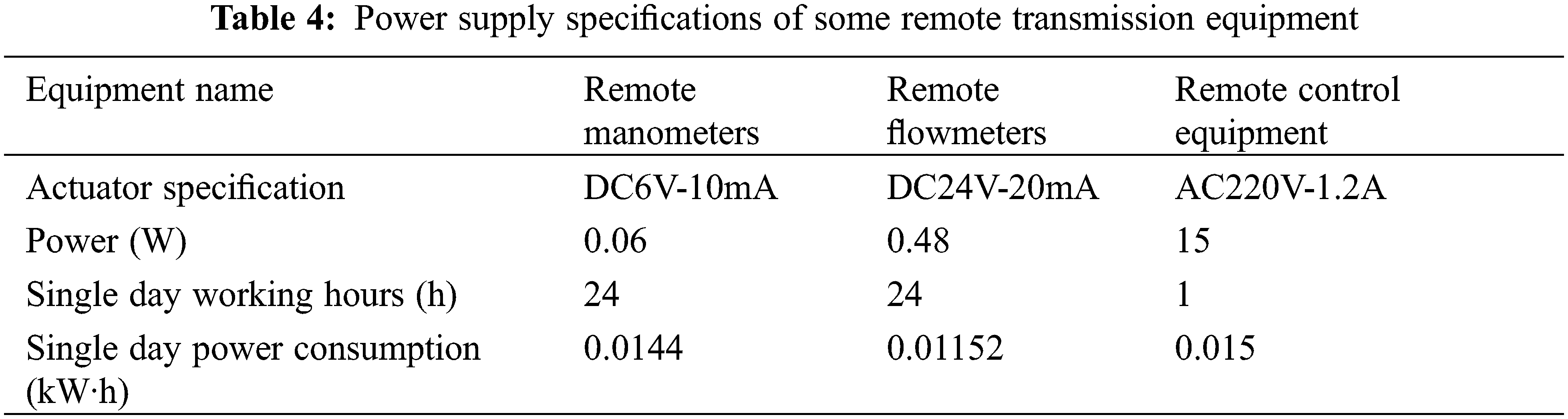
From Table 4, it is obvious that the operational timeframe of remote-control equipment within the pipeline network spanned a range of 26 to 100 s, with a daily operational duration of 1 to 2 h. Notably, the continuous transmission of data from the remote manometers and flowmeters operated around the clock. It is imperative to acknowledge the seasonal influence, which significantly shaped the energy demands of these monitoring devices. During the summer months, under normal operating conditions, the flowmeters and manometers at a singular node required a complement of 8 batteries to ensure consistent functionality. In precise terms, the flowmeters required battery replacement every 21 days, while the manometers required new batteries every 30 days. Furthermore, the remote-control equipment consumed approximately 1.8 kW·h of electricity daily. Winter introduced a more demanding scenario due to lowered temperatures and aggravated battery performance. Consequently, the flowmeters required battery replacement every 9 days, and the manometers required new batteries every 15 days. This operational paradigm, while sustaining the equipment, unfortunately contributed to a proliferation of lithium batteries, thereby engendering environmental degradation. A promising alternative solution was exemplified by the integration of the Savonius hydraulic turbine within the pipeline infrastructure to provide electricity for the monitoring equipment. In this context, the turbine exhibited impressive capability, generating 0.313 kW·h of electricity over a 24 h cycle during summer. To elucidate, this was distributed as 0.114 kW·h during low-peak periods, 1.518 kW·h during mid-peak periods, and another 0.114 kW·h during high-peak periods. Transitioning to the winter scenario, the turbine generated 0.167 kW·h over 24 h, encompassing 0.0049 kW·h during low-peak hours, 0.078 kW·h during mid-peak hours, and 0.084 kW·h during high-peak hours. Consequently, the installation of the Savonius hydraulic turbine at a singular node achieved a seamless power supply for the two remote control valves, two flowmeters, and two manometers throughout the day and night, both in summer and winter, without encroaching upon water supply functionality. This transformative solution heralds promising outcomes, alleviating battery dependency, mitigating environmental repercussions, and ensuring the sustained operation of critical monitoring equipment. The culmination of these benefits is succinctly summarized in the annual cost comparison as shown in Table 5.

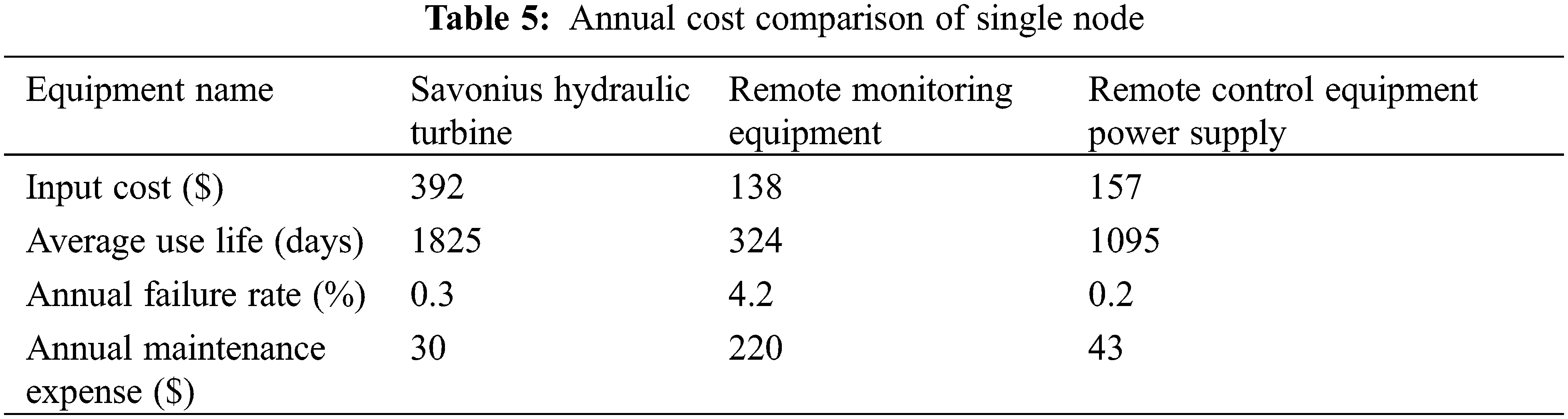
As presented in Table 5, the input cost of single node the remote transmission equipment was much lower than that of the Savonius hydraulic turbine in the pipeline network. However, the batteries need to be replaced twice per month for the flowmeters and once per month for the manometers in summer. A total of 36 batteries were needed for the monitoring equipment every month. In accordance with the prevailing market price of a battery, the annual battery expense is about $105. In winter, the number of batteries was doubled, so the annual battery expense was $210. In addition, the labor costs increased due to the frequent replacement of batteries. The remote transmission control equipment needed to consume 54.75 kW·h of electricity energy every year. In accordance with the prevailing electricity price, $30 needed to be paid. To sum up, a single node costs about $658 every year. With 15 monitoring nodes in this area, this translated to a cost of about $8408 every year. In contrast, the Savonius hydraulic turbine required only one-time manufacturing and installation costs, with the average annual life span being significantly higher than that of the conventional battery-powered devices. Only 15 devices were required in the area to meet the power supply requirements of 15 nodes, and it took only half of a year to balance the receipts and payments. In terms of power generation, the Savonius hydraulic turbine could generate 28.17 kW·h electricity energy in summer and 15.03 kW·h electricity energy in winter within one day, which was enough for the system. Besides, about 200 lithium batteries in a single node were consumed each year and 3000 lithium batteries are consumed for 15 nodes, for which the disposal of the spent batteries caused serious environmental pollution. The remote transmission equipment needed 0.15 kW·h electricity energy to work for 1 h, which was equivalent to the annual emission of 54.75 kg CO2. Thus, the Savonius hydraulic turbine, as a clean energy recovery device could generate 86.4 kW·h, which could result in a reduction of about 111.8 kg CO2 emissions every year.

4  Conclusion

In this paper, a Savonius turbine which was used for micro power generation in a water pipeline system was studied theoretically, experimentally, and numerically. The turbine with a deflector was directly installed in the water pipeline system to supply data monitoring system. Experiments were carried out to verify the numerical simulation, and the effect of blade number on the torque and efficiency of turbine were investigated by numerical simulation. Moreover, based on the external characteristic parameters of the optimal number of blades turbine, the application of the devices was analyzed to predict its energy saving efficiency and economic benefits. The main results are as follows:

1.    The variation of torque of the Savonius turbine in a rotation period could be divided into 4 zones: main resistance zone, main power zone, secondary power zone and secondary resistance zone. The main power zone and the secondary power zone were the zones of positive torque, and the main resistance zone and the secondary resistance zone were the zones of negative torque.

2.    The analytical relationship between the coverage angle α of the power zone, the internal flow angle θ and the angle of deflector α0 were established based on the maximum power zone. A calculation method for the optimal number of blades was proposed. Based on this method, the calculated optimal number of blades in this study was four. The power experiments on five groups of turbines with 3-, 4-, 5-, 6-, and 7-blades showed that both the recovery power and efficiency of the turbine were the highest (5.76 W and 19.05%, respectively) when the blade number was 4, which showed that the calculation method of the number of optimal blades proposed in this paper is valid.

3.    With increasing flow rate, both the rotating speed and pressure difference of the Savonius turbine increased linearly, and the power increased slowly at first and then rapidly dropped. The increase of blade number was related to the decrease of the torque variation.

4.    Taking the DN50 pipeline system in a certain area as an example, it was found that the use of the Savonius turbine can generate electricity energy of 28.17 kW·h in summer and 15.03 kW·h in winter. This would save about $593 in a year for a single node, and total savings in this area (for 15 nodes) of about $8408. Meanwhile, application of the device can reduce about 111.8 kg CO2 of emissions each year, and can reduce about 200 lithium batteries for a single node. Thus, the purpose of energy saving and emission reduction is realizable using this system.

Acknowledgement: None.

Funding Statement: This research was funded by Gansu Outstanding Youth Fund (20JR10RA203), Gansu Province Youth Doctor Fund (2023QB-033), National Natural Science Foundation of China (52169019) and the Gansu Industry-University Support Fund (2020C-20).

Author Contributions: The authors confirm contribution to the paper as follows: study conception and design: Xiaohui Wang, Kai Zhang; data collection: Kai Zhang, Zanxiu Wu; analysis and interpretation of results: Xiaohui Wang, Kai Zhang, Xiaobang Bai, Senchun Miao; draft manuscript preparation: Kai Zhang, Xiaohui Wang, Zanxiu Wu, Jicheng Li. All authors reviewed the results and approved the final version of the manuscript.

Availability of Data and Materials: Not applicable.

Conflicts of Interest: The authors declare that they have no conflicts of interest to report regarding the present study.

References

1. Mazzolani, G., Berardi, L., Laucelli, D. B., Simone, A., Martino, R. et al. (2017). Estimating leakages in water distribution networks based only on inlet flow data. Journal of Water Resources Planning and Management, 143(6), 1–11. https://doi.org/10.1061/(asce)wr.1943-5452.0000758 [Google Scholar] [CrossRef]

2. Xu, Q., Liu, R., Chen, Q., Li, R. (2014). Review on water leakage control in distribution networks and the associated environmental benefits. Journal of Environmental Sciences, 26(5), 955–961. https://doi.org/10.1016/s1001-0742(13)60569-0 [Google Scholar] [PubMed] [CrossRef]

3. Ma, T., Yang, H., Lu, L. (2014). A feasibility study of a stand-alone hybrid solar-wind–battery system for a remote island. Applied Energy, 121, 149–158. https://doi.org/10.1016/j.apenergy.2014.01.090 [Google Scholar] [CrossRef]

4. Ma, T., Yang, H., Lu, L. (2014a). Feasibility study and economic analysis of pumped hydro storage and battery storage for a renewable energy powered island. Energy Conversion and Management, 79, 387–397. https://doi.org/10.1016/j.enconman.2013.12.047 [Google Scholar] [CrossRef]

5. Niyato, D., Hossain, E., Rashid, M., Bhargava, V. K. (2007). Wireless sensor networks with energy harvesting technologies: A game-theoretic approach to optimal energy management. IEEE Wireless Communications, 14(4), 90–96. https://doi.org/10.1109/mwc.2007.4300988 [Google Scholar] [CrossRef]

6. Ma, T., Yang, H., Lu, L. (2015). Study on stand-alone power supply options for an isolated community. International Journal of Electrical Power & Energy Systems, 65, 1–11. https://doi.org/10.1016/j.ijepes.2014.09.023 [Google Scholar] [CrossRef]

7. Casini, M. (2015). Harvesting energy from in-pipe hydro systems at urban and building scale. International Journal of Smart Grid and Clean Energy, 4(4), 316–327. https://doi.org/10.12720/sgce.4.4.316-327 [Google Scholar] [CrossRef]

8. Du, J. Y., Yang, H. X., Shen, Z. C., Guo, X. D. (2018). Development of an inline vertical cross-flow turbine for hydropower harvesting in urban water supply pipes. Renewable Energy, 127, 386–397. https://doi.org/10.1016/j.renene.2018.04.070 [Google Scholar] [CrossRef]

9. Rosenbloom, D. I. S., Meadowcroft, J. (2014). Harnessing the Sun: Reviewing the potential of solar photovoltaics in Canada. Renewable & Sustainable Energy Reviews, 40, 488–496. https://doi.org/10.1016/j.rser.2014.07.135 [Google Scholar] [CrossRef]

10. Dondi, D., Bertacchini, A., Brunelli, D., Lugli, P., Benini, L. (2008). Modeling and optimization of a solar energy harvester system for self-powered wireless sensor networks. IEEE Transactions on Industrial Electronics, 55(7), 2759–2766. https://doi.org/10.1109/tie.2008.924449 [Google Scholar] [CrossRef]

11. Park, J. C., Jung, H., Jo, H., Jang, S., Spencer, B. F. (2010). Feasibility study of wind generator for smart wireless sensor node in cable-stayed bridge. Proceedings of Sensors and Smart Structures Technologies for Civil, Mechanical, and Aerospace Systems 2010, San Diego, USA. https://doi.org/10.1117/12.853600 [Google Scholar] [CrossRef]

12. Xia, R., Farm, C., Choi, W., Kim, S. (2006). Self-powered wireless sensor system using MEMS piezoelectric micro power generator. 5th IEEE Sensors Conference, Daegu, South Korea. https://doi.org/10.1109/icsens.2007.355704 [Google Scholar] [CrossRef]

13. Sun, J., Hu, J. (2011). Experimental study on a vibratory generator based on impact of water current. 2011 Symposium on Piezoelectricity, Acoustic Waves and Device Applications (SPAWDA), Shenzhen, China. https://doi.org/10.1109/spawda.2011.6167186 [Google Scholar] [CrossRef]

14. Jaohindy, P., McTavish, S., Garde, F., Bastide, A. (2013). An analysis of the transient forces acting on Savonius rotors with different aspect ratios. Renewable Energy, 55, 286–295. https://doi.org/10.1016/j.renene.2012.12.045 [Google Scholar] [CrossRef]

15. Mosbahi, M., Derbel, M., Lajnef, M., Mosbahi, B., Driss, Z. et al. (2021). Performance study of twisted darrieus hydrokinetic turbine with novel blade design. Journal of Energy Resources, 143(9), 091302. https://doi.org/10.1115/1.4051483 [Google Scholar] [CrossRef]

16. Yang, W., Hou, Y., Jia, H., Liu, B., Xiao, R. (2019). Lift-type and drag-type hydro turbine with vertical axis for power generation from water pipelines. Energy, 188, 116070. https://doi.org/10.1016/j.energy.2019.116070 [Google Scholar] [CrossRef]

17. Maldar, N. R., Ng, C. H., Oguz, E. (2020b). A review of the optimization studies for Savonius turbine considering hydrokinetic applications. Energy Conversion and Management, 226, 113495. https://doi.org/10.1016/j.enconman.2020.113495 [Google Scholar] [CrossRef]

18. Kamoji, M. A., Kedare, S. B., Prabhu, S. (2008). Experimental investigations on single stage, two stage and three stage conventional Savonius rotor. International Journal of Energy Research, 32(10), 877–895. https://doi.org/10.1002/er.1399 [Google Scholar] [CrossRef]

19. Basumatary, M., Biswas, A., Misra, R. D. (2020). Detailed hydrodynamic study for performance optimization of a combined lift and drag-based modified savonius water turbine. Journal of Energy Resources, 142(8), 081301. https://doi.org/10.1115/1.4045924 [Google Scholar] [CrossRef]

20. Mosbahi, M., Ayadi, A., Chouaibi, Y., Driss, Z., Tucciarelli, T. (2019). Performance study of a Helical Savonius hydrokinetic turbine with a new deflector system design. Energy Conversion and Management, 194, 55–74. https://doi.org/10.1016/j.enconman.2019.04.080 [Google Scholar] [CrossRef]

21. Patel, V., Bhat, G., Eldho, T. I., Prabhu, S. (2017). Influence of overlap ratio and aspect ratio on the performance of Savonius hydrokinetic turbine. International Journal of Energy Research, 41(6), 829–844. https://doi.org/10.1002/er.3670 [Google Scholar] [CrossRef]

22. Yao, J., Li, F., Chen, J., Yuan, Z., Mai, W. (2019). Parameter analysis of savonius hydraulic turbine considering the effect of reducing flow velocity. Energies, 13(1), 24. https://doi.org/10.3390/en13010024 [Google Scholar] [CrossRef]

23. Kumar, A., Saini, R. (2017b). Performance analysis of a Savonius hydrokinetic turbine having twisted blades. Renewable Energy, 108, 502–522. https://doi.org/10.1016/j.renene.2017.03.006 [Google Scholar] [CrossRef]

24. Kerikous, E., Thévenin, D. (2019). Optimal shape of thick blades for a hydraulic Savonius turbine. Renewable Energy, 134, 629–638. https://doi.org/10.1016/j.renene.2018.11.037 [Google Scholar] [CrossRef]

25. Talukdar, P. K., Kulkarni, V., Saha, U. K. (2018). Performance estimation of Savonius wind and Savonius hydrokinetic turbines under identical power input. Journal of Renewable and Sustainable Energy, 10(6), 064704. https://doi.org/10.1063/1.5054075 [Google Scholar] [CrossRef]

26. Zhou, Q., Xu, Z., Cheng, S., Huang, Y., Xiao, J. (2018). Innovative Savonius rotors evolved by genetic algorithm based on 2D-DCT encoding. Soft Computing, 22(23), 8001–8010. https://doi.org/10.1007/s00500-018-3214-x [Google Scholar] [CrossRef]

27. Golecha, K., Eldho, T. I., Prabhu, S. (2011). Influence of the deflector plate on the performance of modified Savonius water turbine. Applied Energy, 88(9), 3207–3217. https://doi.org/10.1016/j.apenergy.2011.03.025 [Google Scholar] [CrossRef]

28. Salleh, M. A. A. M., Kamaruddin, N. M., Mohamed-Kassim, Z. (2021). The effects of a deflector on the self-starting speed and power performance of 2-bladed and 3-bladed Savonius rotors for hydrokinetic application. Energy for Sustainable Development, 61, 168–180. https://doi.org/10.1016/j.esd.2021.02.005 [Google Scholar] [CrossRef]

29. Yao, Y., Tang, Z., Wang, X. F. (2013). Design based on a parametric analysis of a drag driven VAWT with a tower cowling. Journal of Wind Engineering and Industrial Aerodynamics, 116, 32–39. https://doi.org/10.1016/j.jweia.2012.11.001 [Google Scholar] [CrossRef]

30. Thakur, N. S., Biswas, A., Kumar, Y., Basumatary, M. (2019). CFD analysis of performance improvement of the Savonius water turbine by using an impinging jet duct design. Chinese Journal of Chemical Engineering, 27(4), 794–801. https://doi.org/10.1016/j.cjche.2018.11.014 [Google Scholar] [CrossRef]

31. Elbatran, A. H., Ahmed, Y. M., Shehata, A. Z. (2017b). Performance study of ducted nozzle Savonius water turbine, comparison with conventional Savonius turbine. Energy, 134, 566–584. https://doi.org/10.1016/j.energy.2017.06.041 [Google Scholar] [CrossRef]

32. Payambarpour, S. A., Najafi, A. A., Magagnato, F. (2020). Investigation of deflector geometry and turbine aspect ratio effect on 3D modified in-pipe hydro Savonius turbine: Parametric study. Renewable Energy, 148, 44–59. https://doi.org/10.1016/j.renene.2019.12.002 [Google Scholar] [CrossRef]

33. Chen, J. C., Yang, H., Liu, C., Lau, C. S., Lo, M. (2013). A novel vertical axis water turbine for power generation from water pipelines. Energy, 54, 184–193. https://doi.org/10.1016/j.energy.2013.01.064 [Google Scholar] [CrossRef]

34. Layeghmand, K., Tabari, N. G., Zarkesh, M. (2020). Improving efficiency of savonius wind turbine by means of an airfoil-shaped deflector. Journal of the Brazilian Society of Mechanical Sciences and Engineering, 42(10), 801–818. https://doi.org/10.1007/s40430-020-02598-7 [Google Scholar] [CrossRef]

35. Golecha, K., Eldho, T. I., Prabhu, S. (2012). Performance study of modified savonius water turbine with two deflector plates. International Journal of Rotating Machinery, 2012, 1–12. https://doi.org/10.1155/2012/679247 [Google Scholar] [CrossRef]

36. Mompean, G. (1998). Numerical simulation of a turbulent flow near a right-angled corner using the Speziale non-linear model with RNG K–ε equations. Computers & Fluids, 27(7), 847–859. https://doi.org/10.1016/s0045-7930(98)00004-8 [Google Scholar] [CrossRef]

37. Thomas, T. Y. (1943). On the uniform convergence of the solutions of the navier-stokes equations. Proceedings of the National Academy of Sciences of the United States of America, 29(8), 243–246. https://doi.org/10.1073/pnas.29.8.243 [Google Scholar] [PubMed] [CrossRef]

38. Mauro, S., Brusca, S., Lanzafame, R., Messina, M. (2019). CFD modeling of a ducted Savonius wind turbine for the evaluation of the blockage effects on rotor performance. Renewable Energy, 141, 28–39. https://doi.org/10.1016/j.renene.2019.03.125 [Google Scholar] [CrossRef]

39. Shaheen, M. F., El-Sayed, M., Abdallah, S. (2015). Numerical study of two-bucket Savonius wind turbine cluster. Journal of Wind Engineering and Industrial Aerodynamics, 137, 78–89. https://doi.org/10.1016/j.jweia.2014.12.002 [Google Scholar] [CrossRef]

40. Wang, X. (2018). Research on slip phenomenon of pumps as turbines. Jixie Gongcheng Xuebao, 54(24), 189–196 (In Chinese). https://doi.org/10.3901/jme.2018.24.189 [Google Scholar] [CrossRef]