
 Submit a Paper
 Propose a Special lssue
 Open Access
ARTICLE
Evaluation of Well Spacing for Primary Development of Fractured Horizontal Wells in Tight Sandstone Gas Reservoirs
1 Exploration and Development Research Institute, PetroChina Southwest Oil & Gas Field Company, Chengdu, 610041, China
2 Oil and Gas Resources Department, PetroChina Southwest Oil & Gas Field Company, Chengdu, 610000, China
* Corresponding Author: Fang Li. Email:
(This article belongs to the Special Issue: Solid, Fluid, and Thermal Dynamics in the Development of Unconventional Resources )
Fluid Dynamics & Materials Processing 2024, 20(5), 1015-1030. https://doi.org/10.32604/fdmp.2023.043256
Received 27 June 2023; Accepted 21 November 2023; Issue published 07 June 2024
 View Full Text
 Download PDF
Abstract
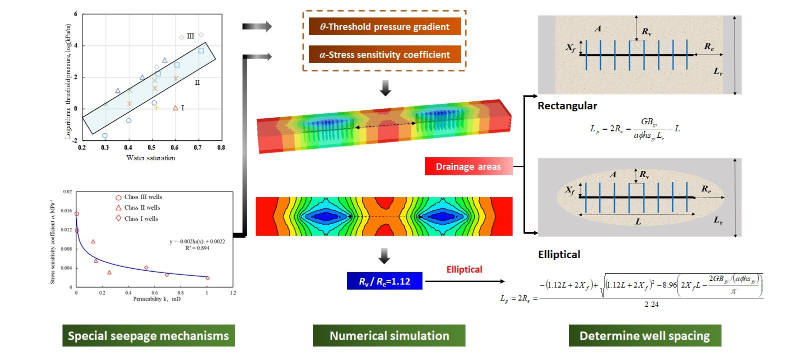
Methods for horizontal well spacing calculation in tight gas reservoirs are still adversely affected by the complexity of related control factors, such as strong reservoir heterogeneity and seepage mechanisms. In this study, the stress sensitivity and threshold pressure gradient of various types of reservoirs are quantitatively evaluated through reservoir seepage experiments. On the basis of these experiments, a numerical simulation model (based on the special seepage mechanism) and an inverse dynamic reserve algorithm (with different equivalent drainage areas) were developed. The well spacing ranges of Classes I, II, and III wells in the Q gas field are determined to be 802–1,000, 600–662, and 285–400 m, respectively, with their average ranges as 901, 631, and 342.5 m, respectively. By considering both the pairs of parallel well groups and series well groups as examples, the reliability of the calculation results is verified. It is shown that the combination of the two models can reduce errors and provide accurate results.Graphic Abstract
Keywords
Nomenclature
| | Stress sensitivity coefficient, decimal |
| k | Permeability, mD |
| ϕ | Porosity, decimal |
| Sw | Water saturation, decimal |
| Sg | Gas saturation, decimal |
| θ | Threshold pressure gradient, kPa/m |
| L | Horizontal segment length, m |
| Lr | Channel width, m |
| pi | Initial pressure, MPa |
| ki | Initial permeability, mD |
| kr | Relative permeability, decimal |
| T | Temperature, °C |
| n | Fracturing segments |
| Xf | Fracture half-length, m |
| A | Control area, m2 |
| h | Reservoir thickness, m |
| G | Dynamic reserves, m3 |
| Bgi | Volume factor, m3/m3 |
| Sgi | Original gas saturation, decimal |
| Re | Extrapolation distance, m |
| Rv | Radial extrapolation distance, m |
| qg | Open flow, 104m3/d |
| V | Velocity, m3/s |
| μ | Viscosity, mPa∙s |
The Securities and Exchange Commission (SEC) reserve is a petroleum reserve calculated and disclosed by oil and gas companies listed in the US in accordance with the rules of the US SEC [1–3]. The SEC reserve is critical in exploration, development, production, and operation processes; the evaluation results are required to have reasonable certainty to ensure minimum risks for investors. SEC reserve estimation has become a key index in the production and management assessment of oil and gas companies listed in the US. The requirements for SEC reserve estimation are becoming more stringent yearly [4–8]. For wells in the early development stage, a volumetric method is generally used for SEC reserve estimation. Owing to the uncertain input parameters used to calculate SEC reserves, a combination of parameters can magnify the error in the estimation results [9–11]. Well spacing for primary development, which can be determined by analogy or dynamic reserve calculation to reduce the estimation error, is one of the decisive factors in reserve estimation using a volumetric method [12–14].
At present, analogy and an inverse dynamic reserve algorithm are widely used to calculate well control ranges [15–18]. The analogy method is applied by selecting gas reservoirs with similar geological and engineering conditions to determine the well spacing of target gas reservoirs. The inverse dynamic reserve algorithm is based on the inverse dynamic reserve calculation of a drainage area to determine well spacing. This combined with the well control range and length of a horizontal well, well spacing for primary development can be determined. When searching for gas reservoirs with similar geological and engineering conditions, the well control range can only be qualitatively evaluated using the analogy method, as many experiments have shown that percolation in low permeability does not fit Darcy’s Law [19–22]. Ning et al. [23] reported that fluid flowing in a tight reservoir must overcome the resistance exerted by the adsorption or hydration film formed in the reservoir. The existence of a threshold pressure gradient is what gives this distinctive characteristic [22,24]. Owing to the strong heterogeneity of tight gas reservoirs and special seepage mechanisms such as threshold pressure gradient and stress sensitivity, analogy results are highly inaccurate [16].
Although it can be more accurate to calculate well control range using the inverse dynamic reserve algorithm, this requires complete geological parameters and long production time development wells, which are not applicable to wells with short production time in the initial development stage.
The Q gas field is a typical low- and ultralow-permeability tight gas reservoir with special seepage mechanisms, such as threshold pressure gradient and stress sensitivity, and mainly develops a river-delta-lake sedimentary system. The river sand thickness is within 10–30 m, and the reservoir thickness is within 5–15 m. In addition, there is strong heterogeneity in the reservoir, and some gas wells are in the early development stage, with short production times and no production data.
In this study, we consider the tight gas reservoir of the Jurassic Shaximiao Formation in the Q gas field as an example. Based on the classification results of gas wells constrained by early dynamic and static parameters, reservoir seepage mechanism experiments were conducted to quantitatively evaluate the stress sensitivity and threshold pressure gradient of different reservoir types. Based on the special seepage mechanism experiments, a numerical simulation model of well spacing for primary development of fractured horizontal wells was developed. The well spacing of fractured horizontal wells in tight gas reservoirs was calculated using the inverse dynamic reserve algorithm with different equivalent drainage areas. This method will provide significant guidance and reference for key parameters of the SEC reserve estimation of similar gas reservoirs.
2 Threshold Pressure Gradient and Stress Sensitivity Experiment
The classification standard of gas wells in the Q gas reservoir considering various factors was established in a previous study (Table 1).
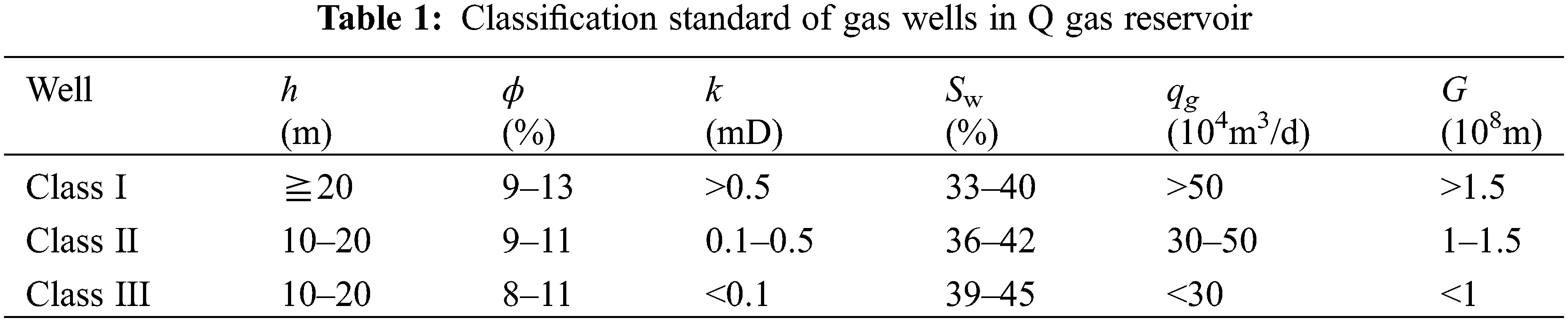
Considering the reservoir heterogeneity, the experimental core covered three types of wells (Classes I, II, and III), focusing on the main sand body of the main pay. A high-precision threshold pressure gradient test method—the capillary droplet movement monitoring method—was used to evaluate the threshold pressure gradient. Variable internal pressure and constant confining pressure under in situ conditions were mainly used to simulate stress sensitivity.
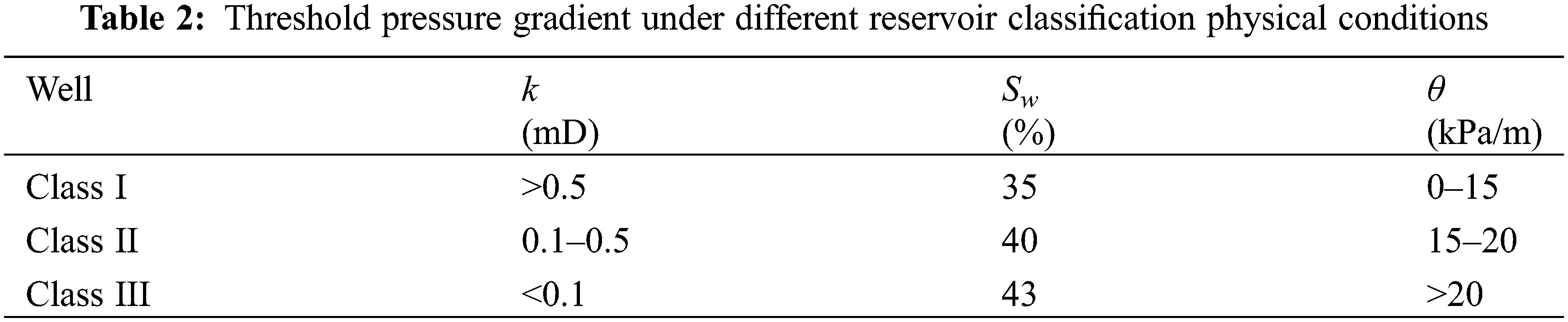
The relationship between water saturation and threshold pressure gradient under different porosity and permeability conditions has a semilogarithmic curve (Fig. 1). According to the classification of geological reservoirs, it was determined that the threshold pressure gradient of Class I wells was less than 15 kPa/m, whereas that of Class II wells was between 15 and 20 kPa/m, and that of Class III wells was greater than 20 kPa/m (Table 2).
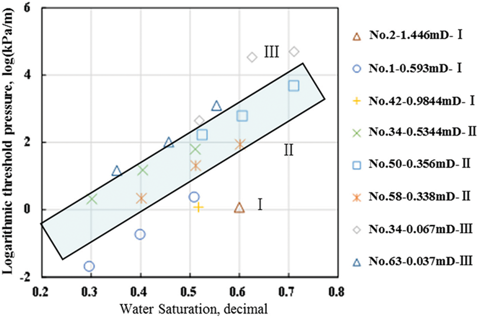
Figure 1: Semilogarithmic relationship between water saturation and threshold pressure gradient
The experimental results indicate that the lower the permeability of the Q gas field, the greater the stress sensitivity coefficient (SSC). The correlation between the SSC and permeability of Q gas reservoirs was obtained through regression. As shown in Fig. 2, the SSCs (α) of Classes I, II, and III wells were 0.002, 0.008, and 0.012 MPa−1, respectively.
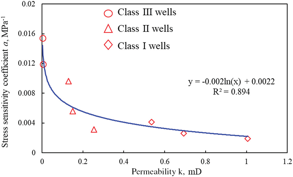
Figure 2: Relationship between the stress sensitivity coefficient and permeability of the Q gas reservoir
3 Numerical Simulation Considering the Special Seepage Mechanism
The relationship between the flow rate and pressure gradient is asymptotically linear in tight cores at a high-pressure gradient. At a low-pressure gradient, flow is impaired, and the flow rate is close to zero [25]. In a reservoir development process, the formation pressure drop causes rock skeleton deformation in the reservoir, whereas a change in the porosity and permeability of the reservoir decreases the flow capacity of fluid in it [26,27]. Therefore, the seepage model was established in consideration of the influence of the threshold pressure gradient and stress sensitivity. According to the nonlinear seepage model of threshold pressure gradient, the seepage curve was assumed to meet the following three criteria:
1) Strict monotonicity, i.e., as the pressure gradient increases, the velocity increases.
2) Slow start-up characteristic:
3) Asymptotic linearity:
Based on the hypothesis, the following nonlinear seepage model was given [25]:
The nonlinear seepage model obtained by deformation is as follows:
This can be written in vector form as follows:
When considering stress sensitivity, we have
In accordance with the given model, the nonlinear seepage mathematical equations can be established, solved, and simulated using numerical simulation software. The numerical simulation method considering the special seepage mechanism was based on the actual channel sand body shape, reservoir physical properties, gas reservoir temperature and pressure, fluid physical properties, and drilling and completion parameters. Through numerical simulation, the well spacing of different types of gas wells was further evaluated and compared with the result of the inverse dynamic reserve algorithm considering the special seepage mechanism.
In accordance with the geological characteristics of the Jurassic Shaximiao Formation gas reservoir in the Q gas field, the Implicit-Explicit (IMEX) module of CMG (a commercial simulator software) was used to establish the reservoir numerical model. The CMG software was used to simulate the underground migration and physical and chemical processes of oil, gas, and water under various complex geological conditions. The IMEX module is CMG’s new generation adaptive implicit-explicit black-oil and unconventional reservoir simulator, which includes various features, and was developed to simulate primary depletion and coning as well as water, gas, solvent, and polymer injection in single and double porosity reservoirs. Its grid is divided into I × J × K = 320 × 24 × 5, containing 38,400 grids, in which the value of each grid cell is 25 m × 25 m × 4 m. The established model is shown in Fig. 3.
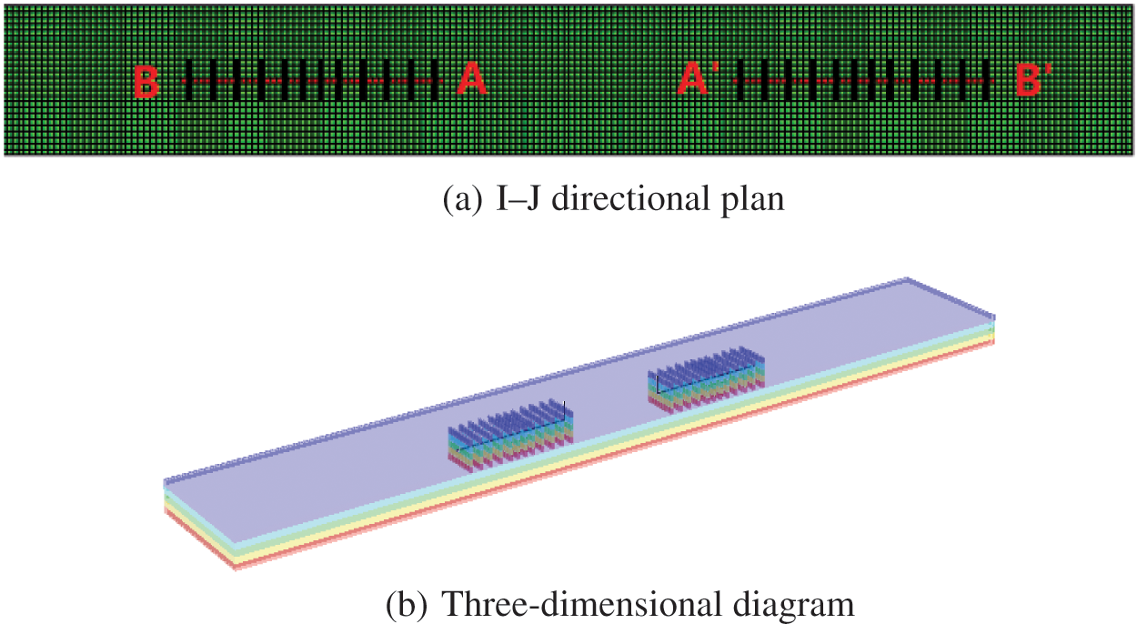
Figure 3: Numerical simulation model of fractured horizontal well
The permeability of the Jurassic Shaximiao Formation gas reservoir in the Q gas field ranged from 0.05 to 0.5 mD, the gas saturation ranged from 57% to 65%, the porosity ranged from 10% to 12%, the middle depth was 2,500 m, the effective thickness was in the range of 15–20 m, and the original formation pressure was 23 MPa. The basic parameters are shown in Table 3, and the phase permeability curve is shown in Fig. 4. The threshold pressure gradient was set by “PTHRESH(I J K) *MATRIX CON” in the module, and the SSC was set according to k = kie−α(pi-p) in the module to the corresponding permeability value when the pressure changed, where pi and ki denote the initial pressure and permeability, respectively, p and k denote the changing pressure and corresponding permeability, respectively, and α was the SSC.
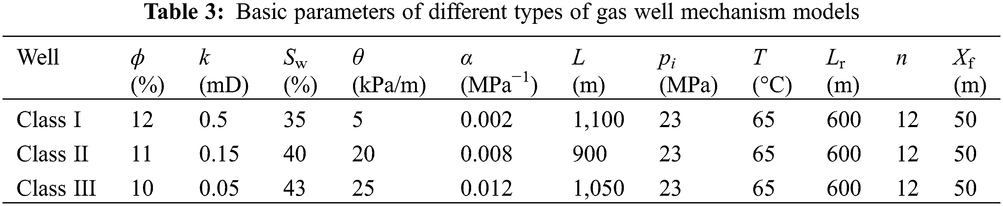
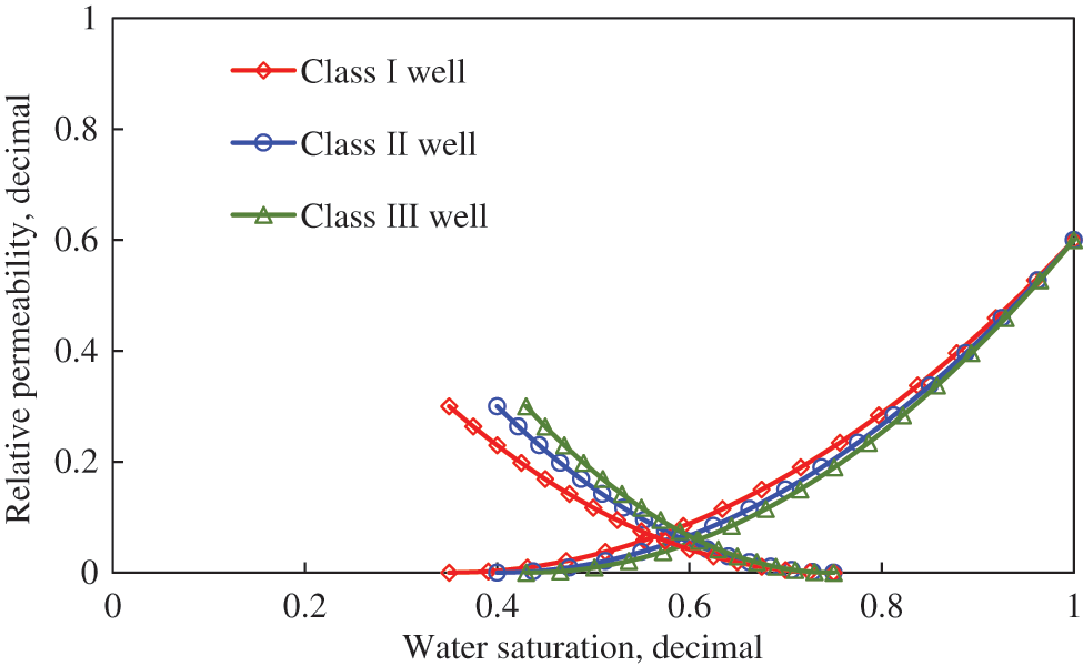
Figure 4: Relative permeability curves of different gas wells
According to the cumulative production curve in Fig. 5 and the formation pressure distribution diagram in Fig. 6, when well spacing for the primary development (distance of point AA’) of all well classes was less than 400 m, the inter-well interference was severe and impaired development. Therefore, increasing well spacing could improve the control and production of reserves as well as increase the cumulative production of well groups. However, too large well spacing could cause insufficient use of inter-well reserves and an insignificant increase in well group production. When the well spacing for the primary development of Class I wells reached 800 m, the growth in output of gas wells began to decline, and when it was greater than 1,000 m, the cumulative production did not increase significantly, and the reserves between wells with too large spacing were not fully utilized.
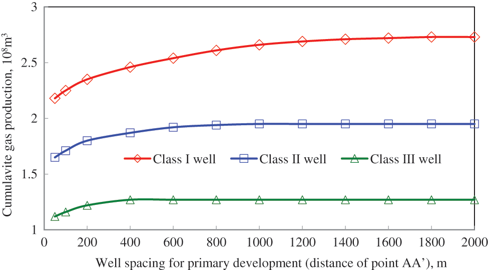
Figure 5: Cumulative production of different types of wells with different well spacing
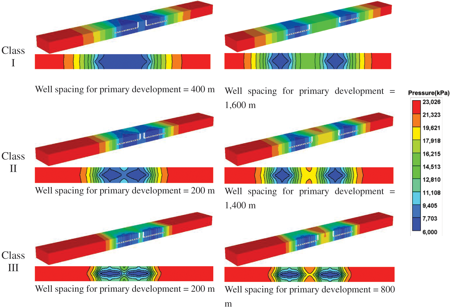
Figure 6: Formation pressure distribution of different types of wells with different well spacing (10 years of production)
When the well spacing for the primary development of Class II wells was less than 200 m, the interference between wells was severe and the cumulative gas production was low, when it reached 600 m, the increase in production declined, and when it was greater than 800 m, the cumulative gas production did not increase, as the greater the distance between wells, the less reserves were used.
For Class III wells, when the well spacing was less than 200 m, the production of gas wells was somewhat affected; and when it was greater than 400 m, the inter-well reserve utilization decreased, which affected the ultimate recovery efficiency.
Taking the midpoint of AA’ as a reference, we calculated the pressure derivatives. According to the pressure derivative vs. time data plotted in Figs. 7–9, when the well spacing in Class I wells reached 1,000 m, the pressure derivative curve gradually became less steep and the pressure change became smaller after a certain production period. When the well spacing in Class II wells was greater than 600 m and that in Class III wells reached 400 m, the pressure derivative curve gradually became stable after a certain production period and the pressure change became smaller.
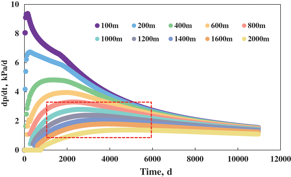
Figure 7: Pressure derivative of Class I wells with different well spacing
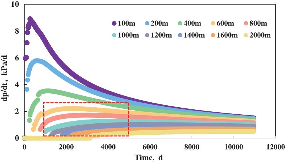
Figure 8: Pressure derivative of Class II wells with different well spacing
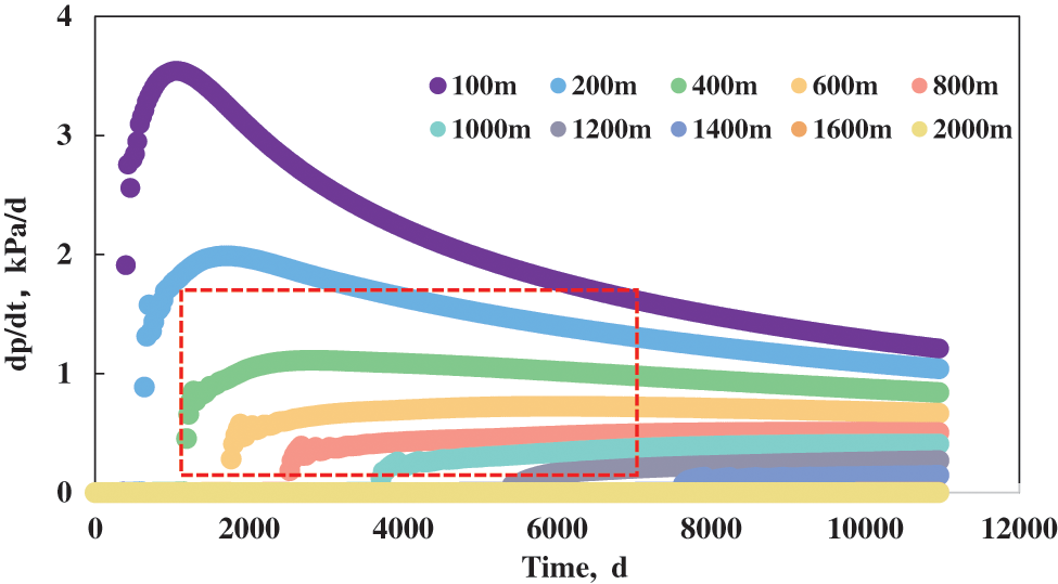
Figure 9: Pressure derivative of Class III wells with different well spacing
Based on the cumulative production curve, formation pressure distribution diagram, and pressure derivative curve, the well spacing for the primary development of Class I wells was 800–1,000 m, while that of Class II wells was 600–800 m, and that of Class III wells was 200–400 m.
4 Calculation of Well Spacing for Primary Development Based on the Inverse Dynamic Reserve Algorithm
Our numerical simulation model could determine the well spacing for the primary development of different types of gas wells. Consequently, when the geological parameters and production parameters were complete, the inverse dynamic reserve algorithm could determine the well spacing for primary development more reliably. Based on the dynamic reserve method, single-well dynamic reserves were estimated to obtain the effective seepage area of the gas well within the well control range. Combined with the distribution characteristics of the reservoir and channel width, the well drainage boundary was adjusted to obtain a method for determining the drainage range of the narrow channel reservoir (Fig. 10).
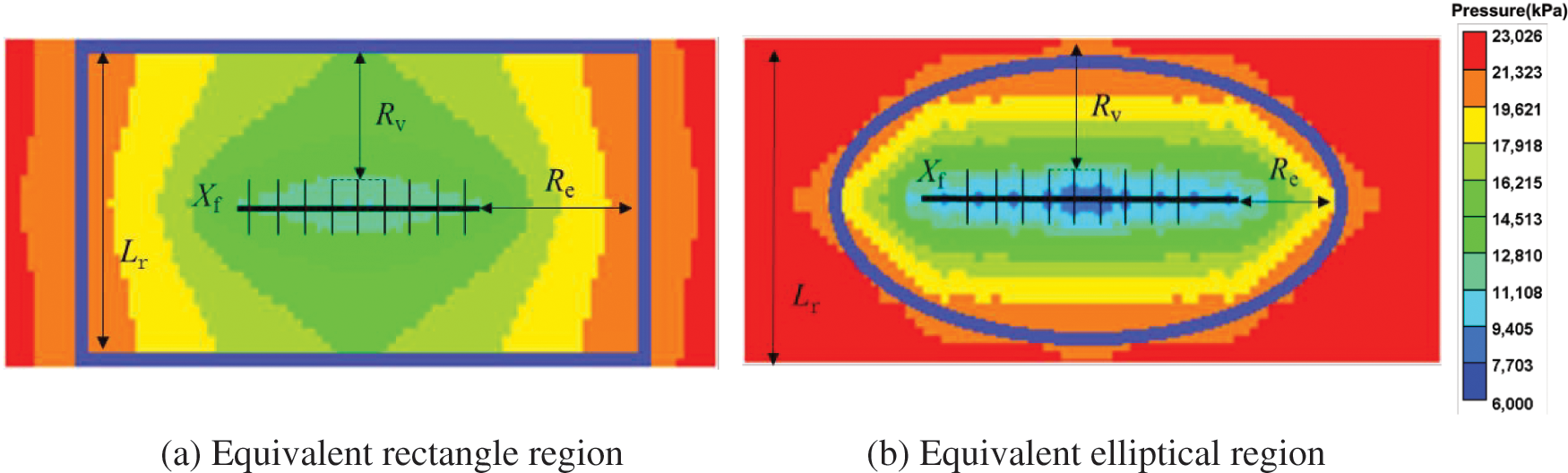
Figure 10: Equivalent diagram of different drainage areas
Combining the experimental results of threshold pressure gradient and stress sensitivity with the numerical simulation model of fractured horizontal wells showed that the pressure propagation of Classes I and II wells generally reached the boundary, i.e., 2(Rv + Xf) > Lr. According to the channel width and total area, the well spacing was equivalent to a rectangle.
Most of the pressure waves of Class III wells did not reach the boundary, i.e., 2(Rv + Xf) ≤ Lr, which can be represented by an equivalent elliptical region for the well spacing. The numerical simulation model of Class III wells was used to calculate the ratio of well distance and terminal extrapolation distance in the profile direction, Rv/Re. Several years of production were subsequently simulated. With a 10% drop in the initial reservoir pressure as a certain pressure change contour, Rv/Re was calculated from the pressure profile for each year and averaged (Fig. 11). We obtained Rv/Re = 1.12, which provided a basis for determining the effective seepage area of the gas well in the next step.
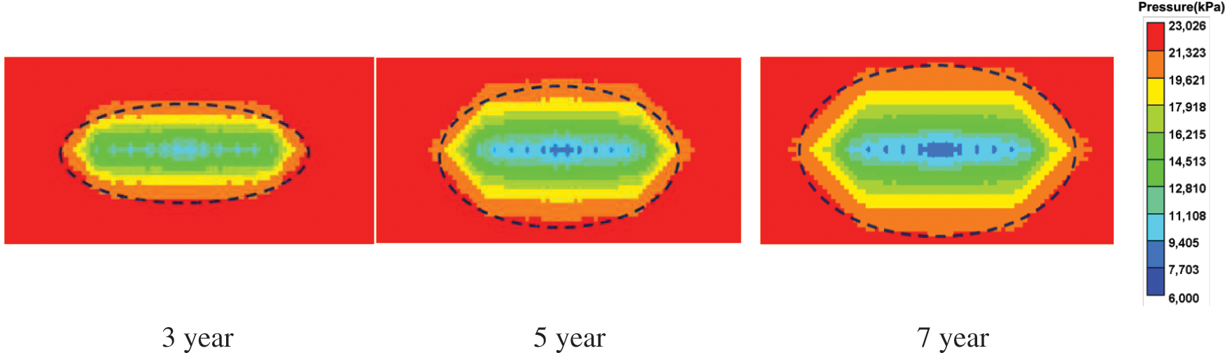
Figure 11: Drainage areas of Class III wells at different times
From the dynamic reserves of a single well, the reserve control area can be determined as follows:
where A denotes the reserve control area (m2), sgi denotes the original gas saturation, h denotes the reservoir thickness (m), ϕ denotes the porosity, G denotes the dynamic reserves (m3), Bgi denotes the volume factor (m3/sm3), and a is the coefficient.
The effective seepage area of a gas well can be determined according to the well control range (Figs. 12 and 13) as follows:
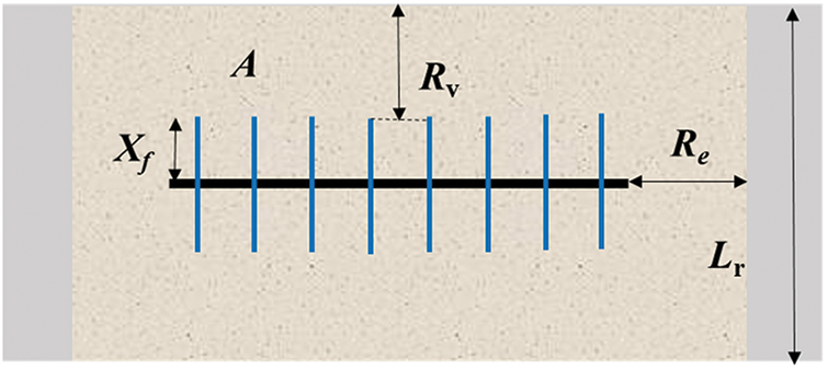
Figure 12: Equivalent rectangular diagram of the well control area
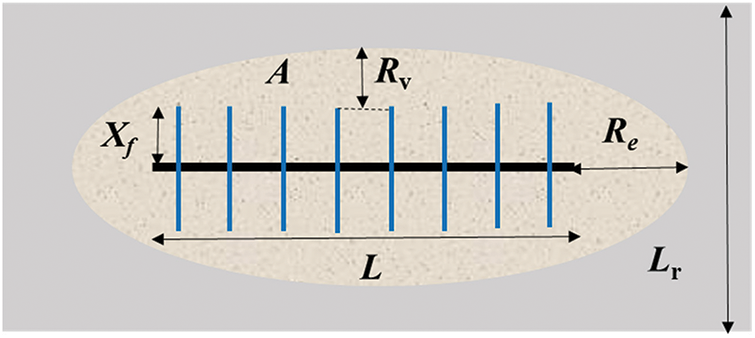
Figure 13: Equivalent elliptical diagram of the well control area
Rectangle:
Ellipse:
where L denotes the effective horizontal segment length (m), Xf denotes the fracture half-length (m), Re denotes the extrapolation distance (m), Rv denotes the radial extrapolation distance (m), and Lr denotes the channel width (m).
The well spacing Lp for the primary development can be calculated as follows:
Rectangle:
and
Ellipse:
The average dynamic reserves per well of Classes I, II, and III wells were 3 × 10⁸, 1.5 × 10⁸, and 0.579 × 10⁸ m3, respectively. Combined with the basic parameters of different types of wells in Table 3, well spacing of 802 and 662 m for Classes I and II wells, respectively, were obtained using Eq. (9), and a well spacing of 285 m for Class III wells was obtained using Eq. (10). The calculated results agree well with the numerical simulations. The numerical simulation is based on the actual geological and engineering parameters to establish a mechanism model that can determine the well spacing range for the primary development of different types of gas wells in the Q gas field. When a gas well has a certain production time and complete geological parameters, the inverse algorithm based on dynamic reserves can be used to estimate the well spacing. Combining the two methods, the well spacing ranges for the primary development of Classes I, II, and III wells were estimated to be 802–1,000, 600–662, and 285–400 m, respectively, with averages of 901, 631, and 342.5 m, respectively.
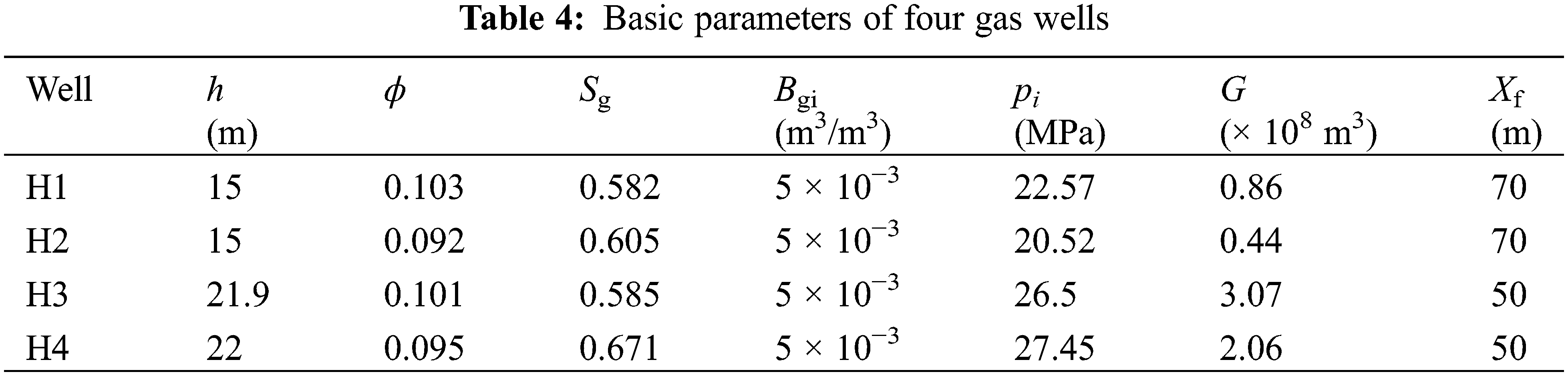
As shown in Fig. 14, H1 and H2 were two parallel fractured horizontal wells, that is, the line between the horizontal intervals and the center of the two wells was vertical, and the distance between the wells was 365–551 m. According to the classification of wells given in Table 1, H1 and H2 were Class III gas wells. As shown in Fig. 15, H3 and H4 were two series fractured horizontal wells, that is, the horizontal intervals of the two wells were linearly arranged, and the distance between point AA’ was about 529 m. Accordingly, H3 and H4 were classified as Class I wells. The basic parameters of the wells are presented in Table 4.
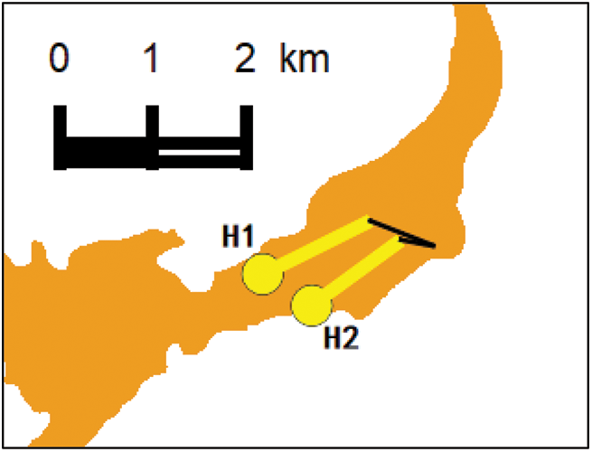
Figure 14: Geographical locations of wells H1 and H2
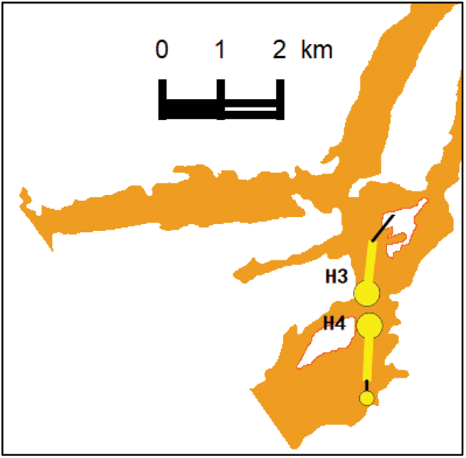
Figure 15: Geographical locations of wells H3 and H4
The pressure and gas production of wells H1 and H2 from March 21 to May 09, 2022 had relatively consistent characteristics, and the interference well test pressure of the two wells had basically the same static pressure as the formation, which may be in the same pressure system, as shown in Figs. 16 and 17. The abnormal fluctuation in the red circles in Fig. 17 indicates interference from the manometer.
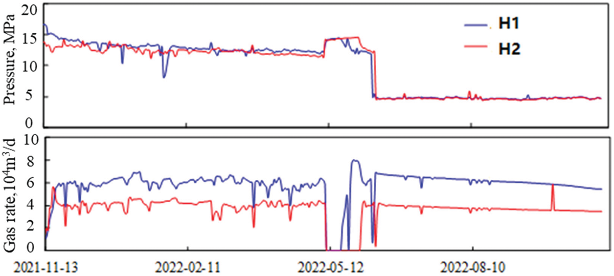
Figure 16: Production curve of H1 and H2
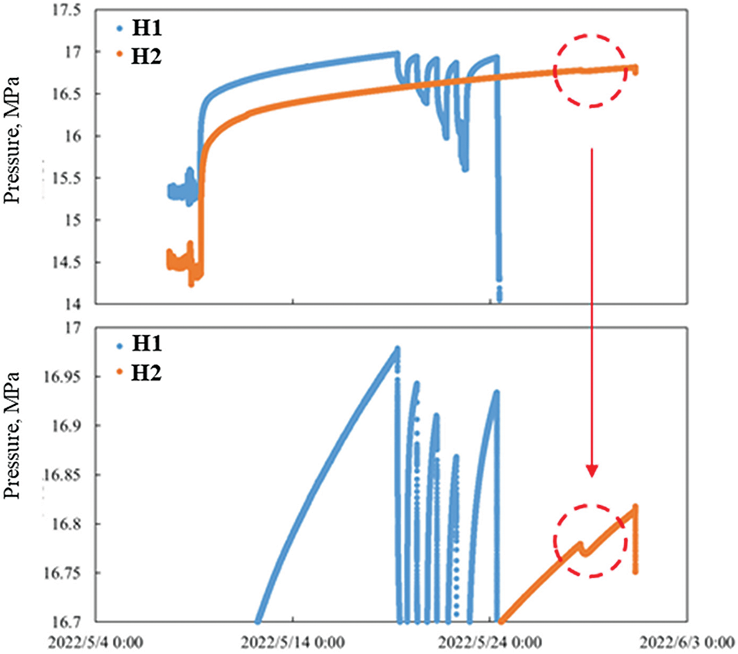
Figure 17: Manometer characteristics of interference test of H1 and H2
Well H2 was shut in for a long time, and the build-up curve of H2 dropped during the opening and production of H1. In accordance with Rv/Re = 1.12, the well spacing for the primary development of H1 and H2 was calculated to be 305 and 192 m, respectively, which was consistent with the numerical and analog results. Thus, it was calculated that the well spacing perpendicular to the horizontal intervals should be (305+192)/2 × 1.12 + 70 + 70 ≈ 418 m, which was greater than the nearest distance between the two wells by 365 m, indicating the existence of an interference effect, which was consistent with the actual situation.
Both H3 and H4 had reached the boundary flow stage due to their good physical properties and sufficient production time. However, the regularized production curve had a downward deviation in the Blasingame curve shown in Figs. 18 and 19, indicating that their productivity declined too fast in the later period and there was a possibility of interference effects. The calculated primary development well spacing of H3 and H4 was 719.6 and 706.16 m, respectively, which was greater than the actual point AA’ distance of the two wells by 529 m, indicating that there was reasonable inter-well interference between the two wells, which was consistent with the actual production situation.
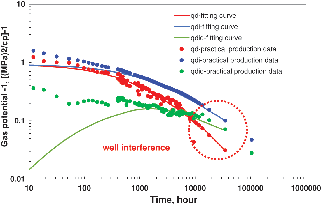
Figure 18: Blasingame curve of H3
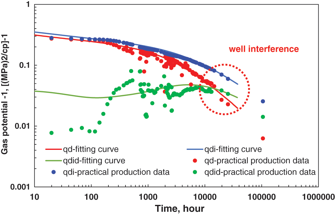
Figure 19: Blasingame curve of H4
Based on a numerical simulation model of well spacing for the primary development of fractured horizontal wells considering the special seepage mechanism and an inverse dynamic reserve algorithm with different equivalent drainage areas, the well spacing of fractured horizontal wells in tight gas reservoirs was evaluated, and the following conclusions were obtained:
1) According to the threshold pressure gradient and stress sensitivity test under different porosity and permeability conditions, it was determined that the threshold pressure gradient of Class I wells was less than 15 kPa/m, while that of Class II wells was between 15 and 20 kPa/m, and that of Class III wells was greater than 20 kPa/m, with SSCs of 0.002, 0.008, and 0.012 MPa−1, respectively.
2) The well spacing ranges for the primary development of Classes I, II, and III wells were 802–1,000, 600–662, and 285–400 m, respectively, with averages of 901, 631, and 342.5 m, respectively.
3) By considering both the pairs of parallel well groups and series well groups as examples, combined with the production dynamic characteristics and the analysis of interference effect, the calculation results of the well spacing for the primary development were verified to be reasonable and consistent with the actual production situation.
Acknowledgement: The authors are grateful to the reviewers whose constructive and detailed critique contributed to the quality of this paper.
Funding Statement: This study was financially supported by the Major Science and Technology Project of Southwest Oil and Gas Field Company (2022ZD01-02).
Author Contributions: The authors confirm contribution to the paper as follows: study conception and design: Fang Li, Haiyong Yi, Lihong Wu; data collection: Fang Li, Lingyun Du; analysis and interpretation of results: Fang Li, Juan Wu; draft manuscript preparation: Fang Li, Yuan Zeng. All authors reviewed the results and approved the final version of the manuscript.
Availability of Data and Materials: The datasets generated or analyzed during this study are available from the corresponding author on reasonable request.
Conflicts of Interest: The authors declare that they have no conflicts of interest to report regarding the present study.
References
1. Jia, C. Z. (2004). SEC oil and gas reserve evaluation method, pp. 2–27 (In Chinese). Beijing, China: Petroleum Industry Press. [Google Scholar]
2. Hu, Y. D., Xiao, D. M., Wang, Y. X. (2004). Basic principles of oil and gas proven reserves evaluation according to SEC standard. Acta Petrolei Sinica, (2), 19–24 (In Chinese). https://doi.org/10.3321/j.issn:0253-2697.2004.02.004 [Google Scholar] [CrossRef]
3. Etherington, J. R. (2009). Managing your business using integrated PRMS and SEC standards. SPE Annual Technical Conference and Exhibition, SPE-124938-MS. https://doi.org/10.2118/124938-MS [Google Scholar] [CrossRef]
4. Zainul, A. J., Rosly, M., Hong, T., Egbogah, E. O., Musbah, A. W. et al. (1997). An integrated approach to petroleum resources definitions, classification and reporting. SPE Asia Pacific Oil and Gas Conference and Exhibition, Kuala Lumpur, Malaysia. https://doi.org/10.2118/38044-MS [Google Scholar] [CrossRef]
5. SPE/WPC/AAPG/SPEE (2007). Petroleum resources management system. http://large.stanford.edu/courses/2013/ph240/zaydullin2/docs/prms.pdf (accessed on 28/02/2007). [Google Scholar]
6. SPE/WPC/AAPG/SPEE (2011). Guidelines for application of the petroleum resources management system. https://i2massociates.com/downloads/PRMS_Guidelines_Nov2011.pdf (accessed on 01/11/2011). [Google Scholar]
7. Harrell, D. R., Gardner, T. L. (2005). Significant differences in proved reserves estimates using SPE/WPC definitions compared to United States Securities and Exchange Commission definitions. SPE Reservoir Evaluation & Engineering, 8(6), 520–527. [Google Scholar]
8. Kang, A. (2010). Update and comparison of SPE and SEC oil & gas reserve evaluation specifications. International Business, 18(6), 61–64. https://doi.org/10.3969/j.issn.1004-7298.2010.06.012 [Google Scholar] [CrossRef]
9. Morales, E., Lee, W. J. (2020). SEC and PRMS proved reserves: Differences due to varying interpretations of final investment decision. SPE Europec Featured at 82nd EAGE Conference and Exhibition, SPE-200626-MS. Amsterdam, Netherlands. [Google Scholar]
10. Securities and Exchange Commission (2009). Modernization of oil and gas reporting. Federal Register, 74(9), 2158–2197. [Google Scholar]
11. Zhao, W. Z., Li, J. Z., Wang, Y. X., Bi, H. B. (2006). Methods of determining proved reserves by SEC standard. Petroleum Exploration and Development, 33(6), 754–758 (In Chinese). https://doi.org/10.3321/j.issn:1000-0747.2006.06.021 [Google Scholar] [CrossRef]
12. Zhang, L., Wei, P., Xiao, X. Z. (2011). Characteristics and influencing factors of SEC reserves evaluation. Oil & Gas Geology, 32(2), 293–301 (In Chinese). https://doi.org/10.1007/s12182-011-0123-3 [Google Scholar] [CrossRef]
13. Wang, S. H., Wei, P. (2012). Dynamic evaluation and analysis of SEC reserves. Petroleum Geology and Recovery Efficiency, 19(2), 93–94+117–118 (In Chinese). https://doi.org/10.3969/j.issn.1009-9603.2012.02.028 [Google Scholar] [CrossRef]
14. Lu, J., Liu, C. C., Liao, K. G., Ma, L. M., Liu, Y. et al. (2019). SEC reserves evaluation method of Changxing Formation gas reservoir in Yuanba gas field. Natural Gas Industry, 39(S1), 184–186 (In Chinese). [Google Scholar]
15. Feng, X. X., Liao, X. W. (2020). Study on well spacing optimization in a tight sandstone gas reservoir based on dynamic analysis. ACS Omega, 5(7), 3755–3762 [Google Scholar] [PubMed]
16. Chen, J. Y., Wei, Y. S., Wang, J. L., Wei, Y., Qi, Y. D. et al. (2021). Inter-well interference and well spacing optimization in shale gas reservoir. Journal of Natural Gas Geoscience, 6(5), 301–312. https://doi.org/10.11764/J.JNGGS.2021.09.001 [Google Scholar] [CrossRef]
17. Wang, S. P. (2021). Method for determining horizontal well drainage range in plane heterogeneous fluvial reservoir. Science Technology and Engineering, 21(16), 6677–6680 (In Chinese). https://doi.org/10.3969/j.issn.1671-1815.2021.16.021 [Google Scholar] [CrossRef]
18. Kang, S. S., Datta-Gupta, A., John Lee, W. (2013). Impact of natural fractures in drainage volume calculations and optimal well placement in tight gas reservoirs. Journal of Petroleum Science and Engineering, 109, 206–216. https://doi.org/10.1016/j.petrol.2013.08.024 [Google Scholar] [CrossRef]
19. Gelbunuv, A. T. (1987). Oil development of abnormal reservoirs. Beijing, China: Publication House of Petroleum Industry. [Google Scholar]
20. Feng, W. G. (1986). Current circumstance and development of researching in no-Darcy low speed percolation. Journal of Petroleum Exploration and Development, 13(4), 76–80. [Google Scholar]
21. Song, F. Q., Liu, C. Q., Li, F. H. (1999). Transient pressure of percolation through one dimension porous media with threshold pressure gradient. Applied Mathematics and Mechanics, 20(1), 27–35. [Google Scholar]
22. Prada, A., Civan, F. (1999). Modification of Darcy’s law for the threshold pressure gradient. Journal of Petroleum and Science Engineering, 22(4), 237–240. https://doi.org/10.1016/S0920-4105(98)00083-7 [Google Scholar] [CrossRef]
23. Ning, B., Xiang, Z. P., Liu, X. S., Li, Z. J., Chen, Z. H. et al. (2019). Production prediction method of horizontal wells in tight gas reservoirs considering threshold pressure gradient and stress sensitivity. Journal of Petroleum Science and Engineering, 187, 106750. https://doi.org/10.1016/j.petrol.2019.106750 [Google Scholar] [CrossRef]
24. Dong, X. Y., Yang, J. Y. (2023). Numerical simulation of a two-phase flow with low permeability and a start-up pressure gradient. Fluid Dynamics & Materials Processing, 19(1), 175–185. https://doi.org/10.32604/fdmp.2022.021345 [Google Scholar] [CrossRef]
25. Wang, Y. (2021). Experimental study on the nonlinear flow model in tight reservoirs and the corresponding applications in the numerical reservoir simulation software (In Chinese). China: University of Science and Technology of China. [Google Scholar]
26. Zhao, N., Wang, L., Sima, L. Q., Guo, YH., Zhang, H. et al. (2022). Understanding stress-sensitive behavior of pore structure in tight sandstone reservoirs under cyclic compression using mineral, morphology, and stress analyses. Journal of Petroleum Science and Engineering, 218, 110987. https://doi.org/10.1016/j.petrol.2022.110987 [Google Scholar] [CrossRef]
27. Li, X. P., Cao, L. N., Luo, C., Zhang, B., Zhang, J. Q. et al. (2017). Characteristics of transient production rate performance of horizontal well in fractured tight gas reservoirs with stress-sensitivity effect. Journal of Petroleum Science and Engineering, 158, 92–106. https://doi.org/10.1016/j.petrol.2017.08.041 [Google Scholar] [CrossRef]
Cite This Article
 Copyright © 2024 The Author(s). Published by Tech Science Press.
This work is licensed under a Creative Commons Attribution 4.0 International License , which permits unrestricted use, distribution, and reproduction in any medium, provided the original work is properly cited.
 Downloads
 Citation Tools