Influence of Rail Fastening System on the Aerodynamic Performance of Trains under Crosswind Conditions

1  Introduction

The complex turbulence generated by high-speed train operation has become a focal point in the study of high-speed train aerodynamics. Aerodynamics plays an indispensable role in either reducing aerodynamic drag or ensuring high-speed operation safety. Hence, precise numerical methods and simulations closely resembling real environments are of great importance to obtaining accurate results.

The wind generated by high-speed train movement, also known as slipstream, poses a significant threat to passengers and staff near tracks [1], making it imperative to delve into the mechanism and development process of slipstream. In response, the European Standards Committee has issued European regulations on the maximum slipstream velocity of trains [2–4]. By observing the flow field structure around high-speed trains, it has been found that the front pressure, train wake, air flow in the bogie and the development of body boundary layer jointly form the slipstream of high-speed trains [5]. Factors affecting the slipstream of high-speed trains include not only the shape and aspect ratio of locomotive but also surrounding infrastructure [6,7] and environmental conditions [8]. Wang et al. [9] systematically compared the wakes of two geometric configurations with and without rails analyzed the influence of rails on the slipstream characteristics of high-speed trains and revealed the potential mechanisms by which rails shape wake structure. Bell found that a pair of wake vortices fell off the rear of the car and gradually shifted toward the ground over time. Even small-sized rails can have a certain impact on the formation and development of train wakes [10]. Wang et al. [11] revealed the influence of bogies on train slipstream and wake by studying the flow structure, slip flow characteristics and aerodynamic characteristics of train models without bogies and with simplified bogies. Utilizing the sliding mesh method and considering the shape of sleepers, Paz et al. [12] found that the drag coefficient of rains increased by 15% and the presence of sleepers facilitated ballast projection. Wang et al. [13] investigated the performance of three widely used models, namely Unsteady Reynolds-Average Navier-Stokes (URANS), Scale-Adaptive Simulation (SAS), and Detached Eddy Simulation (DES), in predicting the slipstream of full-scale train models, with an attempt to determine whether different turbulence modeling methods were suitable for simulating various aspects of slipstream. Some scholars also conducted field experiments on train slipstream. Soper et al. [14] measured the undercar flow characteristics and track properties of high-speed trains on a railway in southern England. Their research results revealed that on a well-performing track, the mechanical and aerodynamic forces associated with track displacement are of similar magnitude and track vibration had a greater impact on ballast motion for tracks with high acceleration and poor maintenance. Tschepe et al. [15] presented a comprehensive experimental and numerical study of boundary layer and skin friction along trains, focusing on Reynolds number effects. Methods for transferring drag measurements from reduced-scale train models to corresponding full-scale vehicles are presented. Rochard et al. [16] address a well-known tool for calculating the resistance to train motion and its applicability in describing high-speed operation, which also allows for the estimation of the contribution of various features of the train structure to aerodynamic drag.

Crosswind conditions are a common operational environment for trains. The presence of crosswinds introduces a yaw angle to the train, significantly deteriorating its aerodynamic performance and increasing energy consumption. Excessive crosswinds possibly lead to unstable train operation and even derailment. For safety reasons, trains typically reduce speed or come to a halt when faced with strong wind. A number of wind tunnel experiments [17–19] and numerical simulations have been conducted. It has been observed that under crosswind conditions, moving and stationary models exhibit certain differences in the aerodynamic performance of the train: The stationary model has approximately 5% lower lateral force and rolling moment coefficients, with a difference of about 12% from moving models in vertical force coefficient [20]. The aerodynamic characteristics of freight trains based on large eddy simulation models under crosswind conditions at a yaw angle of 90° have been studied. It has been discovered that airflow separates at the sharp leading edge of the container, forming a large, separated flow region on the top of the container [21]. The aerodynamic performance of high-speed trains under severe rain and strong crosswind conditions has also been thoroughly investigated using the Eulerian two-phase model, which will provide reference for the safe operation of trains under heavy rain and crosswind conditions [22]. Krajnović et al. [23] compared the large eddy simulation of the flow around the static model and the moving model with that of the simplified train model under crosswind conditions and found that several aerodynamic coefficients of the moving model recoil with those of the stationary model. The yawing moment coefficient displayed an overshoot of some 30%, which shows the importance of dynamic testing to meet safety standards. Giappino et al. [24] compared the crosswind behavior on a high-speed train with that on a low-speed train through two subsequent analyses, namely, measuring aerodynamic coefficients through wind tunnel tests on scale models and evaluating rollover risk by using Characteristic Wind Curve definition based on static equilibrium.

Traditional methods, such as wind tunnel test, assume trains to be stationary and set a fixed velocity-inlet while simulating wind blowing on the train, which deviates from real-world scenarios to some extent. However, the use of sliding mesh can effectively bridge this gap, better simulating the interaction between moving train, airflow, and ground facilities during operation. Niu et al. [25] analyzed and compared the aerodynamics of stationary and moving trains, as well as the flow field beneath the trains, finding that train motion significantly influences the distribution pattern and magnitude of the velocity field beneath the train. Sliding mesh technology has been widely employed in research areas such as trains passing through tunnels [26] and train-to-train interactions [27,28] because of its capability to better capture the flow field structure beneath trains and the slipstream of trains. In keeping with wind tunnel experiments [17–19], the study of aerodynamic characteristics of trains under crosswinds [20–24] is also increasing as a popular research field.

Most modern high-speed trains run on ballastless tracks, which are secured to a reinforced concrete floor by a fastening system. The fastening system is complex in structure, with numerous and densely distributed components. However, there is still a lack of in-depth research on its effect on the aerodynamic performance, slipstream, and wake of high-speed trains.

Existing studies on the aerodynamic characteristics of high-speed trains only establishes simple track structure but fail to consider the effect of fastening system. For example, Wang et al. [29] explored the effect of train height on the aerodynamic performance through the Improved Delayed Detached Eddy Simulation (IDDES) method. Reyes et al. [30] constructed a simple I-beam track for studying the effect of different aerodynamic configurations on the crosswind stability of conventional trains. Huo et al. [31] only modelled a simple track in the study of the effect of freight train formation on aerodynamic performance, and Sun et al. [32] did not even model a track in their study of slipstream improvement. Guo et al. [33] failed to account for the effect of tracks while investigating the aerodynamic characteristics of a two-car train. Luo et al. [34] discussed the safety of high-speed trains entering tunnels under crosswind conditions but ignored the effect of track modelling. In addition, some studies involving the characteristics of the flow field at the bottom of train, such as aerodynamic noise and snow accumulation in the bogie region, require the bottom flow field to be as close as possible to the actual scenario. However, track or fastener models are also easily overlooked in most studies. Shi et al. [35] only developed a simple track model when studying the aerodynamic noise characteristics in the bogie region. Snow icing in the bogie region has been a popular research issue in recent years, but most of the studies only established simple track models [36–38].

Therefore, there is an urgent need to study the effects of track as well as fastener models on the aerodynamic performance of trains, including bogie flow field, slipstream and wake vortex, to provide some references for high-speed train modelling in other fields. To this end, based on a three-car model of a high-speed train, this paper constructs a trackless ground model (NR), a trackless ground model (WR) and a track-fastening system ground model (WRFS) using sliding grid technology, and then evaluates the effects of rail and rail fastening systems on the aerodynamic force, slipstream velocity, and train wake under crosswind conditions using the IDDES method based on the SST k-ω turbulent model.

Firstly, geometry models, grid strategy and numerical methods are introduced and validated. Secondly, the aerodynamics of trains, slipstream assessment, and wake flow characteristics are compared and analyzed. Finally, the whole study is summarized.

2  Numerical Simulation Setup

2.1 Train Model

The CRH380B high-speed train is modelled at a ratio of 1:8, as shown in Fig. 1. The train consists of a front, middle and rear car. A more complete bogie system is adopted as this paper mainly focuses on the primary flow characteristics beneath the train. The geometric dimension is H (height of the train) = 0.486 m, W = 0.84 H and L = 19.7 H. The train is symmetric about the origin in the X and Y directions. Some of the smaller or not so significant structures of the train were simplified, such as intercar gaps, pantographs and air conditioning.

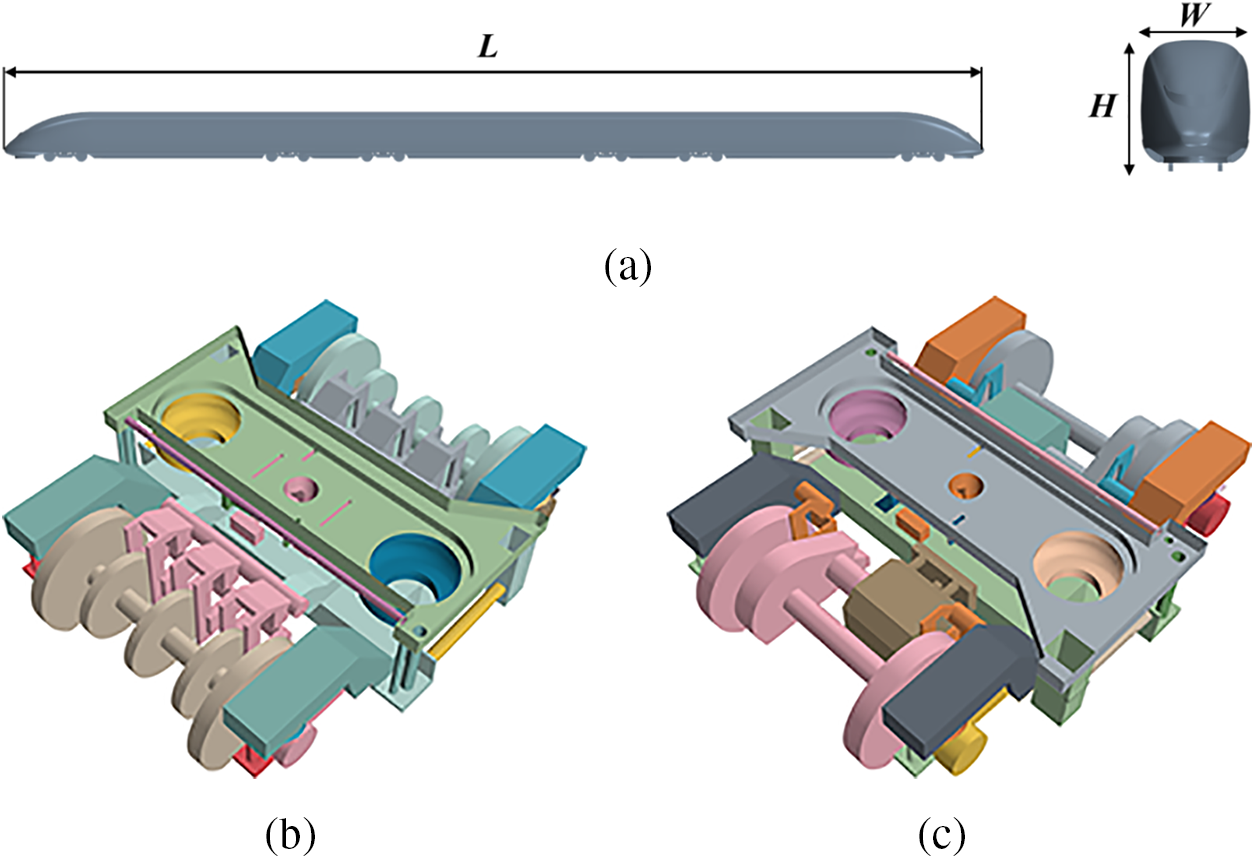
Figure 1: (a) Train model, (b) trailing bogie and (c) motor bogie

2.2 Rail Fastening System

The rail fastening system model adopted in this study is based on the Type 300 fastener, which can effectively adjust the rail height by adding shims, as shown in Fig. 2. The spacing between adjacent fasteners in the 1:1 scale model is 0.65 m. Fig. 3a–c respectively represents the NR, WR, and WRFS models.

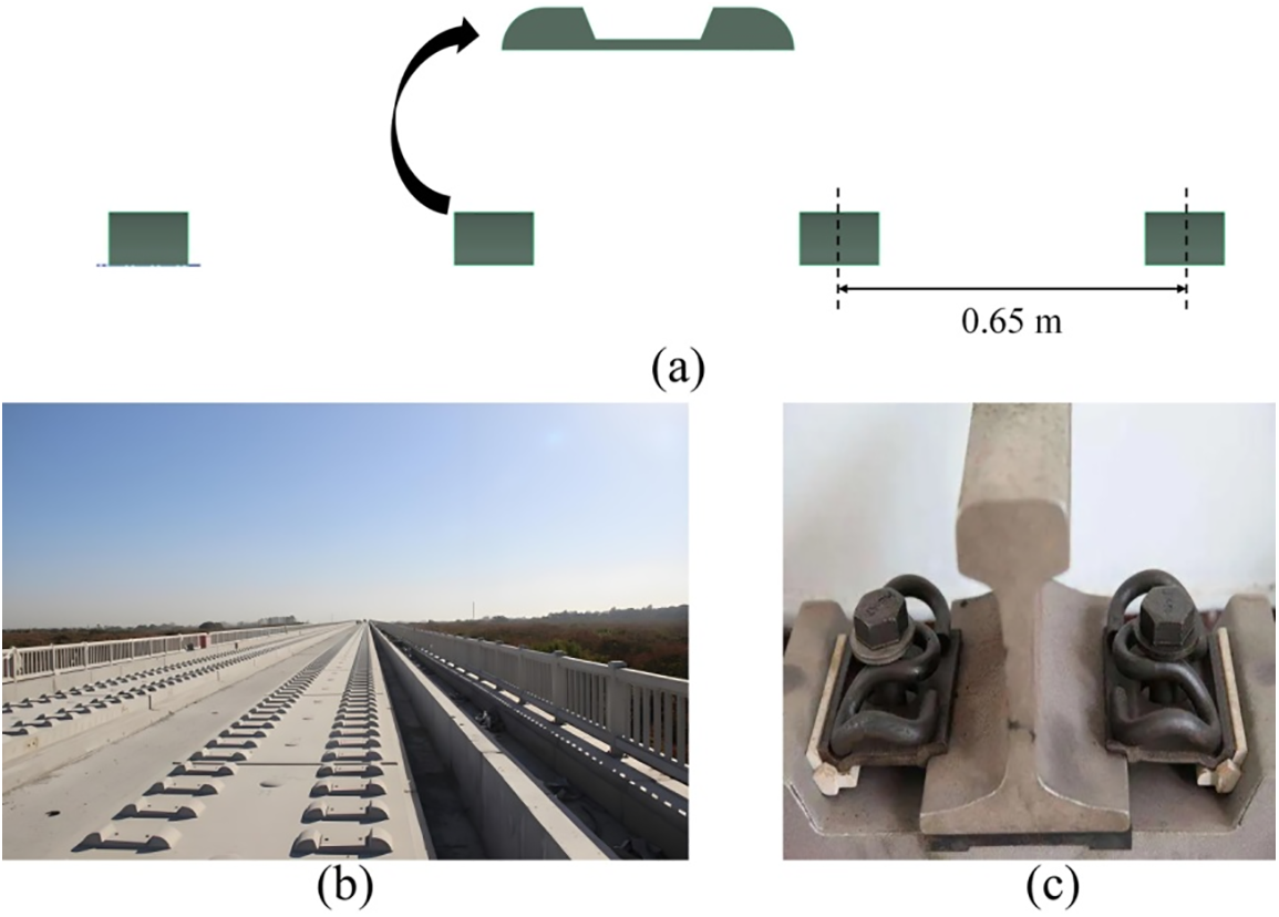
Figure 2: Rail fastening system: (a) positioning distance, (b) fastening system for a railway in Henan Province, China, and (c) connection of rails to fasteners

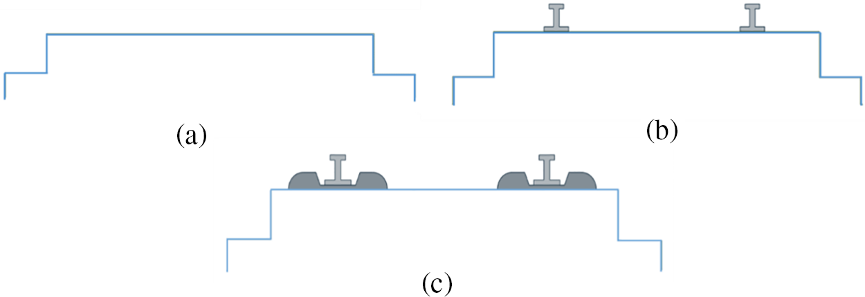
Figure 3: Computational cases: (a) NR, (b) WR and (c) WRFS

2.3 Computational Information

The same computational domain model is adopted for all the models and sliding mesh technology is utilized. The computational domain is divided into a stationary zone containing the ballastless track and a moving zone containing the train, as shown in Fig. 4. The inlet is 51.5 H from the nose of the train, and the outlet of the stationary zone is 15.4 H from the back of the train. The inlet of the stationary zone and the moving zone are on the same plane, and the length of the non-overlapping part of the two zones is 43.8 H m. The moving zone is 2.06 H high, and the stationary zone is 30 H wide and 11.6 H high. All the inlets and outlets of the computational domain are set as pressure outlets, with the ground and track as stationary walls, and the overlapping area of the stationary and moving zones as the interface. One side is set as a velocity inlet, and the other as a pressure outlet. The train speed is set to 250 km/h, meaning the moving zone advances at 69.44 m/s in the X-direction. The crosswind speed is set to 15 m/s in the Y-direction in accordance with the Regulations of the People’s Republic of China on the Technical Management of Railways (High-speed Railway Section). When crosswind speed is not greater than 15 m/s, the train can run at normal speed. Therefore, the maximum crosswind speed that the train can withstand when travelling at any permitted speed should be 15 m/s, which can be used as a typical wind speed for the present study.

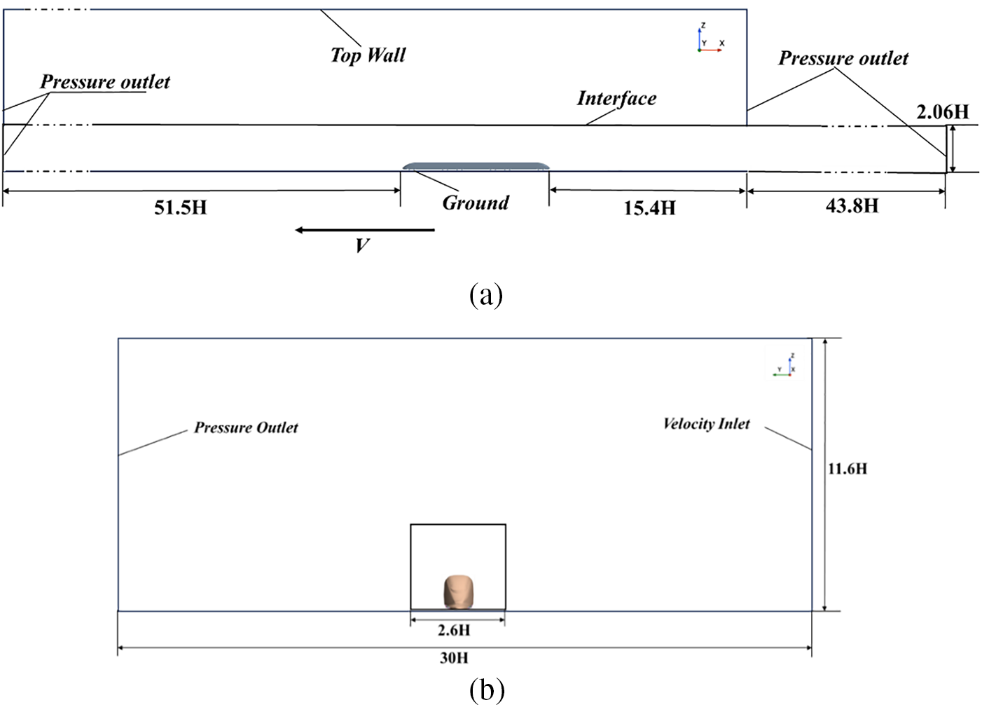
Figure 4: Computational domain: (a) side view and (b) front view

2.4 Numerical Method

ANSYS Fluent was used to solve the flow field in this paper. The Improved Delayed Detached Eddy Simulation (IDDES) method is employed in this paper because of its ability to achieve a balance between the low computational cost of the Reynolds-Averaged Navier-Stokes equation (RANS) and the high accuracy of Large Eddy Simulation (LES) method. In order to address the issues of grid dependency and high computational cost in LES simulations while overcoming the limitations of RANS simulations in accurately predicting turbulent structures, the IDDES method employs different turbulence models in the flow field. The RANS model is used for regions near the wall because of relatively small because turbulence scales in these regions, allowing the RANS model to more accurately capture turbulent effects. For regions far from the wall, However, the LES model is adopted for regions far from the wall due to larger turbulence structures in these regions, making the LES model more suitable for simulation. The above two models are switched typically based on the length scale of local turbulent structures. To be more specific, when this scale is below a certain value, the RANS model is utilized; when the scale is above a certain value, the LES model is employed. The length scale of the IDDES  lhyb is given by:

lhyb=f~d(1+fe)lRANS+(1−f~d)lLES (1)

where lRANS and lLES are the length scales of the RANS and LES models, respectively, fe=max{(fe1−1),0}Ψfe2 is the elevating function of the IDDES method, and

α=0.25−dΔ (2)

fB=min[2exp(−9α2),1] (3)

fe1={2exp(−11.09α2)ifα≥02exp(−9.0α2)ifα < 0 (4)

fe2=1−max(ftfl) (5)

where fe1 determines whether elevation has occurred, fe2 controls elevating intensity, d is the distance to the wall.

ft=tanh[(Ct2rdt)3] (6)

fl=tanh⁡[(cl2rdl)10] (7)

This paper employs a segregated solver based on the incompressible Navier-Stokes equation. The Semi-Implicit Method for Pressure Linked Equations Consistent (SIMPLEC) algorithm is used for pressure-velocity coupling. Turbulence terms are discretized using a second-order upwind scheme, while a hybrid scheme switching between bounded central differencing and second-order upwind schemes is used for convective term discretization. Second-order implicit time stepping is used for unsteady simulations. The time step is set to 0.00005 s to ensure temporal accuracy and numerical stability. The total simulation time is 0.325 s.

2.5 Grid Strategy

To capture finer flow field structures, grid refinement regions are respectively placed around the train, near the bogie and the rail fastening system. The dimensions of the bogie components, body surface, track mesh, two refinement zones around the body, and the refinement zones around the bogies are 2.5, 8, 1.25, 20, 10 and 5 mm, respectively, as shown in Fig. 4. The total thickness of the 15 boundary layers is 0.71 mm with a growth rate of 1.2. The value of y+ is basically around 1, which fits the range of k-ω turbulence model. Fig. 5 illustrates the details of the grid.

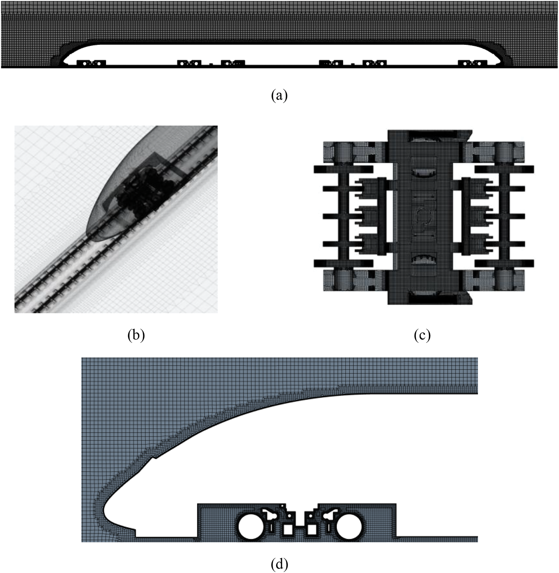
Figure 5: Computational grid: (a) refinement boxes, (b) surface mesh of train body, (c) surface mesh of bogie and (d) zoomed presentation of the mesh around the head

To eliminate the influence of grid number and quality on the calculation results, three sets of grids were generated for the CRH380B train. All refinement regions are the same. Fig. 6 shows the pressure coefficient along the centerline of the train surface under different numbers of grids. The pressure coefficients of fine and medium grids match very well at the front and rear of the train, indicating that there is a certain deviation between coarse and fine grids. Grid sensitivity tests demonstrate that the medium grid is sufficient for calculations. Based on the above settings, NR, WR, and WRFS respectively have 44.6 million, 48.62 million, and 65.88 million grids.

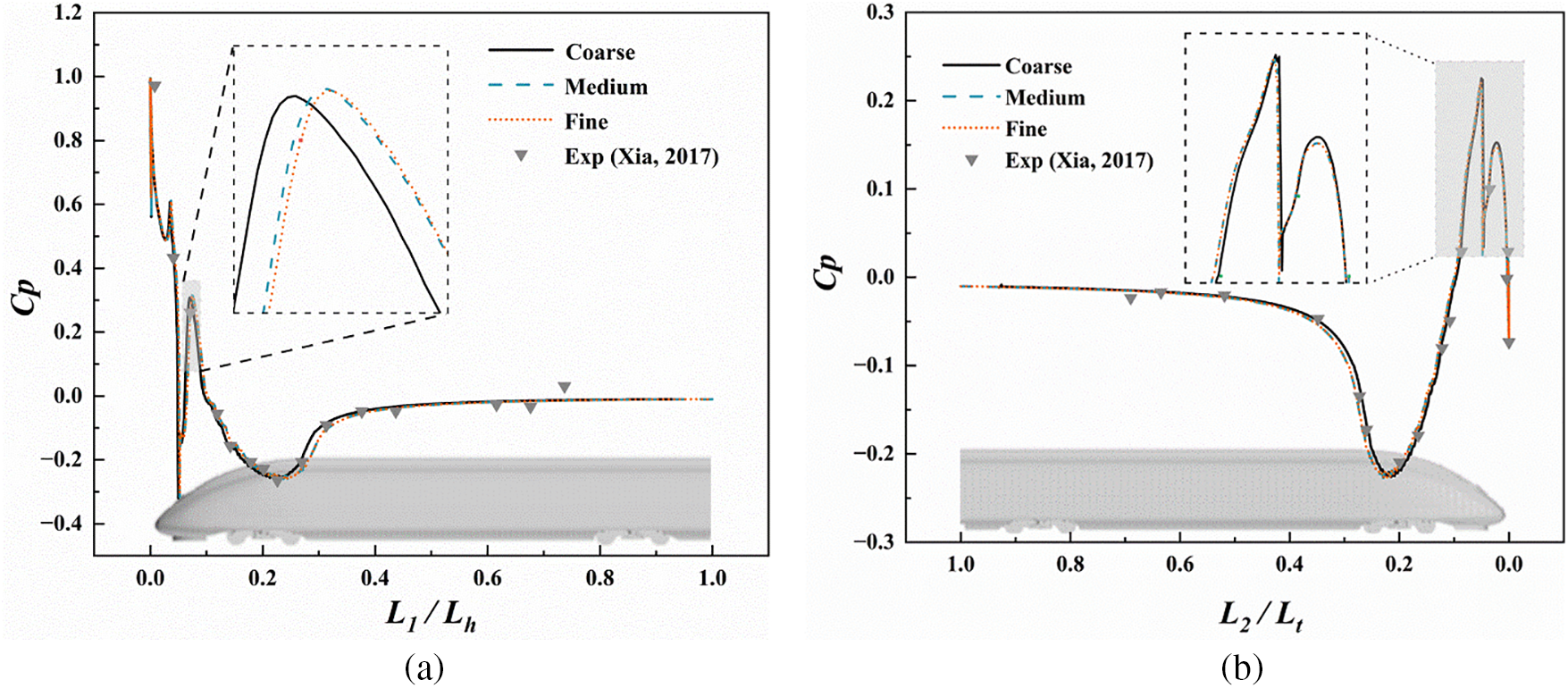
Figure 6: Comparison of pressure coefficient (Cp) for coarse, medium, fine zones and experimental results: (a) front car and (b) rear car (L1: distance to the head of the train, Lh: length of the head car; L2: distance to the tail of the train, LH: overall length of the tail car) [39]

2.6 Numerical Method Validation

2.6.1 Pressure Coefficient Validation

The IDDES method mentioned above was used to simulate the train running at a speed of 250 km/h without crosswind. The pressure coefficient of the train centerline (Cp) was extracted and compared with that obtained from the wind tunnel test conducted in the Shanghai Automotive Wind Tunnel [39], as displayed in Fig. 6. It can be clearly seen from the figure that there is good consistency between the two.

Cp=P−P∞0.5ρutrain2 (8)

where Cp is dimensionless pressure coefficient, P is surface pressure, P∞ is reference pressure, ρ is air density, and Utrain is the running speed of the train.

2.6.2 Train Slipstream Validation

The accuracy of numerical methods in predicting turbulent flow at the bottom of the train was verified by CFD and wind tunnel test. Slipstream velocity refers to the combined value of the streamwise velocity and the spanwise velocity. Vertical velocity is not considered because it does not pose a potential hazard to standing individuals. Slipstream velocity is made dimensionless by the following formula. The European Railway Agency has proposed two typical slipstream measurement locations, one of which is located 3 m from the center of the track and 0.2 m from the track surface while the other is located 3 m from the center of the track and 1.58 m from the track surface, which is equivalent to the height of railway platform. The former measurement location was selected and the distance was scaled accordingly by a factor of 1:8 in this study. The simulated slipstream velocity was compared with experimental data [40], as shown in Fig. 7.

Uslipstream=ux2+uy2utrain (9)

where Uslipstream is slipstream velocity, ux is streamwise velocity, uy is spanwise velocity, and Utrain is the running speed of the train.

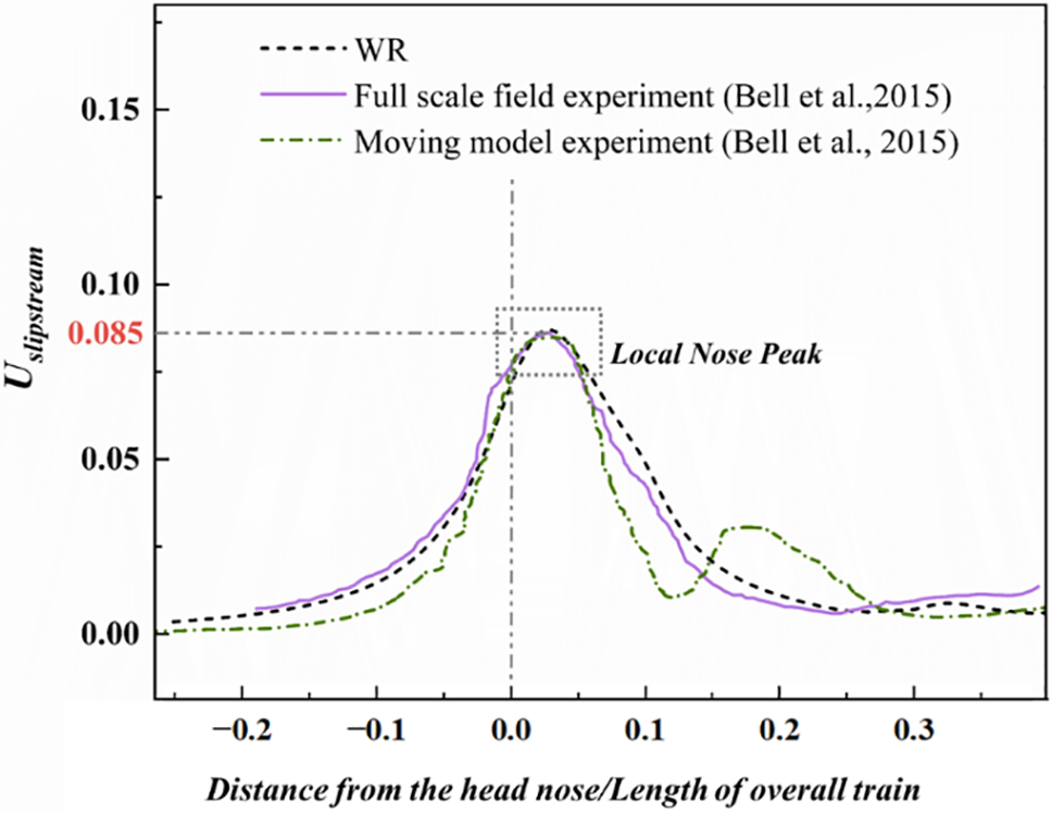
Figure 7: Validation of slipstream velocity at the monitoring position [40]

As shown in Fig. 7, the results obtained in this paper exhibit a similar trend to the experimental results. The sliding mesh technology used in this paper can effectively capture the slipstream peak at the front of the train, with a deviation of 1.86% compared to the moving model experiment and 2.32% compared to the full-scale model experiment. The agreement between the simulation and experimental results indicates that the numerical method used in this paper can accurately predict the slipstream velocity around the train.

3  Results and Discussion

This section is divided into three subsections. Section 3.1 compare the aerodynamic force performance of the train in three cases. Section 3.2 introduces the slipstream conditions of the train. Section 3.3 evaluates the wake of the train. To better compare the flow field changes caused by the slipstream around the train, some monitoring points were set up in front of the train in advance to monitor several physical quantities for subsequent analysis, as shown in Fig. 8. The monitoring points were sequentially named as p1–p13. After the calculation, the results obtained in the time domain were converted to the space domain, which was equivalent to obtaining the flow field from the front of the train to 7 m behind the tail of the train. In addition, to better analyze the flow field characteristics and wake of the train, several cross-sections were cut in the X- and Z-directions, as shown in Fig. 9.

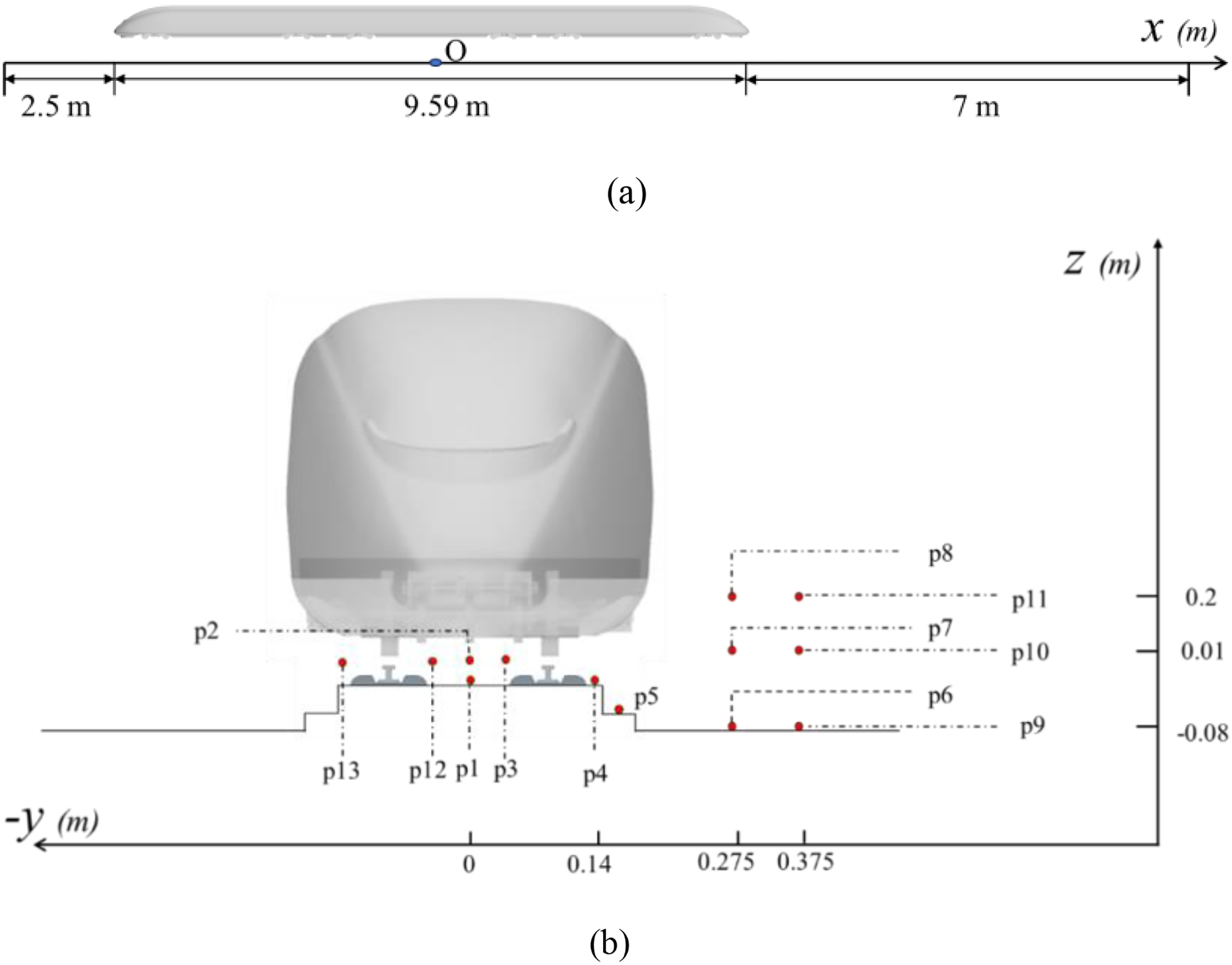
Figure 8: Schematic diagram of monitoring points: (a) range of monitoring distances, (b) specific location of monitoring points in the plane

Figure 9: Schematic diagram of cross-section: (a) x-section (b) z-section

3.1 Aerodynamic Force Analysis

Table 1 compares the drag force coefficients of front, middle and rear cars under different rail modeling methods. The drag force coefficient and lateral force coefficient of the train are converted by the following formulas. Obviously, the total drag force coefficients of the three track models under crosswind conditions are 0.4781, 0.4700, and 0.4700, respectively. The total drag force coefficients of WR and WRFS are the same, both of which are 1.69% lower than that of the NR model. Fig. 10 vividly illustrates the changes in drag force coefficients and lateral force coefficients of different parts of the train under different models. As shown in Fig. 10a, from NR to WR to WRFS, the drag coefficient of the front car slightly increases, while the drag force coefficient of the rear car gradually decreases. The drag force coefficient of the middle car is the largest for NR but the smallest for WR. The gradual decrease in the total drag force of the train is potentially caused by the changes in the flow around the train after the application of crosswind, which, combined with different track models, alters the forces on different parts of the train. Due to the streamlined design of the front of the train, most of the oncoming airflow is separated here. Moreover, it is obvious that the positive pressure on the front of the train is directed to the left and right sides, which will influence reducing the drag on the front of the train. This effect of distributing the pressure to both sides is not found in the middle and tail cars, so the resistance of the head car is less than that of the middle car. It can be learnt from the research of previous scholars that when the train is travelling at a certain speed, with the increase of crosswind speed, the resistance of the head car will gradually decrease, and the resistance of the middle and tail cars will gradually increase.

Cd=Fd0.5ρAutrain2 (10)

Cs=Fs0.5ρAutrain2 (11)

where Cd is dimensionless drag force coefficient, Cs is dimensionless lateral force coefficient, Fd  is drag force, Fs  is lateral force,  A is the positive projected area of the train in the X-direction, ρ is air density, and Utrain is the running speed of the train.

Figure 10: Comparison of drag and lateral force coefficients of different parts of the train (a) drag force coeffcient (b) lateral force coeffcient

Table 2 and Fig. 10b compare the lateral force coefficients of front, middle and rear cars, which are 1.3397, 1.3590, and 1.3513, respectively. They have the same pattern as that of the entire train, which is in the order of WR > WRFS > NR. Combined with Fig. 11, the reasons for such changes were also analyzed. Fig. 11 shows the pressure distribution at three sections of the tail of the train. It is evident from plane-x1 that there is a negative pressure center on the lee side of the train. The negative pressure area of WR and WRFS is larger than that of NR. Moreover, the negative pressure areas of WR and WRFS are closer to the train than that of NR, thus making the lateral forces of WR and WRFS greater than that of NR. The fundamental reason for the negative pressure areas to be close to the train body lies in the track structure. The track in the X-direction acts as a barrier to lateral flow, altering the direction of airflow, thus reducing the airflow passing under the bottom of the train and resulting in the leftward movement of the negative pressure center. For WRFS, the fastening system has many gaps, allowing more airflow to pass through and resulting in slightly smaller lateral force than WR.

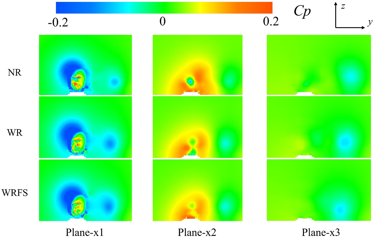
Figure 11: Comparison of pressure contours at three sections at the rear of the train

To investigate the differences in oscillation frequencies caused by track models, the power spectral density of the variations in drag force coefficient and lateral force coefficient was compared, as illustrated in Fig. 12. The results show that the power spectral density of different track models is basically consistent. Obviously, drag force coefficient and lateral force coefficient mainly oscillate in the low-frequency range, corresponding to f = 20–300 Hz, with a slight difference in the oscillation magnitude of their PSD at low frequency. In addition, new peaks in the PSD do not emerge after the track models are established, potentially due to its very small dimension of the track models and their limited influence on the forces acting on the train. Therefore, the oscillation frequency and dominant frequency of drag force coefficient and lateral force coefficient do not significantly change after the establishment of the track models.

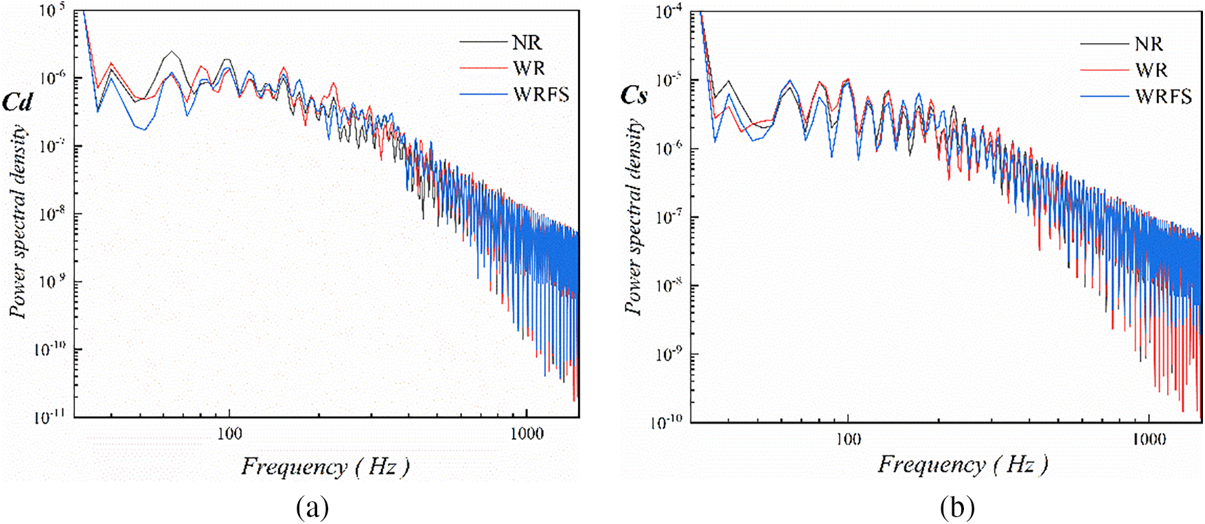
Figure 12: Comparison of power spectral density: (a) drag force coefficient (b) lateral force coefficient

Figs. 13 and 14 compare the time-average pressure distribution contour in the front, tail, and bottom of the train under crosswind conditions. As shown in Fig. 13, the time-average pressure coefficient distribution contours in the front of the train under the three models are basically identical. However, above the side cowcatcher at the rear of the train, a small negative pressure area emerges for WR and WRFS. As highlighted by red boxes in Fig. 14, there are differences in the time-averaged pressure coefficient distribution contour of the three among the bottom of the train cowcatcher, behind the first and third bogies, and at the front end of the rear cowcatcher. However, WR and WRFS are basically consistent, with some differences from NR. A reasonable explanation is that the track model, being close to the bottom of the train, alters the flow around the bottom of the train, resulting in changes in the pressure coefficient distribution contour of the train body.

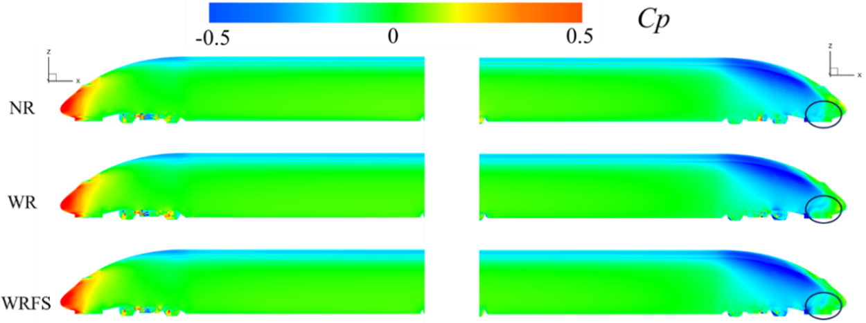
Figure 13: Comparison of time-average pressure distribution at the front and rear of the train

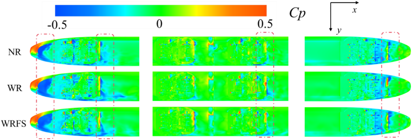
Figure 14: Comparison of time-average pressure distribution at the bottom of the train

Fig. 8 shows the monitoring points selected to detect changes in the flow field as the train passes by. After comparison, data from four monitoring points, namely p6, p9, p10, and p13, were selected for presenting the pressure change of monitoring points, as shown in Fig. 15. The track at the bottom of the train has a very complex influence on the flow field at the bottom of the train, which is the reason for turbulent flow field. Additionally, due to a small area at the bottom of the train, this paper focuses on analyzing at the bottom of the train cowcatcher, behind the first and third bogies, and at the front end of the tail cowcatcher. It can be seen from Fig. 15a–c that there are significant differences in pressure changes near the front of the train as it passes by, mainly reflected in two aspects. One is peak negative pressure, where points p6, p9, and p10 show the same trend in the negative pressure peaks formed near the front of the train (Peak 1, Peak 3, and Peak 5): WR is the largest, followed by WRFS, and NR is the smallest. The other aspect is the positive pressure peak after the negative pressure. It is worth noting that the positive pressure peak only exists in NR (Peak 2). A reasonable explanation is that the WR model impedes the movement of airflow at the bottom of the train to some extent, thus making it easier to form larger negative pressure. In the WRFS model, there are numerous gaps, which weakens the inhibitory effect of the track on the airflow, making the negative pressure peak smaller than that in the WR model. Positive pressure peak does not emerge due to the inhibitory effects of the track and fastening system on the airflow. At p13 on the windward side of the train, the pressure change curve of NR is generally lower than that of WR and WRFS.

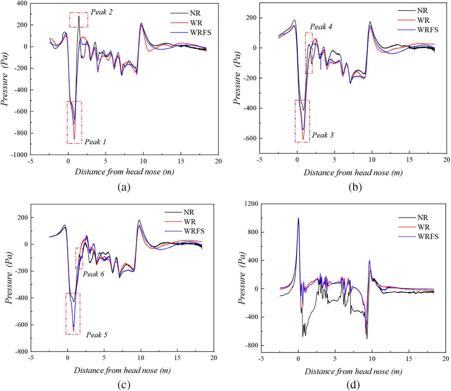
Figure 15: Comparison of pressure at typical monitoring points: (a) p6, (b) p9, (c) p10 and (d) p13

3.2 Train Slipstream Assessment

The train wind generated during high-speed train operation is prone to lifting dust and stones on the ground, posing a threat to the safety of pedestrians and vehicles in the vicinity. The main factors affecting the lifting of objects on the ground are streamwise velocity and spanwise velocity, jointly known as slipstream velocity. Therefore, it is of great importance to analyze the variation of slipstream velocity.

The change in slipstream velocity is more significantly influenced by the track model than that in pressure. Four typical monitoring points are selected in this study, namely bottom monitoring point (p2), monitoring points on the leeward side (p6, p7), and monitoring point on the windward side (p13). Fig. 16 shows the variation of slipstream velocity at four monitoring points under different track models. As can be seen from Fig. 16a, there are four main peaks. For Peaks 1, 2 and 3, WR and WRFS are all less than NR, while for Peak 4, NR is lower than WR and WRFS because the first three peaks are caused by the formation of the train body and bogies. The bottom of the train, the two tracks, and the ground together form a relatively enclosed space, hindering the air flow and thus reducing the peak slipstream velocity. Peak 4, on the other hand, is caused by the wake of the train. At this point, the train has already passed the tracks, with space opened and compressed air released, resulting in greater slipstream velocity. Peak 4 is consistent with the slipstream velocity contour around the train in Fig. 17: WR exhibits the highest slipstream velocity behind the train, successively followed by WRFS and NR, which also confirms the rationality for analyzing slipstream velocity.

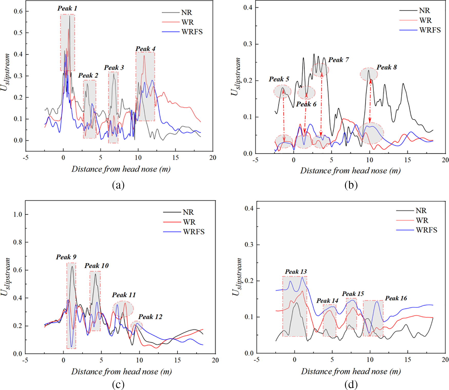
Figure 16: Comparison of slipstream velocity at all monitoring points: (a) p2, (b) p6, (c) p7 and (d) p13

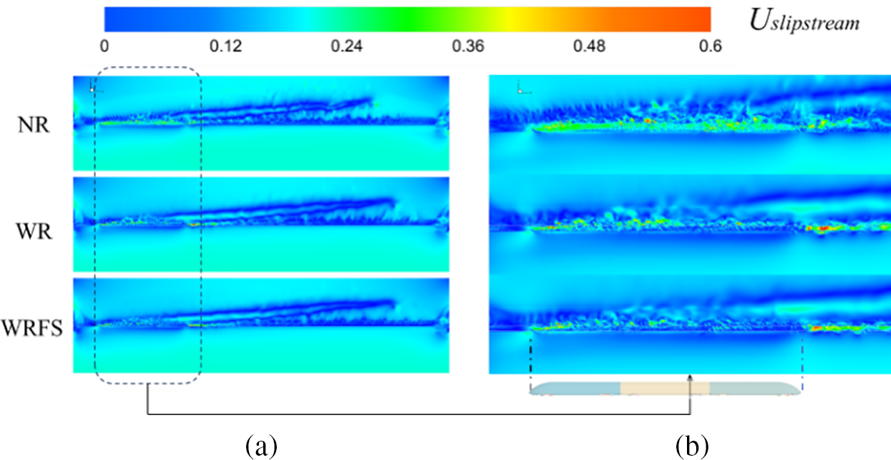
Figure 17: Comparison of slipstream velocity ( Uslipstream ) at plane-z2 (a) overall display (b) Partial enlargement

Fig. 16b,c illustrates the variation of slipstream velocity at monitoring points p6 and p7 on the leeward side of the train. These two monitoring points are located at or near the ground, so the influence of the track model is mainly reflected in the peak values of slipstream velocity, such as Peaks 5, 6 and 7 in Fig. 16b, and Peaks 9 and 10 in Fig. 16c. There are also some differences, especially in the wake of the train. p6, being close to the ground, is most affected by the airflow lateral movement restricted by the track. However, p7, at a certain height above the ground, is less affected. Therefore, the peak slipstream velocity at point p6 in the wake of the train for WR and WRFS is much higher than that for NR, such as Peak 8, with insignificant difference in the peak slipstream velocity at point p7 among the three, such as Peaks 11 and 12.

The variation of slipstream velocity at the windward-side monitoring point p13 is shown in Fig. 16d. It is evident that the curve of slipstream velocity is in the order of WRFS > WR > NR, possibly because the rail and the fastening system obstruct and disrupt the lateral airflow, increasing the slipstream velocity near the track. Therefore, slipstream velocity for the track model with densely complex fastening systems is the highest, successively followed by only rail model, and the model without track.

In addition to establishing monitoring points near the track to monitor the differences in slipstream velocity under three track models, the slipstream velocity contour at the bottom of the train is also provided in Fig. 17. The results clearly show that the slipstream velocity on the leeward side of the train caused by the three models under crosswind conditions have certain angles, as shown in Fig. 18a. According to the color scale of the contour, for WR and WRFS, the longer slipstream shape, the lower velocity of the train. Fig. 17b enlarges the slipstream velocity contour around the train, showing three main differences. Firstly, in terms of the slipstream velocity at the bottom of the train, NR is significantly greater than WR and WRFS; secondly, the slipstream velocity at the rear of the train for WR the highest, successively followed by WRFS and NR, which is consistent with the slipstream velocity observed in Fig. 16a (Peak 4) at the bottom of the train; thirdly, from the perspective of the slipstream velocity on the leeward side of the train, NR is more developed than the other two. This is consistent with the slipstream velocity observed in Fig. 16b,c on the leeward side of the train. The reason for these differences has already been demonstrated at the previous four monitoring points.

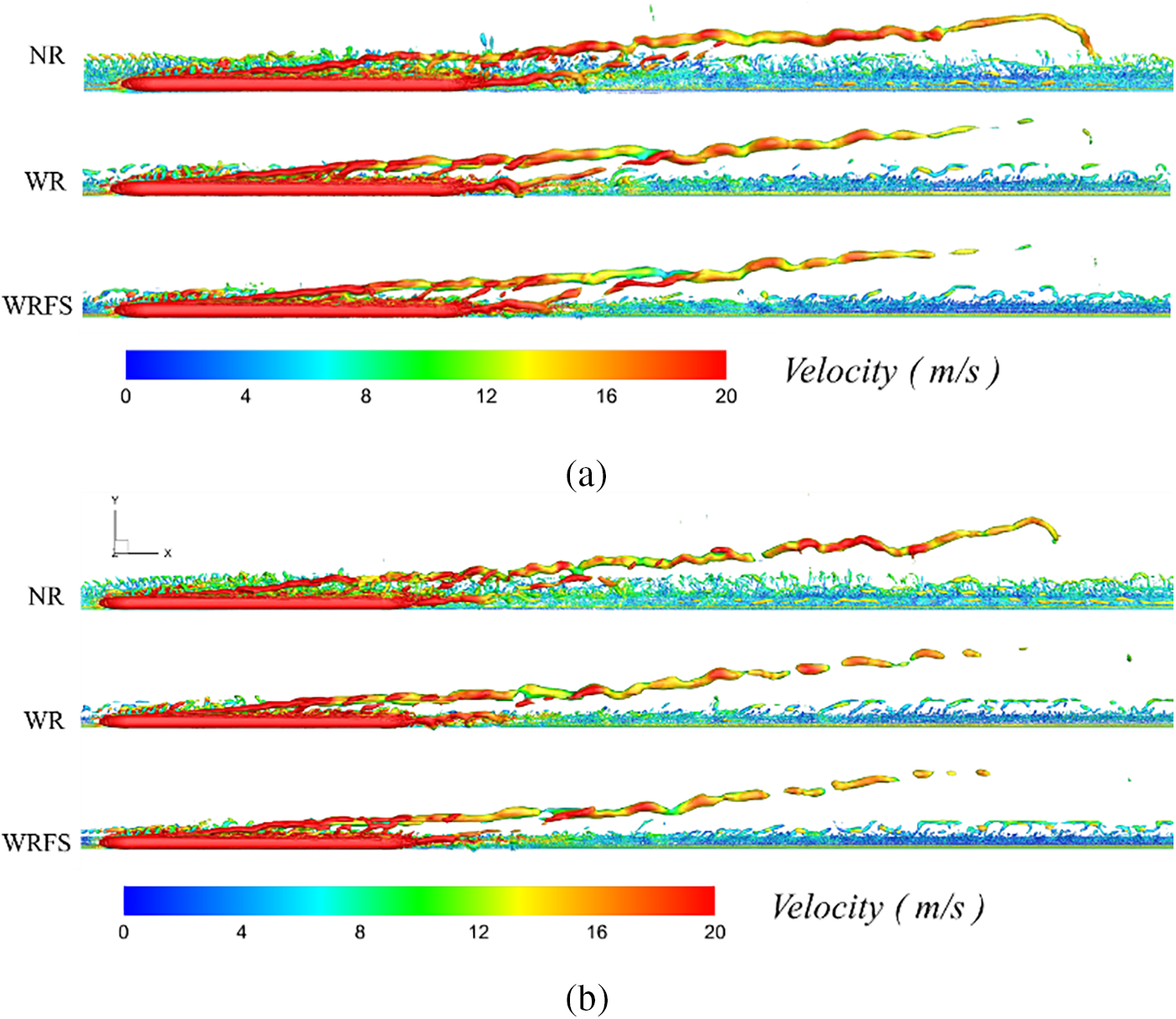
Figure 18: Comparison of instantaneous vortex structures around the train: (a) t = 0.25 s and (b) t = 0.3 s

3.3 Train Wake Flow Analysis

The aerodynamic characteristics of trains is advised to be analyzed from the oscillation of train wake. This section analyzes the vortex structure at the rear of the train, as well as the vorticity in different directions and turbulent kinetic energy. To further explore the reasons for the change in the flow field, the vortex structures are compared and analyzed. Fig. 18 shows isosurface-generated instantaneous vortex structures around the train by the identification criterion called the Q criterion. The Q criterion is expressed as:

Q=0.5∗(∥B∥F2−∥A∥F2) (12)

where ∥B∥F2 denotes the square of the paradigm of the matrix B, which is equivalent to the sum of the squares of all the elements of the matrix B.

And matrix A and matrix B are the symmetric tensor and antisymmetric tensor of velocity gradient:

A=0.5∗(ΔV+ΔVT) (13)

B=0.5∗(ΔV−ΔVT) (14)

where T represents the transpose of the matrix.

Vortex are defined by Q = 2000. To avoid the randomness of instantaneous results, the results for the time of 0.25 and 0.3 s are provided. The differences among the three track models mainly are manifested in two aspects. One is that the vortex structures of WR and WRFS are noticeably shorter than those of NR and the other is that the lateral diffusion of vortex along the track line in NR is more extensive than that in WR and WRFS. The above result is consistent with the analysis result of slipstream velocity in Fig. 17.

In addition, the inclination angle of vortex is also a matter worthy of deeper consideration. According to careful observation and measurement at t = 0.25 s and t = 0.3 s, the vortex of NR is essentially in a straight line, but it is not the case for WR and WRFS, as shown in Fig. 19. The vortex of NR deflects by approximately 3.5–4° compared to the centerline. The vortex of WR and WRFS can be roughly divided into two segments, with the first and second segments respectively having a deflection angle of 2.5–3.2° and 5–7°. Moreover, the degree of deflection in WRFS is greater than that in WR. One reasonable explanation for this is that the presence of the track and fastening system impedes the lateral movement of the airflow around the train, leading to the first inward deflection of the vortices on the lee side of the train; towards the rear right side of the train, without the obstruction of the train, the airflow undergoes a second outward deflection. This corresponds to the inward shift of the negative pressure center observed in plane-x1 in Fig. 11.

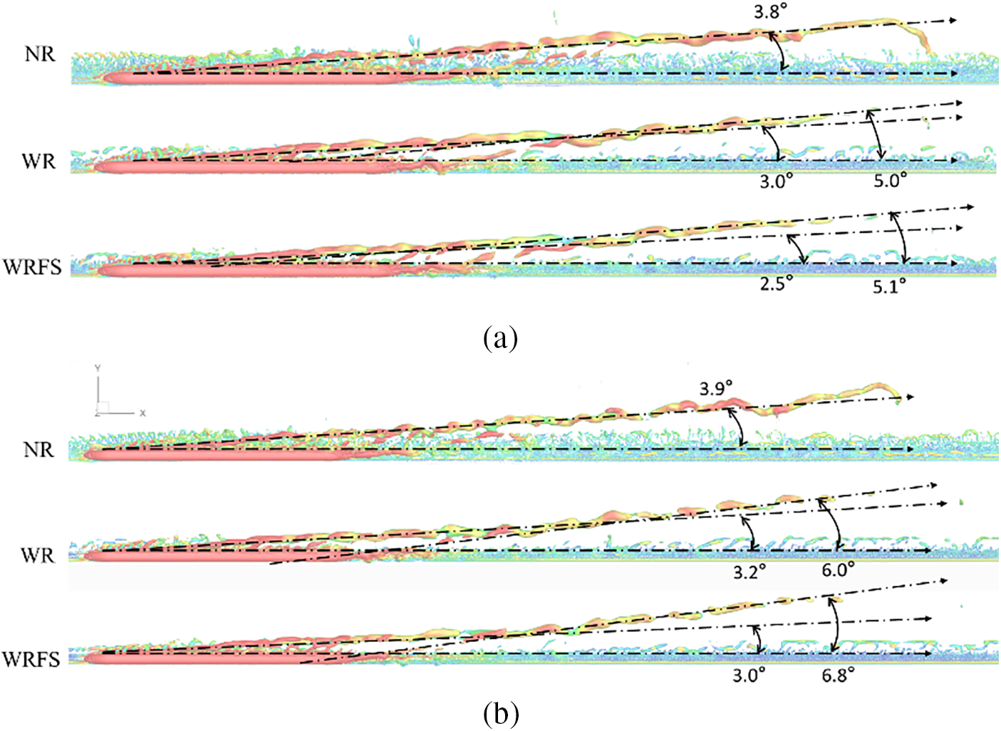
Figure 19: Angle analysis of vortex structure: (a) t = 0.25 s and (b) t = 0.3 s

Fig. 20 compares the Z-direction and Y-direction components of vorticity under three track models. It can be seen from the figure that vortices of different rotational directions alternate. The length of vortices in WR and WRFS is longer than that in NR, but with significantly weaker intensity. The analysis of slipstream velocity earlier indicated that the slipstream velocity of WR and WRFS is smaller than that of NR, so their magnitude of the vorticity component is also slightly smaller. Monitoring point p8 is located on the lee side of the train at a certain distance away, basically in the same plane as the Y-direction vorticity plot. Therefore, vorticity components at monitoring point p8 are compared to verify the variation of vorticity in the train wake. As shown in Fig. 21a,b, positive and negative vorticity are alternately arranged. Moreover, the peak values of vorticity in NR, from Peak 1 to Peak 4 in Fig. 21a and Peak 5 to Peak 6 in Fig. 21b, are all greater than those in WR and WRFS. Additionally, the last peak in the vorticity plot of WR and WRFS emerges later than that in NR. Figs. 20 and 21 mutually corroborate this explanation.

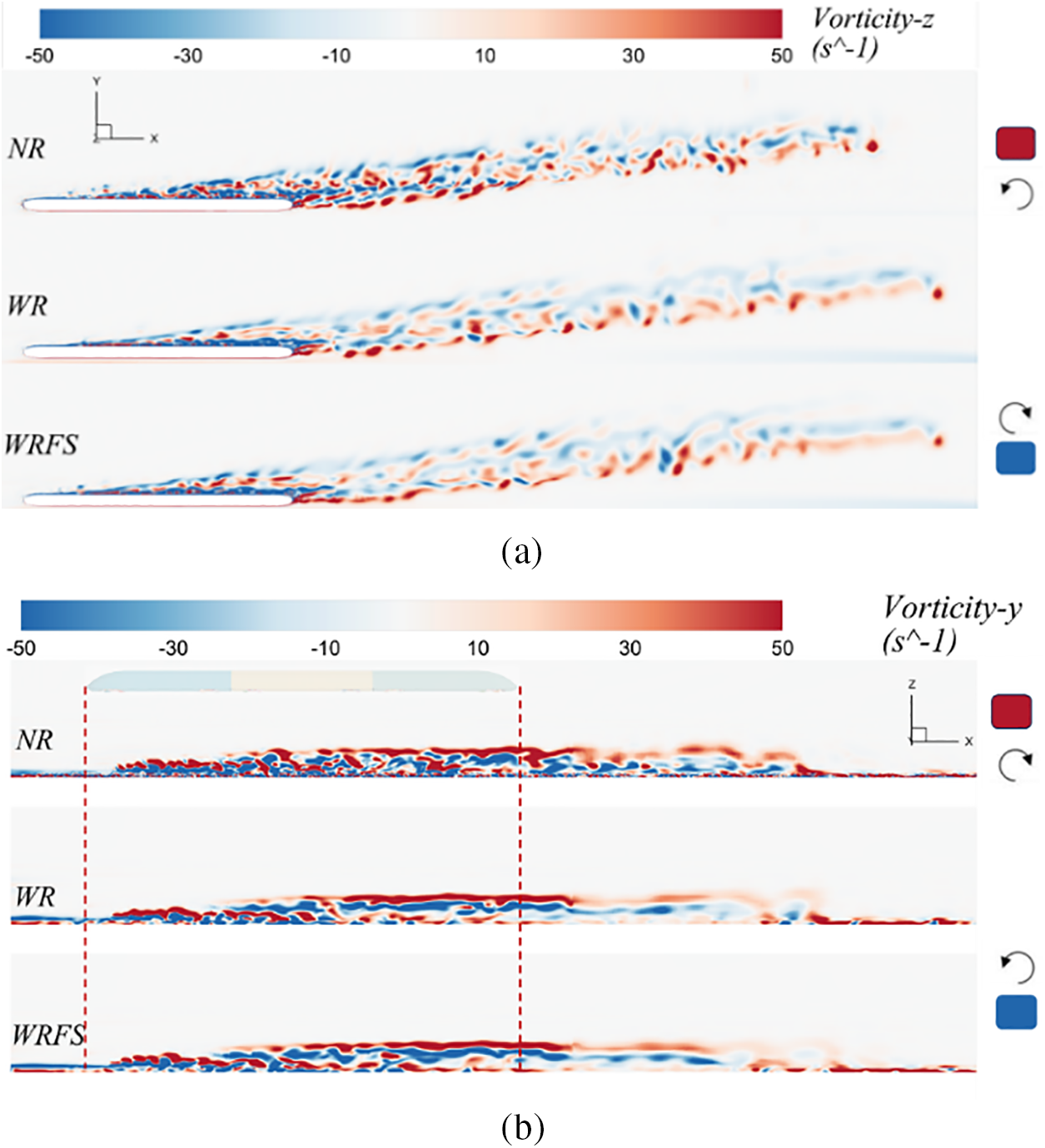
Figure 20: Comparison of the Z-direction and Y-direction components of vorticity: (a) Z-direction and (b) Y-direction

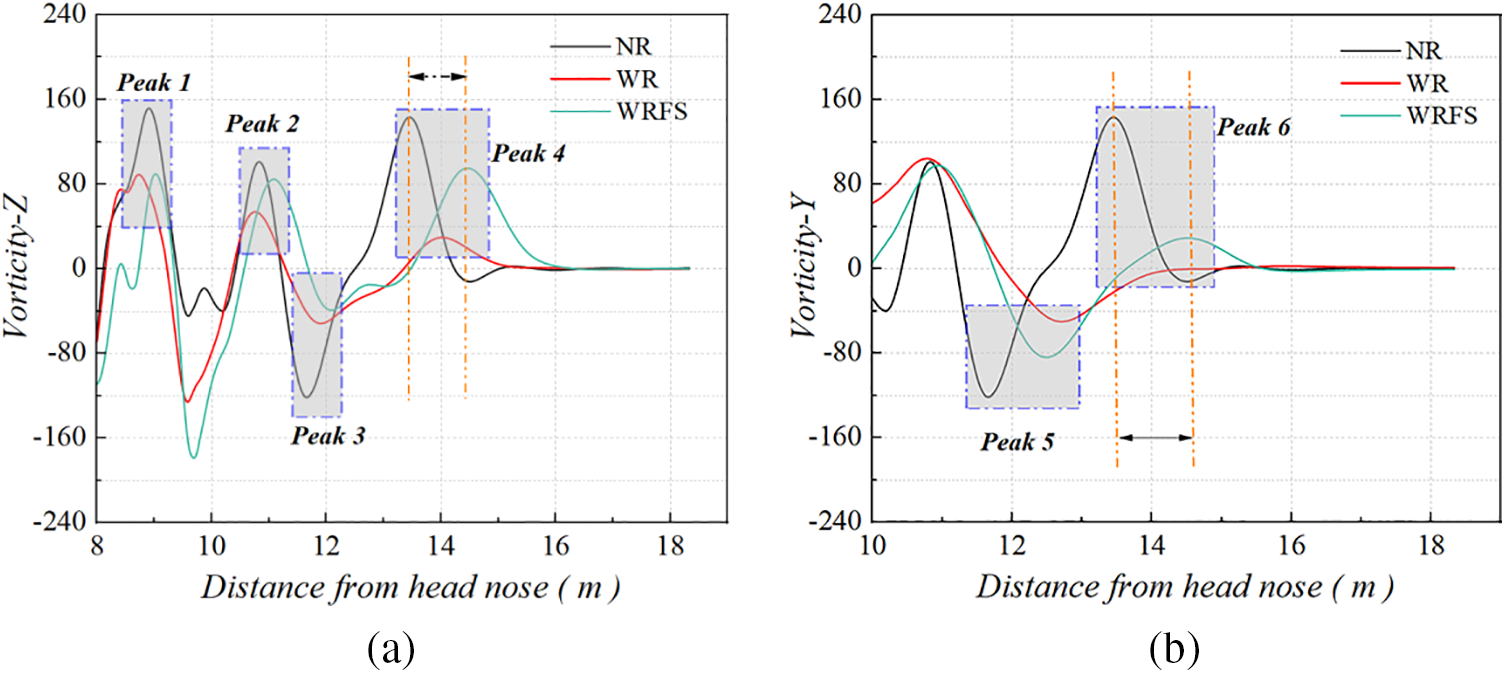
Figure 21: Comparison of vorticity components in Z- and Y-directions at monitoring point p8: (a) Z-direction and (b) Y-direction

Fig. 22 compares vorticity component in the X-direction. The X-section as shown in Fig. 9 is used for display. The large vorticity area generated on the lee side of the train can be visually observed from plane-x1. The distance from the vortex center to the train body is in the order of NR > WR > WRFS. Additionally, lee-side vortices in NR is more extensively developed, which is consistent with the convergence of vortices towards the train, as shown in Fig. 18. The evolution of a pair of shedding vortex at the rear of the train can be observed from plane-x2 and plane-x3. From NR to WR to WRFS, the shedding vortex at the rear of the train approach the ground more closely, and track constraints and fastening system cause the shedding vortex to dissipate more rapidly. Monitoring point 4 is located on the track near the lee side of the train, as shown in Fig. 8. Fig. 23 provides the evolution process of the X-direction vorticity and vorticity magnitude at monitoring point p4 and verifies the evolution process of shedding vortex behind the train. As can be seen from Fig. 23a, the X-direction vorticity of WR and WRFS quickly approaches 0 after the tail of the train, while the vorticity of NR is larger at the same position. The evolution process of vorticity magnitude in Fig. 23b and the length of the slipstream velocity contour in Fig. 17 both confirm that the shedding vortex at the tail of WR and WRFS dissipate more quickly.

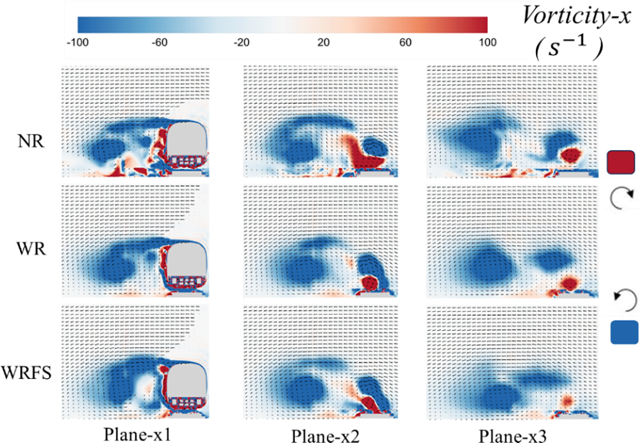
Figure 22: Comparison of the X-direction component of vorticity under different cross-sections

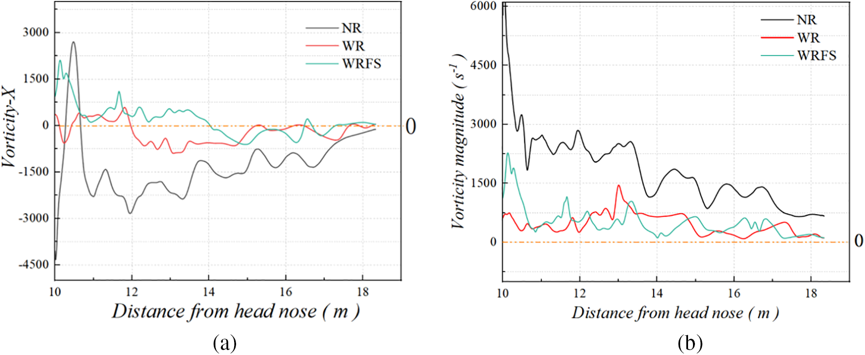
Figure 23: Comparison of vorticity at monitoring point p4: (a) Z-direction component and (b) vorticity magnitude

To clarify the turbulence at the rear of the train, Fig. 24 compares the turbulent kinetic energy at the rear of the train. Near the nose of the train’s tail, the turbulent kinetic energy of NR is much greater than that of WR and WRFS. Based on the variation graph of turbulence intensity monitored at p2, the peak turbulence intensity of NR is much greater than that of WR and WRFS at the nose of the train’s tail. The graph and data mutually confirm each other. Therefore, it can be concluded that the track and the fastening system will help to reduce the turbulence intensity at the nose of the train’s tail under crosswind conditions.

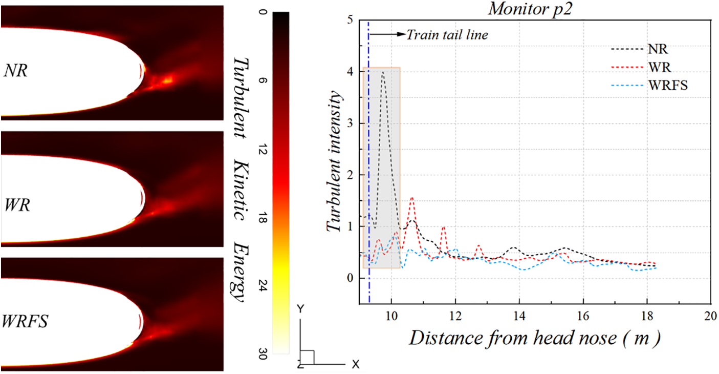
Figure 24: Comparison of turbulent kinetic energy and turbulence intensity at plane-z1

4  Conclusion

The aerodynamic, slipstream velocity, and train wake under three models, namely NR, WR, and WRFS, were compared. The following conclusions are obtained:

1.    Under crosswind condition, track and fastening system reduce the total drag force coefficient of the train by 1.69% but increase the lateral force coefficient of the track model and the fastening system model, respectively by 1.16% and 0.87%. After the establishment of the track model, the oscillation frequency and dominant frequency of drag force coefficient and lateral force coefficient does not significantly change. Moreover, the track and fastening system cause the negative pressure center on the leeward side of the train to shift inward. The aerodynamic forces can be considered virtually unchanged within the error allowance.

2.    In terms of slipstream velocity, the peak slipstream velocity near the ground for WR and WRFS is significantly lower than that for NR. There is little difference in the peak slipstream velocity among NR, WR and WRFS on the leeward side where the rear of the train is away from the ground.

3.    Track and fastening systems affect the deflection of vortex structure of the train. The first inward deflection occurs near the side, and the second deflection behind the tail.

4.    For a pair of shedding vortex at the rear of the train, the track and fastening system accelerate the dissipation of the shedding vortex, thus rapidly reducing turbulence kinetic energy.

In summary, under crosswind conditions, the absence of the track model will have a great impact on the aerodynamic performance, slipstream and wake of high-speed trains, and the flow field obtained is not consistent with the actual one. In contrast, modeling the track, with fastening system included, can capture more details of the flow field and obtain results closer to reality. However, there is no significant difference in the results between WR and WRFS in all aspects. Notably, the fastening system leads to a dramatic increase in the number of grids, which can significantly increase computational cost and time. Conditions permitting, it would be best to employ WRFS. In most cases, the model containing only track (WR) is sufficient for calculations in a trade-off between accuracy and economy.

In this paper, three models regarding railway track have been established to study and comparatively analyze the differences in train aerodynamic forces, slipstreams and wake flow, and the effects of the track and fastening system on the aerodynamic characteristics of the train have been obtained. However, the effect of the track on other aspects of the train is not yet known, such as the effect of whether the track is established on the calculation of the aerodynamic noise of some components of the train, and the effect of the existence of the track on the simulation of sweeping sand at the bottom of the train. These issues are also very important and will be studied as a next step. These issues are explored clearly, which can provide a certain basis for various aspects of research track modeling.

Acknowledgement: None.

Funding Statement: The authors disclosed receipt of the following financial support for the research, authorship and/or publication of this article: This work was funded by the National Natural Science Foundation of China (Grant No. 12172308).

Author Contributions: Yuzhe Ma: Writing—Original Draft, Data Curation, Methodology, Validation, Visualization. Jiye Zhang: Writing—Review & Editing, Funding Acquisition. Jiawei Shi: Conceptualization, Writing—Review & Editing. All authors reviewed the results and approved the final version of the manuscript.

Availability of Data and Materials: Data and materials for this paper are available from the corresponding author upon request.

Ethics Approval: Not applicable.

Conflicts of Interest: The authors declare no conflicts of interest to report regarding the present study.

References

1. Pope CW. Effective management of risk from slipstream effects at trackside and platforms. In: Rail Safety and Standards Board—T425 report. UK: Rail Safety and Standards Board; 2007. [Google Scholar]

2. CEN European Standard. Railway applications—aerodynamics—part 4: requirements and test procedures for aerodynamics on open track. 2009. SR EN 14067-4+A1. Available from: https://www.bsigroup.com. [Accessed 2024]. [Google Scholar]

3. CEN European Standard. Railway applications—aerodynamics—part 6: requirements and test procedures for cross wind assessment. 2010. EN 14067-6. Available from: https://www.bsigroup.com. [Accessed 2024]. [Google Scholar]

4. CEN European Standard. Railway applications—aerodynamics—part 4: requirements and test procedures for aerodynamics on open track. 2013. EN 14067-4. Available from: https://www.bsigroup.com. [Accessed 2024]. [Google Scholar]

5. Baker C. The flow around high speed trains. J Wind Eng Ind Aerodyn. 2010;98(6–7):277–98. doi:10.1016/j.jweia.2009.11.002. [Google Scholar] [CrossRef]

6. Bell JR, Burton D, Thompson M, Herbst A, Sheridan J. Wind tunnel analysis of the slipstream and wake of a high-speed train. J Wind Eng Ind Aerodyn. 2014;134(4):122–38. doi:10.1016/j.jweia.2014.09.004. [Google Scholar] [CrossRef]

7. Cheli F, Corradi R, Rocchi D, Tomasini G, Maestrini E. Wind tunnel tests on train scale models to investigate the effect of infrastructure scenario. J Wind Eng Ind Aerodyn. 2010;98(6–7):353–62. doi:10.1016/j.jweia.2010.01.001. [Google Scholar] [CrossRef]

8. Jönsson M, Wagner C, Loose S. Particle image velocimetry of the underfloor flow for generic high-speed train models in a water towing tank. Pro Inst Mech Eng, Part F: J Rail Rapid Transit. 2014;228(2):194–209. doi:10.1177/0954409712470607. [Google Scholar] [CrossRef]

9. Wang S, Burton D, Herbst AH, Sheridan J, Thompson MC. The impact of rails on high-speed train slipstream and wake. J Wind Eng Ind Aerodyn. 2020;198(6):104114. doi:10.1016/j.jweia.2020.104114. [Google Scholar] [CrossRef]

10. Bell JR, Burton D, Thompson MC, Herbst AH, Sheridan J. Flow topology and unsteady features of the wake of a generic high-speed train. J Fluid Struct. 2016;61(4):168–83. doi:10.1016/j.jfluidstructs.2015.11.009. [Google Scholar] [CrossRef]

11. Wang S, Burton D, Herbst A, Sheridan J, Thompson MC. The effect of bogies on high-speed train slipstream and wake. J Fluid Struct. 2018;83(6):471–89. doi:10.1016/j.jfluidstructs.2018.03.013. [Google Scholar] [CrossRef]

12. Paz C, Suárez E, Gil C. Numerical methodology for evaluating the effect of sleepers in the underbody flow of a high-speed train. J Wind Eng Ind Aerodyn. 2017;167:140–7. doi:10.1016/j.jweia.2017.04.017. [Google Scholar] [CrossRef]

13. Wang S, Bell JR, Burton D, Herbst AH, Sheridan J, Thompson MC. The performance of different turbulence models (URANS, SAS and DES) for predicting high-speed train slipstream. J Wind Eng Ind Aerodyn. 2017;165(6):46–57. doi:10.1016/j.jweia.2017.03.001. [Google Scholar] [CrossRef]

14. Soper D, Baker C, Jackson A, Milne DR, Le Pen L, Watson G, et al. Full scale measurements of train underbody flows and track forces. J Wind Eng Ind Aerodyn. 2017;169(1):251–64. doi:10.1016/j.jweia.2017.07.023. [Google Scholar] [CrossRef]

15. Tschepe J, Nayeri CN, Paschereit CO. On the influence of Reynolds number and ground conditions on the scaling of the aerodynamic drag of trains. J Wind Eng Ind Aerodyn. 2021;213(1202):104594. doi:10.1016/j.jweia.2021.104594. [Google Scholar] [CrossRef]

16. Rochard BP, Schmid F. A review of methods to measure and calculate train resistances. Proc Inst Mech Eng, Part F: J Rail Rapid Transit. 2000;214(4):185–99. doi:10.1243/0954409001531306. [Google Scholar] [CrossRef]

17. Dorigatti F, Sterling M, Baker CJ, Quinn AD. Crosswind effects on the stability of a model passenger train–a comparison of static and moving experiments. J Wind Eng Ind Aerodyn. 2015;138:36–51. doi:10.1016/j.jweia.2014.11.009. [Google Scholar] [CrossRef]

18. He XH, Zou YF, Wang HF, Han Y, Shi K. Aerodynamic characteristics of a trailing rail vehicles on viaduct based on still wind tunnel experiments. J Wind Eng Ind Aerodyn. 2014;135(8):22–33. doi:10.1016/j.jweia.2014.10.004. [Google Scholar] [CrossRef]

19. Tomasini G, Giappino S, Corradi R. Experimental investigation of the effects of embankment scenario on railway vehicle aerodynamic coefficients. J Wind Eng Ind Aerodyn. 2014;131(1):59–71. doi:10.1016/j.jweia.2014.05.004. [Google Scholar] [CrossRef]

20. Premoli A, Rocchi D, Schito P, Tomasini G. Comparison between steady and moving railway subjected to crosswind by CFD analysis. J Wind Eng Ind Aerodyn. 2016;156(5):29–40. doi:10.1016/j.jweia.2016.07.006. [Google Scholar] [CrossRef]

21. Hemida H, Baker CJ. Large-eddy simulation of the flow around a freight wagon subjected to a crosswind. Comput & Fluids. 2010;39(10):1944–56. doi:10.1016/j.compfluid.2010.06.026. [Google Scholar] [CrossRef]

22. Shao XM, Wan J, Chen DW, Xiong HB. Aerodynamic modeling and stability analysis of a high-speed train under strong rain and crosswind conditions. J. Zhejiang Univ Sci A. 2011;12(12):964–70. doi:10.1631/jzus.A11GT001. [Google Scholar] [CrossRef]

23. Krajnović S, Ringqvist P, Nakade K, Basara B. Large eddy simulation of the flow around a simplified train moving through a crosswind flow. J Wind Eng Ind Aerodyn. 2012;110(3):86–99. doi:10.1016/j.jweia.2012.07.001. [Google Scholar] [CrossRef]

24. Giappino S, Rocchi D, Schito P, Tomasini G. Cross wind and rollover risk on lightweight railway vehicles. J Wind Eng Ind Aerodyn. 2016;153(8):106–12. doi:10.1016/j.jweia.2016.03.013. [Google Scholar] [CrossRef]

25. Niu J, Wang Y, Liu F, Li R. Numerical study on comparison of detailed flow field and aerodynamic performance of bogies of stationary train and moving train. Veh Syst Dyn. 2021;59(12):1844–66. doi:10.1080/00423114.2020.1794015. [Google Scholar] [CrossRef]

26. Wang J, Wang T, Yang M, Qian B, Zhang L, Tian X, et al. Research on the influence of different heating zone lengths on pressure waves and a newly designed method of pressure wave mitigation in railway tunnels. Tunnelling Undergr Space Technol. 2022;122(10):104379. doi:10.1016/j.tust.2022.104379. [Google Scholar] [CrossRef]

27. Sun Z, Zhang Y, Guo D, Yang G, Liu Y. Research on running stability of CRH3 high speed trains passing by each other. Eng Appl Comput Fluid Mech. 2014;8(1):140–57. doi:10.1080/19942060.2014.11015504. [Google Scholar] [CrossRef]

28. Chu CR, Chien SY, Wang CY, Wu TR. Numerical simulation of two trains intersecting in a tunnel. Tunnelling Undergr Space Technol. 2014;42(8):161–74. doi:10.1016/j.tust.2014.02.013. [Google Scholar] [CrossRef]

29. Wang K, Xiong X, Wen C, Li X, Chen G, Chen Z, et al. Impact of the train heights on the aerodynamic behaviour of a high-speed train. Eng Appl Comput Fluid Mech. 2023;17(1):2233614. doi:10.1080/19942060.2023.2233614. [Google Scholar] [CrossRef]

30. Reyes CEA, Rocchi D, Tomasini G, Sánchez MI, Artano M. Effects of different aerodynamic configurations on crosswind stability of a conventional train. J Wind Eng Ind Aerodyn. 2023;242:105588. doi:10.1016/j.jweia.2023.105588. [Google Scholar] [CrossRef]

31. Huo X, Liu T, Chen Z, Li W, Gao H. Effect of the formation type with different freight vehicles on the train aerodynamic performance. Veh Syst Dyn. 2022;60(11):3868–96. doi:10.1080/00423114.2021.1981951. [Google Scholar] [CrossRef]

32. Sun Z, Yao S, Yang G. Research on aerodynamic optimization of high-speed train’s slipstream. Eng Appl Comput Fluid Mech. 2020;14(1):1106–27. doi:10.1080/19942060.2020.1810128. [Google Scholar] [CrossRef]

33. Guo Z, Liu T, Hemida H, Chen Z, Liu H. Numerical simulation of the aerodynamic characteristics of double unit train. Eng Appl Comput Fluid Mech. 2020;14(1):910–22. doi:10.1080/19942060.2020.1784798. [Google Scholar] [CrossRef]

34. Luo J, Wang L, Shang S, Li F, Guo D, Gao L, et al. Study of unsteady aerodynamic performance of a high-speed train entering a double-track tunnel under crosswind conditions. J Fluid Struct. 2023;118(8):103836. doi:10.1016/j.jfluidstructs.2023.103836. [Google Scholar] [CrossRef]

35. Shi J, Zhang J. Effect of bogie cavity end wall inclination on flow field and aerodynamic noise in the bogie region of high-speed trains. Comput Model Eng Sci. 2024;139(2):2175–95. doi:10.32604/cmes.2023.043539. [Google Scholar] [CrossRef]

36. Cai L, Lou Z, Liu N, An C, Zhang J. Numerical investigation of the deposition characteristics of snow on the bogie of a high-speed train. Fluid Dyn Mater Process. 2020;16(1):41–53. doi:10.32604/fdmp.2020.07731. [Google Scholar] [CrossRef]

37. Liu M, Wang J, Zhu H, Krajnovic S, Gao G. A numerical study of snow accumulation on the bogies of high-speed trains based on coupling improved delayed detached eddy simulation and discrete phase model. Pro Inst Mech Eng, Part F: J Rail Rapid Transit. 2019;233(7):715–30. doi:10.1177/0954409718805817. [Google Scholar] [CrossRef]

38. Wang Y, Wang T, Jiang C, Wu Y, Zhao C, Shi F, et al. Numerical study on slipstream-induced snow drifting and accumulation in the bogie region of a high-speed train passing the snowy ballast bed. J Wind Eng Ind Aerodyn. 2023;232(3):105269. doi:10.1016/j.jweia.2022.105269. [Google Scholar] [CrossRef]

39. Xia C, Shan X, Yang Z. Comparison of different ground simulation systems on the flow around a high-speed train. Proc Inst Mech Eng, Part F: J Rail Rapid Transit. 2017;231(2):135–47. doi:10.1177/0954409715626191. [Google Scholar] [CrossRef]

40. Bell JR, Burton D, Thompson MC, Herbst AH, Sheridan J. Moving model analysis of the slipstream and wake of a high-speed train. J Wind Eng Ind Aerodyn. 2015;136(2):127–37. doi:10.1016/j.jweia.2014.09.007. [Google Scholar] [CrossRef]