High-Order DG Schemes with Subcell Limiting Strategies for Simulations of Shocks, Vortices and Sound Waves in Materials Science Problems

Nomenclature

1  Introduction

The shock wave is a compression wave in which the pressure, density, and temperature undergo sudden changes on the wavefront in gas, liquid and solid media. There are various potential applications of shock waves in the materials science processes. For instance, in the shock wave synthesis of nanomaterials, the shock wave can be utilized to induce rapid compression and heating of a precursor material, often in a solution or suspension, leading to the formation of nanomaterials. In explosive welding, the shock waves generated by detonating explosives are used to join metal plates, which can be applied in tube and pipe fabrication. The shock wave created by a pulsed laser can be used in the technique of laser-induced forward transfer (LIFT), which has potential application in the area of microfabrication or bioprinting. In medical treatment, the shock wave can be utilized to fragment kidney stones or enhance drug delivery. The extremely high pressures and temperatures produced of the compressed gases produced by the shock wave can be employed in studying the material behavior and forming complex shapes or hard-to-deform materials. The rapid compression of the shock wave can lead to chemical reactions, phase transitions, and changes in material properties, which are also related to the propulsion and energy applications like fuel injection and inertial confinement fusion. The applications of shock waves are also seen in the area of shock wave processing of ceramics, shock wave-induced phase transitions, hydrodynamic cavitation, etc. The shock waves and vortices are two fundamental flow structures. The interaction between shock waves and vortices is a major contributor to aeroacoustic phenomena. It has been one of the most significant and difficult tasks to develop numerical schemes in computational aeroacoustics, especially for complex nonlinear phenomena like shock-vortex interactions.

To simulate aeroacoustic phenomena that are related to a shock or discontinuity, the classical centered schemes [1,2] usually fail to capture the discontinuity without spurious oscillations. Since the capturing of sound generation essentially necessitates a numerical scheme with low artificial dissipation, many researchers thus seek high-order and high-resolution schemes, such as weighted essentially non-oscillatory (WENO) methods and compact finite difference methods that have been applied to study acoustic problems including shock-vortex interactions, see for instance [3,4]. For WENO methods, although the shocks are well-captured, a large number of mesh points is often needed due to the excessive numerical dissipation for acoustics computations. For compact finite difference methods, nonlinear limiters are required in case of strong shock waves. There have been abundant works devoted to developing numerical schemes with a minimum of numerical dispersion and dissipation that are applicable for shock-associated noise problems. For instance, the authors in [5] have developed a hybrid scheme that is suitable for compressible turbulence problems. Some of the high-order schemes are suggested and improved for the shock problems and the noise problems, such as the weighted compact nonlinear scheme in [6], the optimized weighted essentially non-oscillatory scheme in [7], the optimized compact scheme in [8], the modified monotonicity-preserving scheme in [9], the upwind multi-layer compact scheme in [10] and the compact gas-kinetic scheme in [11]. Most of them have been done in the finite difference and finite volume discretization framework.

Another type of high order schemes that originate from a class of finite element methods utilizes the discontinuous piecewise function representation within each element. The discontinuous Galerkin (DG) method [12] is one of the typical representatives. In computational aeroacoustics, previous studies in the literature have mainly concentrated on theoretical and numerical analysis of propagation properties of DG schemes, such as the dispersion and dissipation behavior analysis in [13–15], error and superconvergence properties analysis in [16,17], etc. More recently, the propagation properties of DG schemes have been studied in comparison with finite difference schemes in [18]. There are also various applications of DG-like schemes to computational aeroacoustics, see for instance [19–23]. Nevertheless, compared to the WENO schemes, the high-order DG schemes have been relatively less applied to the simulation of complex shock-associated noise problems, which is done by directly solving the Navier-Stokes (NS) equations.

Motivated by the desire to simulate shock-associated noise problems, this work presents a high-order subcell limiting-based DG method for aeroacoustic computations. By switching to the FV discretization on an embedded sub-cell grid, the method possesses the advantages in both DG high accuracy characteristic and FV shock-capturing capability. We utilize a class of high-fidelity FV schemes that are designed for the capture of both discontinuities and small-scale flow structures, see for instance [24]. The resulting method is therefore able to resolve discontinuities and multi-scale structures for shocked flows [25]. In this work, the DG methods up to the 6th-order accuracy have been applied to aeroacoustic computations involving shocks, vortices and sound waves, which to the best of the authors’ knowledge, has been rarely seen for utilizing such high-order DG scheme in computational aeroacoustics for strong shock-vortex interactions.

The rest of the article is organized as follows. Section 2 briefly introduces the governing equation and the DG/FV method applied in this work. Section 3 describes numerical results, including benchmark tests for the Euler equations and complex flow simulations for the NS equations. Some conclusions are drawn in Section 4.

2  The Governing Equation and the Discretization Method

2.1 Governing Equations

The compressible NS equations are written as

∂ρ∂t+∇⋅(ρu)=0∂ρu∂t+∇⋅(ρu+pδ_−τ_)=0∂ρe∂t+∇⋅(ρeu+(pδ_−τ_)⋅u−κ∇T)=0 (1)

By omitting the viscous stress tensor τ_ and the heat flux κ∇T , the Euler equations can be obtained from the above equations. In Eq. (1), t is the time, ρ is the density, p is the static pressure, u is the velocity vector, T is the temperature, e is the total energy per unit mass and δ_ is the Kronecker tensor. We have the viscous stress tensor expressed as

τ_=μ(∇u+(∇u)T−23(∇⋅u)δ_) (2)

with μ denoting the molecular dynamic viscosity. The system of equations is completed by adding the state equation for a perfect gas

p=(γ−1)ρ(e−12u⋅u) (3)

where γ is the ratio of the specific heats.

2.2 Discontinuous Galerkin and Finite Volume Discretizations

The Eq. (1) is rewritten as a conservative form to formulate the DG method, and thus reads

∂Q∂t+∇⋅Fc(Q)−∇⋅Fv(Q,∇Q)=0 (4)

where Q is the conservative state vector, Fc(Q) is the inviscid flux tensor and Fv(Q,∇Q) is the viscous flux tensor. By introducing the approximation solution Qh and test function vh , the final DG discretization equations can be written as

∫Kνh∂Qh∂tdΩ+∫∂Kνh(Fc(Qh)−Fv(Qh,∇Qh))⋅n→dσ−∫K∇νh⋅(Fc(Qh)−Fv(Qh,∇Qh))dΩ=0 (5)

Eq. (5) is obtained by integrating over the element K and performing an integration by parts. In Eq. (5), n→ is the outward unit normal vector to the boundary. In the DG method, the inviscid flux Fc⋅n→ is replaced by a monotone Riemann flux function and the local Lax–Friedrichs flux [12] is adopted in this work. The viscous flux is approximated by the second scheme of Bassi and Rebay (BR2) [26]. The DG solution is expressed in the following form:

Qh=∑l=1N(p)νh,lQl(t) (6)

where N(p) is the number of modes and Ql is the degrees of freedom (DoFs). We use the Legendre polynomials as the test function. For the domain and boundary integrals in Eq. (5) we utilize the Gauss-Legendre quadrature points.

Similar to the DG discretization described above, we also rewrite the governing equation of Eq. (1) as the conservative form for the FV discretization. To better distinguish the DG and FV discretization, the solution and flux is denoted by q and f in the FV method. As a result, the integration formulation of Eq. (4) for the FV discretization reads

∫K∂q∂tdΩ+∫K(∇⋅fc(q)−∇⋅fv(q,∇q))dΩ=0 (7)

Currently the FV discretization is carried out on the structured meshes that have conforming elements denoted by

Kij=[xi−1/2,xi+1/2]×[yj−1/2,yj+1/2] (8)

Eq. (8) is integrated over element Kij to obtain

dq¯ij(t)dt+f^c,ij+1/2−f^c,ij−1/2=f^v,ij+1/2−f^v,ij−1/2 (9)

with cell average value q¯ij expressed as

q¯ij(t)=1Ωij∫xi−1/2xi+1/2∫yj−1/2yj+1/2q(x,y,t)dydx (10)

where Ωij is the cell volume. We use ij±1/2 that includes i±1/2,j and i,j±1/2 to indicate both x and y components. f^c,ij+1/2 and f^c,ij−1/2 are convective numerical flux and f^v,ij+1/2 and f^v,ij−1/2 are viscous numerical flux. The same local Lax–Friedrichs flux [12] is adopted for the convective flux computation and for the viscous flux computation the second-order central difference is employed. The high-order central difference can also be applied in the discretization of the viscous flux for the FV method, although it involves the high-order approximation of the variables and the derivates of the variables on the subcell interface. Further research is needed to determine whether the use of the higher-order method for the FV discretization of the viscous flux will make an obvious impact on the computational results of the present method, which is beyond the scope of this work.

The final semi-discrete form of Eqs. (5) and (9) are formulated as

MdQdt+R(Q)=0 anddq¯dt+r(q¯)=0 (11)

for the DG and FV discretization, respectively. M denotes the mass matrix in the DG method. R(Q) and r(q¯) are the corresponding residual vectors. The semi-discrete systems of equations are then discretized with a third order version of TVD Runge–Kutta method [12] for both DG and FV discretizations.

This work presents the subcell-limiting-based DG method that switches to the FV discretization on an embedded sub-cell grid for shock-capturing. Each computational element is also called as the main element. The subcells are embedded within the main element. In this work, we equally divide the main element into the subcells. The number of the subcells in each main element is equal to the number of DoFs used in the DG scheme. The following Section 2.3 will provide the details of the reconstruction procedure in the FV method performed on the subcell and the connection between the FV subcell solution and DG main element solution.

2.3 DG Schemes with Subcell Limiting Strategies

2.3.1 Subcell Limiting Strategies Built upon High-Fidelity Shock-Capturing Schemes

The subcell limiting method is one of the existing strategies to capture shocks and discontinuities for the DG method. The general idea is to construct the so-called subcells in the DG main elements and apply the mature shock-capturing schemes on those subcells that are usually around a discontinuity or large gradient. Since most mature shock-capturing schemes have been developed within the FV or FD framework, the limiting on the subcells is often taken by the FV or FD method [27–31]. Currently in this study, the FV method is adopted. The FV reconstruction scheme is implemented dimension-by-dimension. We only compute the numerical flux at the center point of the subcell interfaces in the FV method. The values of the variables on the left and right side of the subcell interfaces are obtained by one reconstruction process along each dimensional direction. Our suggested approach is built upon the boundary variation diminishing (BVD) reconstruction paradigm [32]. A class of high-fidelity schemes denoted as the PnTm [24] is utilized as FV subcell limiting strategies, which achieve better subcell resolution and lower numerical diffusion properties for shocked flows [25]. Here the PnTm (polynomial of n-degree and THINC function of m-level) is a shock capturing scheme designed by employing linear-weight polynomials and THINC (Tangent of Hyperbola for INterface Capturing) [33] functions as reconstruction candidates. For instance, the P4T2 scheme adopted in this work employs a 4th-degree linear-weight polynomial q~iP4 that reads

qi−1/2R,P4=q˜iP4(xi−1/2)=130q¯i+2−1360q¯i+1+4760q¯i+920q¯i−1−120q¯i−2 (12)

qi+1/2L,P4=q˜iP4(xi+1/2)=130q¯i−2−1360q¯i−1+4760q¯i+920q¯i+1−120q¯i+2 (13)

The qi−1/2R and qi+1/2L are the reconstructed right-side value on the interface i−1/2 and left-side value on the interface i + 1/2, respectively. The P4T2 scheme also employs a THINC function q~iT that reads

q~iT(x)=q¯min+q¯max2[1+θtanh⁡(β(x−xi−1/2xi+1/2−xi−1/2−x~i))] (14)

The THINC function in Eq. (14) is a piecewise, non-polynomial function. The most important parameter in the THINC function is β which controls the jump steepness. The P4T2 scheme adopts the THINC function with 2 level jump steepness controlled by β1 = 1.1 and β2 = 1.6. The THINC formulas are well documented in for instance [24,25,33]. In Eq. (14), q¯min=min(q¯i−1,q¯i+1),q¯max=max(q¯i−1,q¯i+1)−q¯min , and θ=sgn(q¯i+1−q¯i−1) . x~i can be computed using the constraint condition

q¯i=1Δx∫xi−1/2xi+1/2qi(x)dx (15)

The reconstructed values by the THINC function on the left side of interface i + 1/2 read

qi+1/2L,T,β=q¯min+q¯max2[1+θtanh⁡(β)+A1+Atanh⁡(β)] (16)

and on the right side of interface i − 1/2

qi−1/2R,T,β=q¯min+q¯max2(1+θA) (17)

In Eqs. (16) and (17) we have

A=B/cosh(β)−1tanh⁡(β),B=exp⁡(θβ(2C−1)),C=q¯i−q¯min+εq¯max+ε,ε=10−20 (18)

Having described the 4th-degree linear-weight polynomial in Eqs. (12), (13) and the THINC function in Eq. (14), we then present the strategy to determine the final function for cell i by choosing from q~iP4 and q~iT . The strategy is known as multi-stage BVD algorithm [24]. Specifically, a 2-stage method of BVD algorithm is adopted in this study. The method initially sets the reconstruction function with q~iP4 for all cells, then calculates the total boundary variation (TBV) values of q~iP4 and q~iT,β1 (THINC function with β1 = 1.1) as

TBViP4=|qi−1/2L,P4−qi−1/2R,P4|+|qi+1/2L,P4−qi+1/2R,P4| (19)

and

TBViT,β1=|qi−1/2L,T,β1−qi−1/2R,T,β1|+|qi+1/2L,T,β1−qi+1/2R,T,β1| (20)

The reconstruction function for cell i at the first stage, denoted as q~i<1> , is determined by the following BVD algorithm

q~i<1>={q~iT,β1if TBVi−1T,β1<TBVi−1P4 or TBViT,β1<TBViP4 or TBVi+1T,β1<TBVi+1P4,q~iP4otherwise (21)

which means the reconstruction function is chosen to be THINC function if the TBV values of THINC function is smaller at either cell i or at one of its neighboring cells. Otherwise, the reconstruction function will maintain the initial choice of q~iP4 .

After the reconstruction function is chosen for all cells by the first stage of BVD algorithm, the method then calculates the TBV values of q~i<1> and q~iT,β2 (THINC function with β2 = 1.6) using similar formula as Eqs. (19) and (20) as

TBVi<1>=|qi−1/2L,<1>−qi−1/2R,<1>|+|qi+1/2L,<1>−qi+1/2R,<1>| (22)

and

TBViT,β2=|qi−1/2L,T,β2−qi−1/2R,T,β2|+|qi+1/2L,T,β2−qi+1/2R,T,β2| (23)

The final reconstruction function is determined at the second stage, denoted as q~i<2> for cell i, as

q~i<2>={q~iT,β2if TBViT,β2<TBVi<1>,q~i<1>otherwise (24)

We mention the above procedure can also be done in multi-stage BVD selection algorithm by introducing dissipation-adjustable method to achieve even less dissipative schemes [34].

2.3.2 FV Subcell Limiting Strategies for High-Order DG Methods

The last subsection gives the details of the P4T2 scheme that is utilized as FV subcell limiting strategies. In this subsection, we will present the approach to implement the FV subcell limiting in the DG method.

We start with Eq. (11) where the equations of DG or FV methods will be discretized by the RK scheme. First, before the RK iteration process starts, we would like to bridge the FV subcell solution and the DG main element solution. The specific choice on how the main element is divided into subcells as well as the definition of the FV solution on these subcells will determine the connection between the DG and FV solutions. For dividing the main element into subcells, there are uniform and nonuniform subdivisions. For defining the subcell solution, there are Gauss quadrature point values or cell averaged values used in the definition. The subcell number can also be chosen as equal to or larger than the number of degrees of freedom of the DG method. Our method is to equally divide the main element into subcells with the subcell number equal to DG degrees of freedom. FV solutions are obtained by

q¯Kij=1Ωij∫xi−1/2xi+1/2∫yj−1/2yj+1/2Qh(x,y,t)dydx (25)

where the structured index of the subcell within main element K is denoted by ij. Based on Eq. (25) we compute and store the transformation matrices to obtain the FV subcell solution from a DG solution representation. Obviously, the reverse matrices are used to obtain the DG solution from a FV subcell solution representation. From Eq. (21) both matrices have dimension of N(p) × N(p) where N(p) is also the subcell number in this work.

Then we begin the iteration process with the RK method. During each stage of a time step in the RK method, the present approach solves the systems of Eq. (11) through the following four main steps:

Step 1 is to identify the so-called FV cells that are about to perform the FV computation. We exploit the reconstruction candidates used in the P4T2 scheme, i.e., a 4th-degree linear-weight polynomial q~iP4 and a THINC function q~iT,β1 with β = 1.1. The TBV values of q~iP4 minus the TBV values of q~iT,β1 and compared with a small threshold ε as

TBViP4−TBViT,β1 > ε (26)

ε is used to relax the strict BVD condition and the evaluation of ε can be found in [25]. If Eq. (26) is satisfied, the DG element is inclined to be close to the discontinuity because the high order linear-weight reconstruction tends to gain smaller TBV values for smooth solutions while larger TBV values for discontinuous solutions. If there are over two times for the reconstructions at one subcell satisfying Eq. (26) or there are over half of subcells that have one reconstruction satisfying Eq. (26), the DG element will be identified as the FV cell. This method of identifying the FV cell proposed in [25] is known as an indication strategy based on the a relaxed BVD condition. The FV cell is also identified by checking the positivity of density and pressure at Gauss quadrature points used in the DG method.

Step 2 is to compute the residuals r(q¯) for the identified FV cells. The P4T2 scheme is used as the reconstruction method for the FV computation. The flux is stored for those interfaces shared by the DG and FV cells.

Step 3 is to compute the residuals R(Q) for the rest DG elements. Special attention is paid to those interfaces shared by the DG and FV cells. We combine the stored flux of the subcell interfaces adjacent to the DG main element to replace the flux computed by the DG method in order to ensure the same flux is used for both FV and DG computations at common interfaces.

Step 4 is to update the solution using the computed residuals obtained by the DG or FV computation for DG elements or for FV cells, respectively. For DG elements, FV subcell solutions are further calculated using the transformation matrices stored earlier and vice versa, DG solutions are obtained on FV cells.

This completes current approaches to implement the FV subcell limiting in the DG method. Here we would like to mention a technique to make the implementation of the method more efficient. In the P4T2 scheme described in Section 2.3.1 and the strategy described in Step 1, both the q~iP4 and q~iT,β1 reconstruction functions are required. One can perform all reconstructions in Step 1 and thus in Step 2 one can only perform the flux evaluation using the Riemann flux function for the identified FV cells, which make coding easier in the practical implementation.

The current work has been focusing on the evaluation of the DG/FV method for acoustics computations. For real-life noise problems with complex 3D geometries, unstructured meshes are often required. Though the present method is extensible to hexahedral elements, the implementation of simplex elements like triangle and tetrahedron elements is left to future investigation.

3  Numerical Results

3.1 Benchmark Tests for the Euler Equations

This subsection is devoted to assessing the aeroacoustic resolution properties of the method by solving benchmark problems of wave propagations governed by the Euler equations. In order to concentrate on the performance comparison of high-order spatial discretizations, the time step in the following computations is set small by using a small CFL number of 0.03. Also, for all computations the solutions on the subcells are shown, unless otherwise mentioned.

3.1.1 Convergence Rate Test

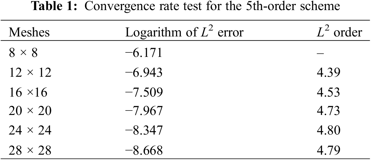
In order to test the accuracy of the present high-order scheme, we conduct the convergence rate test by solving the Euler equations with a manufactured solution. The computation domain is [0,2π]×[0,2π] with the periodic boundary conditions applied everywhere. The Euler equations are solved with the initial solution of ρ=1+0.2sin⁡θ, u=1,v=1,p=1,θ=x+y from time t = 0 to t = 0.1. The exact solution of the problem is ρ=1+0.2sin⁡θ , u=1, v=1, p=1, θ=x+y−2t . In fact, this problem is an advection problem of the density wave, which can be described by the advection equation. Still, we solve the Euler equations to examine the accuracy of the method. Here, the fifth-order scheme is chosen. The readers are also referred to [25] to find the test of the convergency rate for schemes with other orders. From the results listed in Table 1, we see that the present method gains a close convergence rate of the designed order.

3.1.2 Advection of an Entropy Wave

The initial condition for this test is defined as

(ρ,u,p)=(1+0.5e−ln⁡2⋅(x/b)2,1,1) (27)

with parameter b = 2. Under this initial condition, it becomes a linear advection problem. For instance, the work of [18] directly solved the linear advection equation for a similar test case. Here, we still solve the Euler equations. The computation is conducted on a large region of [−800, 1000] and the mesh size is h = p + 1 (p is the degree of DG solution polynomials), which is consistent with Reference [18]. The non-reflection boundary condition is adopted at two ends. Fig. 1 gives the density solutions at t = 400 for the fourth-, 5th- and 6th-order schemes. Note that the FV computations are not active in the entire computation process using the default choices on the threshold of ε2 = 1.e–4 suggested in [25]. Thus, the solutions in Fig. 1 are actually the solutions of DG methods, although Fig. 1 shows subcell solutions as mentioned above. The results obtained by directly solving the linear equation in Reference [18] are used as the reference solutions here. One can see the consistency between current results and published ones. In order to see how the FV computations affect the results, we intentionally reduce the threshold to ε2 = 1.e–6 to activate the FV computations. Now, the results computed by the 5th-order DG/FV method are displayed in Fig. 2, where the density solutions of DG and DG/FV are compared, along with the FV cells identified during the computational period. One can see that the activated FV computations have been mainly around spurious dispersive waves and eliminated oscillations while achieving comparable resolution on the smooth solution. Further test of the suggested scheme is conducted by replacing the parameter of b = 2 in Eq. (27) with b = 1.5. Similar test case is also considered in for instance [18,35]. Fig. 3 displays the results obtained by the pure DG method and the DG/FV method, both of which adopt the 5th-order DG scheme. One can see from Fig. 3 that the DG method seems to show more spurious oscillations for the case with b = 1.5 compared to the results in Fig. 1 for the case with b = 2. On the other hand, the DG/FV scheme is still able to eliminate oscillations while achieving comparable resolution on the smooth solution.

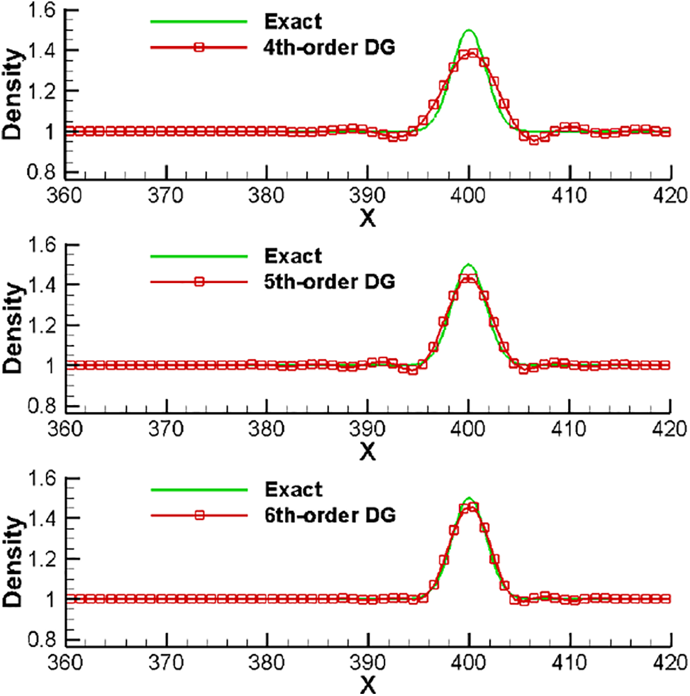
Figure 1: Comparisons between the numerical and exact solutions for advection of an entropy wave

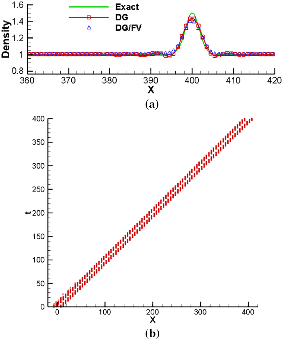
Figure 2: Density solutions obtained by the 5th-order schemes and identified FV cells for advection of an entropy wave. (a) Density solutions. (b) Identified FV cells

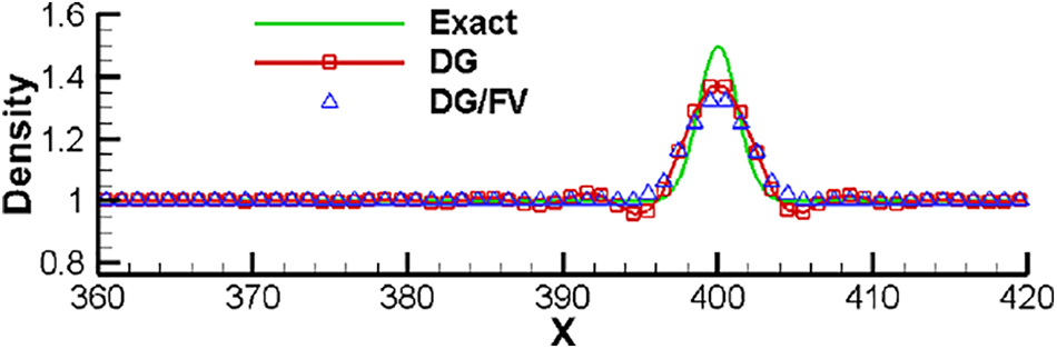
Figure 3: Comparisons between the DG and DG/FV methods using the 5th-order DG scheme for the case with b = 1.5

3.1.3 Advection of the Discontinuity

The linear advection of discontinuities is considered to test the shock-capturing property of the scheme. The computational domain is [−420, 800]. The initial conditions are

ρ=1+0.5(H(x+50)−H(x−50)),u=1,p=1. (28)

H(x) is the unit step function. The computation is performed using the 5th-order DG and DG/FV schemes on a mesh with mesh size h = 5. The density on sub-grid level at t = 200 is shown in Fig. 4, along with the FV cells identified during the computational period. We see the oscillations produced by the DG scheme have been completely eliminated by the DG/FV scheme with active FV computations mainly around the discontinuities.

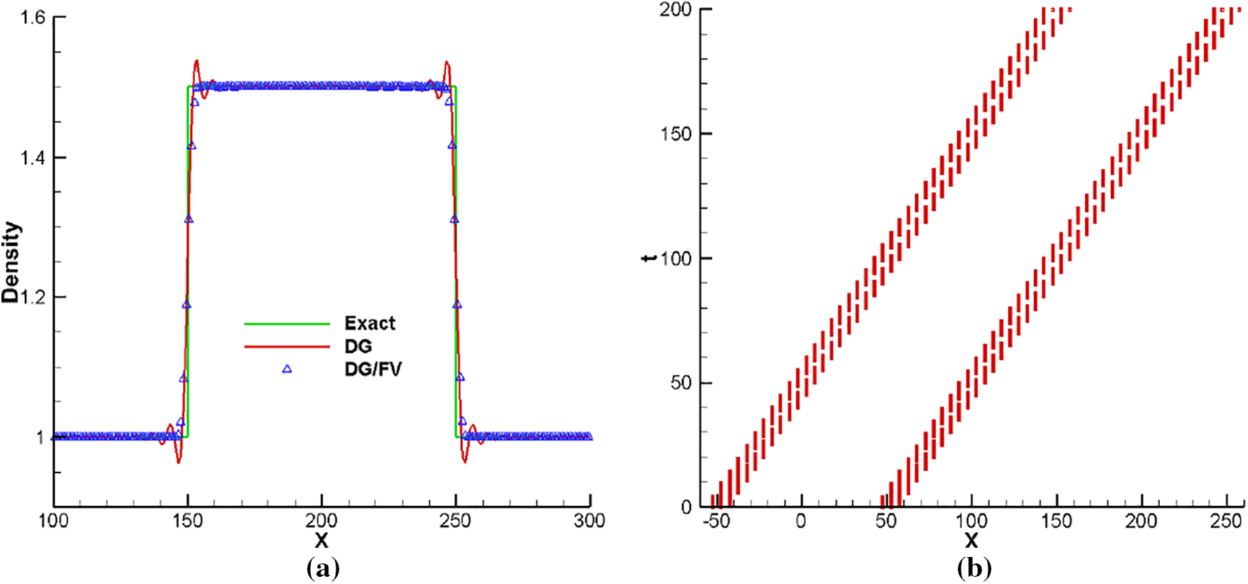
Figure 4: Density solutions obtained by the 5th-order schemes and identified FV cells for advection of the discontinuity. (a) Density solutions. (b) Identified FV cells

3.1.4 Propagation of an Acoustic Wave

The case of 1D acoustic wave propagating in a long distance is selected to verify the low dispersion and dissipation characteristics of the schemes for computational aeroacoustics. The same cases are also considered in for instance [10]. The initial conditions are set by superimposing a cosine wave to the static air with standard atmosphere pressure and room temperature. To be specific, the initial condition is given as follows:

ρ=ρ∞+ερ∞cos(2ωx),ρ∞=1.1771kg/m3u=εa∞cos(ωx)p/p∞=(ρ/ρ∞)γ,p∞=101325Paa∞=γp∞/ρ∞,γ=1.4,ω=6π,ε=10−5 (29)

Under this initial condition, an analytical solution that is derived from acoustic wave equation reads

ρ(x,t)=ρ∞+0.5ερ∞{cos[2ω(x−a∞t)]+cos[ω(x−a∞t)]+cos[2ω(x+a∞t)]−cos[ω(x+a∞t)]},u(x,t)=0.5εa∞{cos[2ω(x−a∞t)]+cos[ω(x−a∞t)]−cos[2ω(x+a∞t)]+cos[ω(x+a∞t)]},p(x,t)=p∞+0.5γεp∞{cos[2ω(x−a∞t)]+cos[ω(x−a∞t)]+cos[2ω(x+a∞t)]−cos[ω(x+a∞t)]}. (30)

The computational domain is [0, 1/3] and the periodic boundary conditions are applied at both ends. We first conduct the 6th-order scheme on a uniform mesh with 6 cells. The perturbations for density at t = 0.01 s, 0.1 s and 1 s are given in Fig. 5. We see a good agreement between the numerical and analytical solution at t = 0.01 s and 0.1 s. Slightly deviation appears after a very long propagating distance at t = 1 s. Also the solution on both main elements and subcells agrees well with the analytical one. Then, the simulation of long-time propagation to t = 1 s is carried out for the 4th order scheme using 9 cells, i.e., using the same number of DoFs as the 6th order scheme. The comparison between the two schemes is summarized in the right figure of Fig. 5. It seems that the higher-order scheme shows slightly better performance. In general, the present method in this test case demonstrates high resolution even using much coarser meshes to solve sound wave in long-distance propagation.

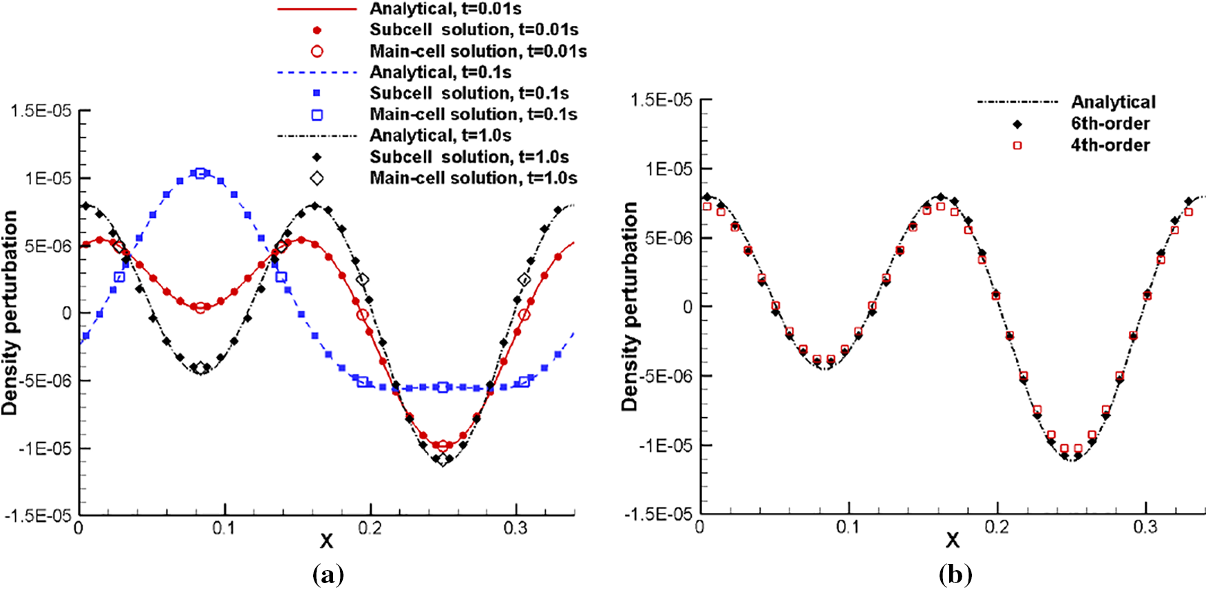
Figure 5: Density perturbation for acoustic wave propagation. (a): subcell solutions and main-cell solutions for the 6th-order scheme at different time; (b): subcell solutions for the 4th and 6th order schemes at t = 1 s obtained by using the same number of DoFs

3.1.5 Propagation of Sound, Entropy and Vorticity Waves

The test case from [2] is initially set with the an acoustic, entropy, and vorticity pulses on a uniform mean flow as

ρ=ρ∞+ε1e−a1⋅r12+ε2e−a2⋅r22,u=u∞+ε3e−a3⋅r32(y−y3),v=−ε3e−a3⋅r32(x−x3),p=p∞+ε1e−a1⋅r12 (31)

where ρ∞=1 and u∞=0.5 . The parameters include ε1=1×10−2,ε2=1×10−3,ε3=4×10−4 . al=ln⁡2/bl, l=1,2,3 with b1=3,b2=5,b3=5. rl=(x−xl)2+(y−yl)2,l=1,2,3 with (x1, y1) = (−100/3, 0), (x2, y2) = (x3, y3) = (100/3, 0). The simulation is conducted by the 6th order scheme in the zone of [−100, 100] × [−100, 100] filled with 30 × 30 grid elements. During the computation, a small number of cells have been identified as FV cells. The density perturbation counters at different time are listed in Fig. 6. Similar results are also found in for instance [11] to assess the method’s performance. Furthermore, the comparison with the reference solution [2,11] for perturbations of density and pressure along y = 0 at time t = 28.45 and t = 56.9 is plotted in Figs. 7 and 8, where both the main element solution and the subcell solution show excellent agreement with the reference one. Again, the high-order DG/FV method exhibits favorable subcell resolution on much coarser meshes.

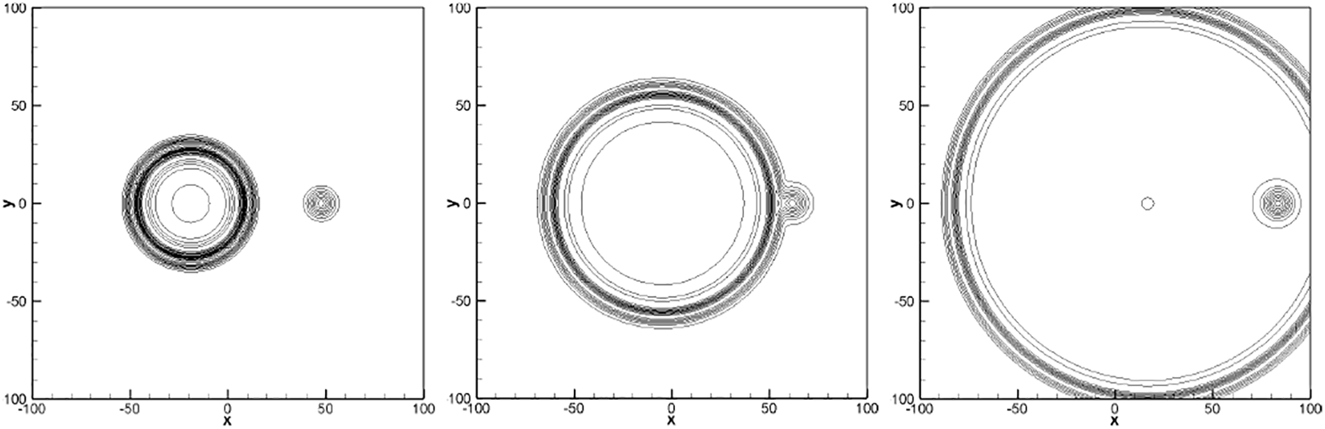
Figure 6: Contours of density perturbation for sound, entropy and vorticity waves propagation. The counters are shown in [−0.0006, 0.001] with 0.0001 increment. From left to right: t = 28.45, t = 56.9 and t = 100

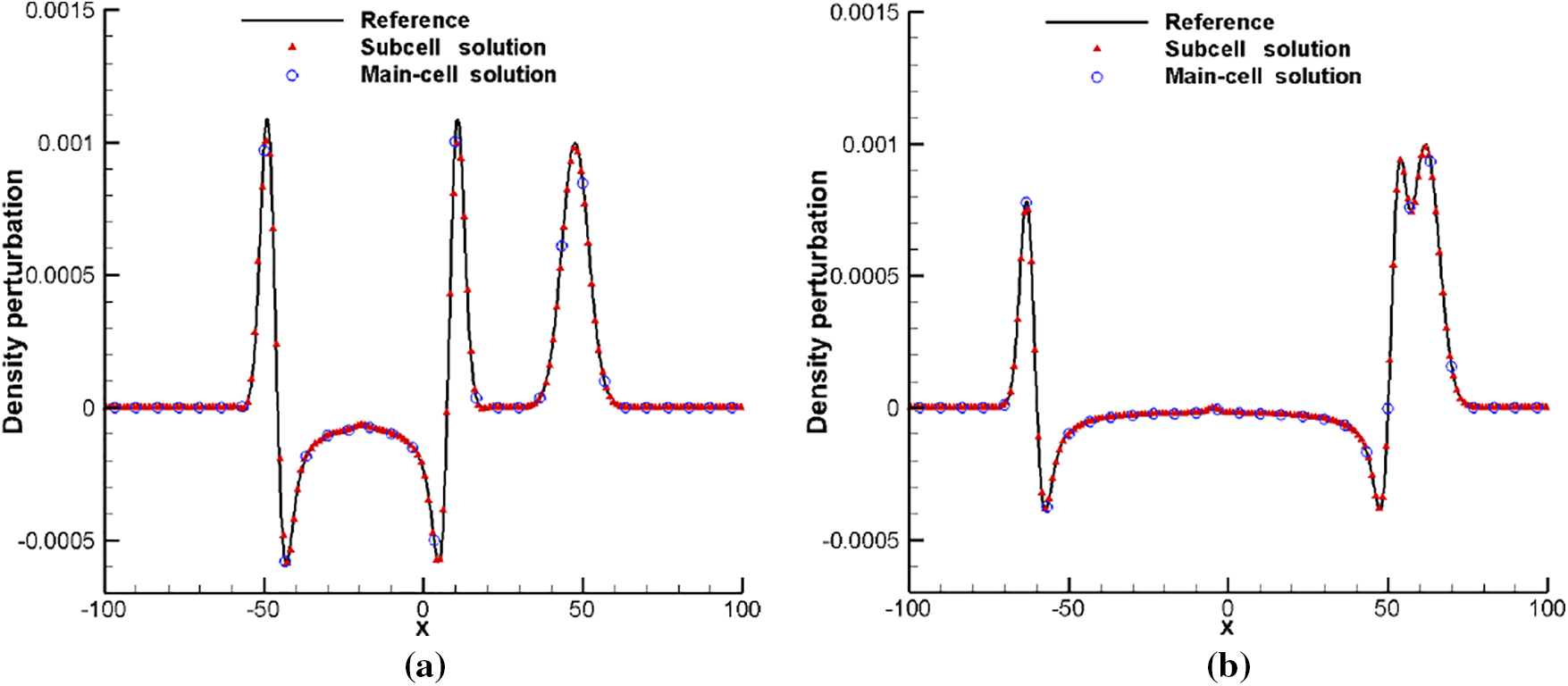
Figure 7: Perturbations of density along y = 0 for sound, entropy and vorticity waves propagation. (a) t = 28.45. (b) t = 56.9

Figure 8: Perturbations of pressure along y = 0 for sound, entropy and vorticity waves propagation. (a) t = 28.45. (b) t = 56.9

3.2 Complex Flows with Shock, Vortex and Sound Wave

In this subsection, the two-dimensional viscous flows involving shocks and vortices are considered to examine the performance of the method for simulating complex shock associated noise problems.

3.2.1 Shock Vortex Interactions

Firstly, we consider the viscous interaction of a shock wave with an isolated vortex. The computational domain is [−30,10]×[−20,20] where initially the stationary shock wave is prescribed at x = 0 while the vortex center is prescribed at (xv, yv) = (2, 0). The vortex moves from right to left with respect to the shock wave. The Mach number of the shock wave is set to be Ms = 1.2. The Reynolds number defined by Re = ρ∞a∞/μ∞ is set to be 800, and the subscript ∞ denotes the quantity in front of the shock wave. The initial vortex is given by setting tangential velocity uθ(r) = Mvre(1−r2)/2 and radial velocity ur = 0, where r=(x−xv)2+(y−yv)2 and Mv is the strength of the vortex. We use a coarse mesh with 200 × 200 points for the 6th-order DG/FV scheme. Following the representative work in such as [3,4], we first simulate the interaction at weak vortices with Mv = 0.25. The initial values of pressure and density superposed by the vortex are

p(r)=1γ[1−γ−12Mv2e(1−r2)]γ/(γ−1), ρ(r)=[1−γ−12Mv2e(1−r2)]1/(γ−1) (32)

In the computation, supersonic inflow boundary conditions are adopted at the right boundary and nonreflecting boundary conditions are given at the left boundary, while periodic boundary conditions are imposed on the top and bottom boundaries. The sound pressure is defined as Δp=(p−p∞)/p∞ , where p∞ is the pressure behind the incident shock wave.

For the interaction with weak vortices of Mv = 0.25, we compare the radial and circumferential sound pressure distributions in Fig. 9, where the results from [3] are given as the reference solution. One can see the agreement on the sound pressure is excellent between current computations and published ones.

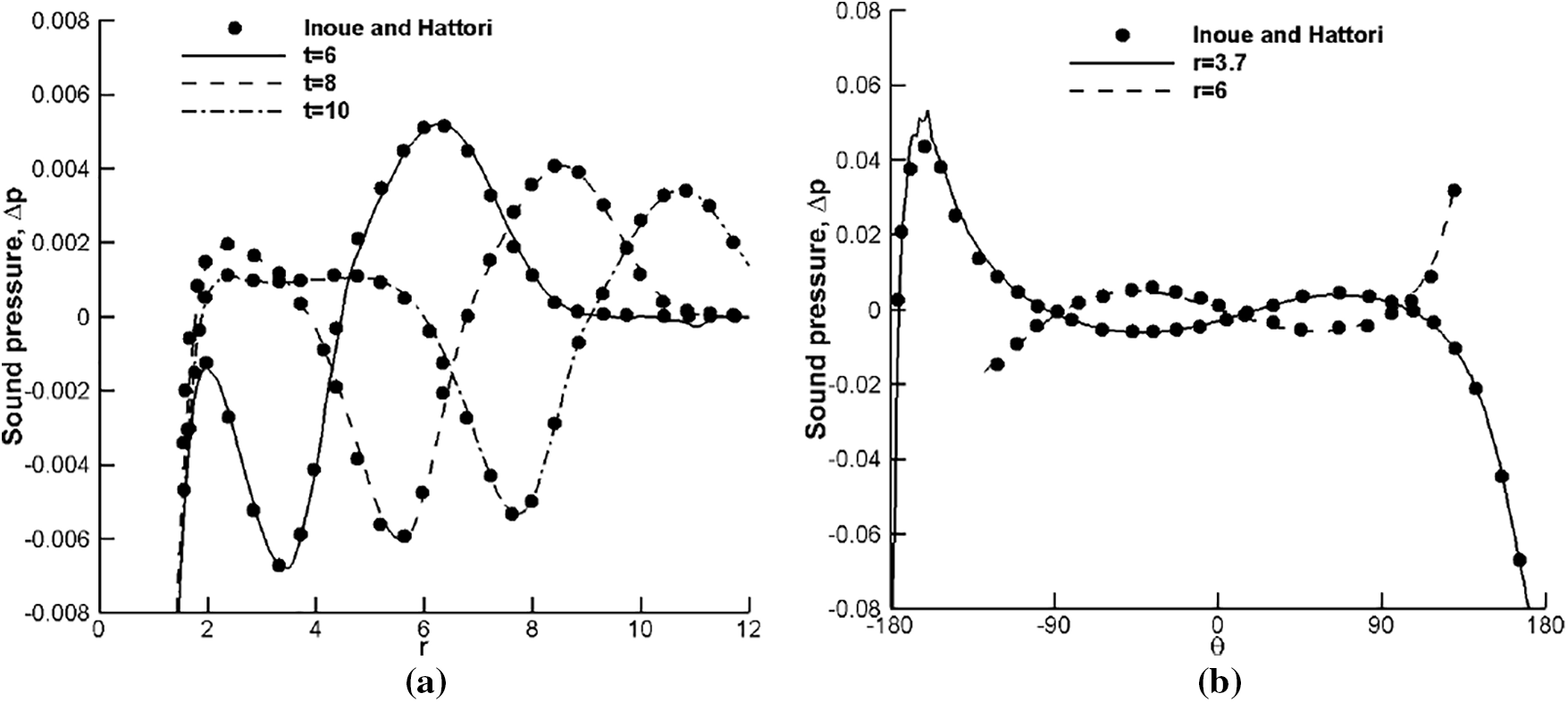
Figure 9: Radial and circumferential variations of the sound pressure against the reference solutions from [3] for shock weak-vortex interaction: Mv = 0.25, Ms = 1.2, Re = 800. (a) Radial variations at θ=−45∘ . (b) Circumferential variations at t = 6

Then we consider the interaction between a pair of vortices and a shock wave. We set the pair of vortices moves in the opposite direction as the shock wave. The case is also referred to as a collision vortex pair in [3]. The initial and boundary conditions are similarly set as the single vortex case described above. Only now the vortex center is prescribed at (xv, yv) = (2, ±2) with Mv = ±0.5 and Re = 400, which is the same as Case A for shock two-vortices interaction in [3]. In Fig. 10, we plot sound pressure counters at t = 9 and t = 13. The results show good smoothness and symmetry, supporting the high accuracy of this method. The results of Fig. 27 in [3] are also referred to as the reference solutions for the comparison.

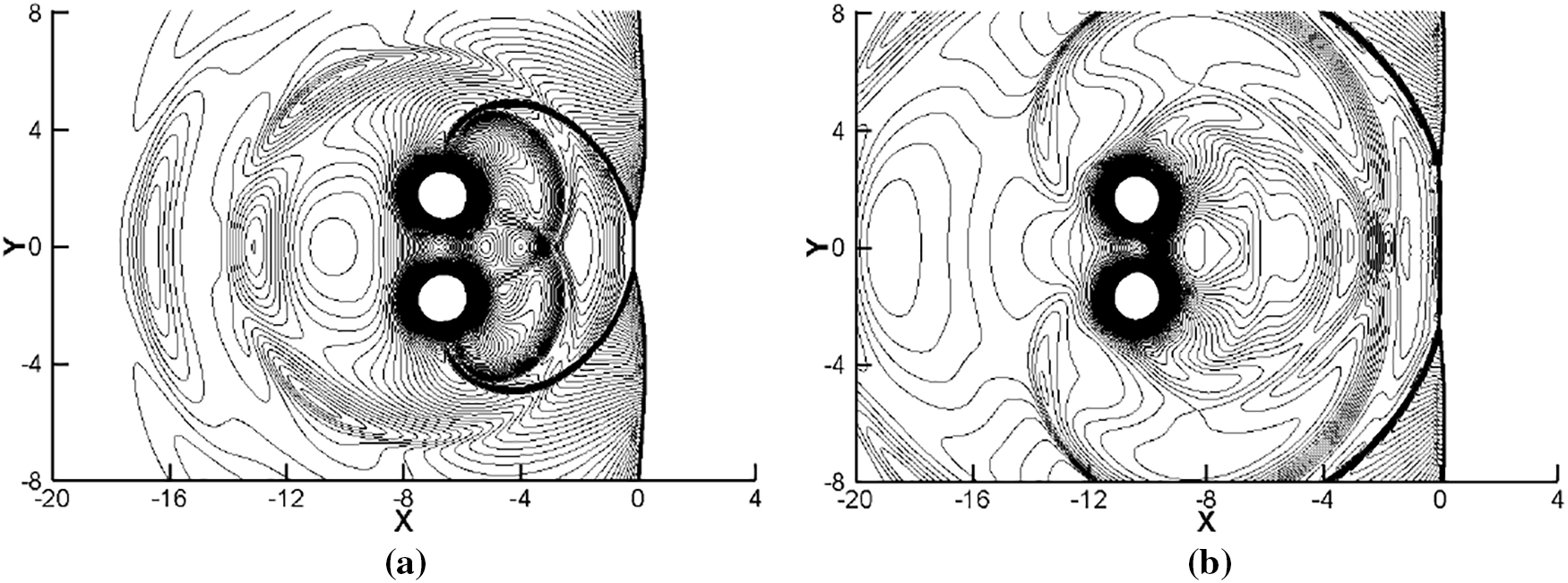
Figure 10: Sound pressure fields for shock two-vortices interaction: Mv = 0.5, Ms = 1.2, Re = 400. 80 equal-spaced counters between Δpmin=−0.2 and Δpmax=0.07 . (a) t = 9. (b) t = 13

At last, we move to the interaction of a shock wave and a strong vortex presented in [4]. Again the initial and boundary conditions are similarly set as the single vortex case but now with (xv, yv) = (4, 0) and Mv = 1.0. Fig. 11 illustrates the sound pressure contours at time t = 8, t = 12 and t = 16, where one can see the reflected shock wave extends to the vortex core region and multiple sound waves are generated due to the interactions between shocks and strong vortices. Overall, the solutions are smoothly distributed without apparent spurious oscillations. The results also agree well with previously published ones, see for instance Fig. 12 from [4]. A more quantitative comparison is similarly done in Fig. 12 by giving the radial variations of the sound pressure along the distance r from the vortex center for θ=−45∘ at t = 12 and t = 16, and by giving the circumferential variations of the sound pressure for r = 6.7, r = 12 and r = 16 at t = 16. Favorable agreement is again achieved by this computation.

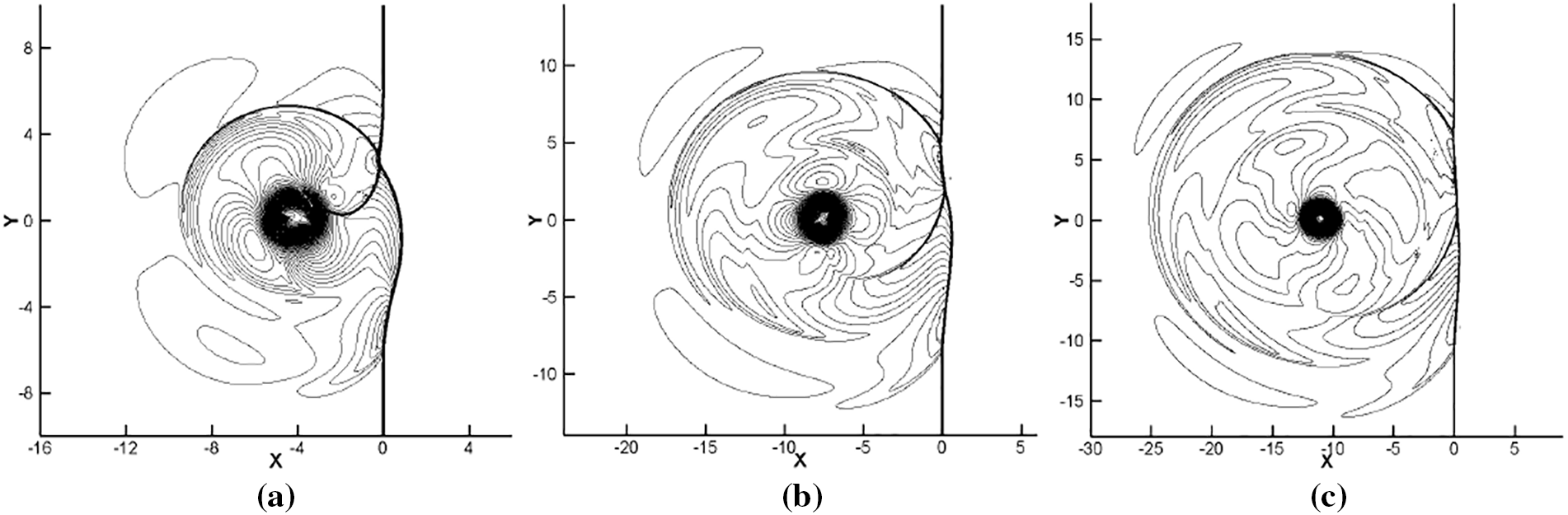
Figure 11: Sound pressure fields for shock single-vortex interaction: Mv = 1.0, Ms = 1.2, Re = 800. 80 equal-spaced counters between Δpmin=−0.9 and Δpmax=0.2 . (a) t = 8. (b) t = 12. (c) t = 16

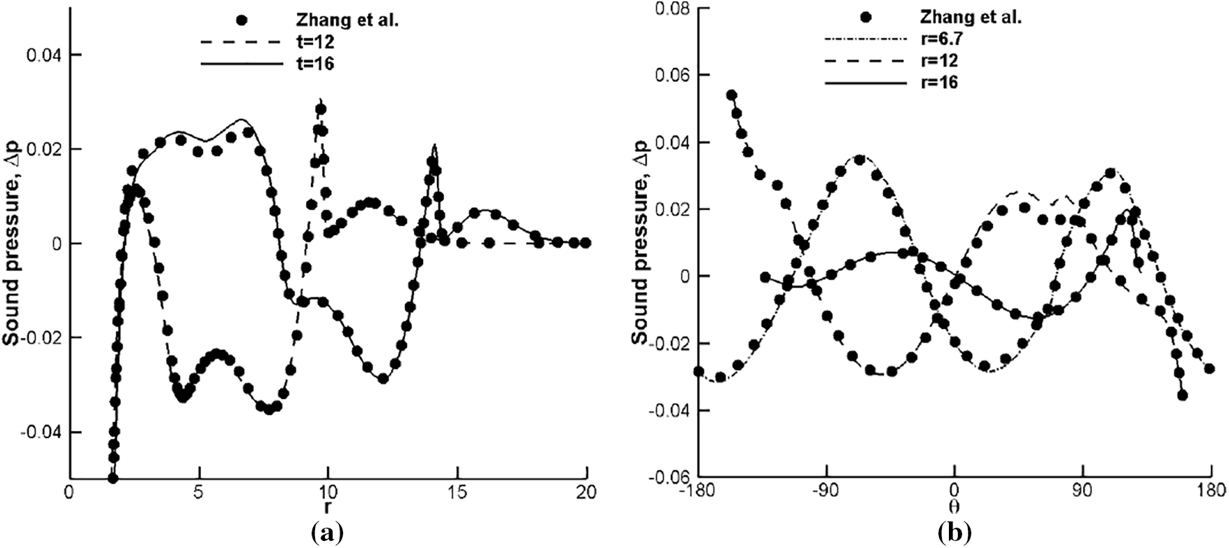
Figure 12: Radial and circumferential variations of the sound pressure against the reference solutions from [4] for shock strong-vortex interaction: Mv = 1.0, Ms = 1.2, Re = 800. (a) Radial variations at θ=−45∘ . (b) Circumferential variations at t = 16

3.2.2 Supersonic Planar Jet

A 2-D planar jet test is carried out in this subsection. The same case has been computed in for instance [11,35,36]. The flow condition is given as the jet pressure pjet = 1.4 atm, the jet Mach number Mjet = 1.4 and the jet Reynolds number Rejet = UjetL/υ = 2.8 × 105 based on the height of planar nozzle L = 0.01 m and the dynamic viscosity coefficient ν=1.73×10−5 . The computational domain is 10 L × 15 L. The entrance of the jet is located at −0.5 L ≤ y ≤ 0.5 L on the left boundary of the computational domain. Initially, the domain is filled with static gas with the specific ratio γ = 1.4, pressure p0 = 1.0 atm and temperature T0 = 300 K. The profiles of inlet flows at −0.5 L ≤ y ≤ 0.5 L are set as [37,11]

p(y)=0.5pjet[1−tanh⁡(2(|y|−L/2+2δ)/δ)],ρ(y)=0.5ρjet[1−tanh⁡(2(|y|−L/2+2δ)/δ)],u(y)=0.5Ujet[1−tanh⁡(2(|y|−L/2+2δ)/δ)], (33)

where we set δ = 4 × 10−4 m. For the rest of the left boundary the adiabatic viscous wall boundary condition is adopted, while for the upper, lower and right boundary the nonreflecting boundary condition is applied. A coarse mesh with cell edge length h ≈ 4.4 × 10−4 m is utilized in the 4th-order DG/FV computation. Fig. 13 displays the schlieren images at t = 0.08 ms, t = 0.17 ms and t = 0.24 ms, which show the development of flow structures consisting of expansion waves, shear layers, vortices and shock waves. In Fig. 13a, the precursor shock wave expands into a cylindrical form and the reflected expansion wave generates. Then, a shear layer forms and rolls up into the main vortex due to Kelvin–Helmholtz instability. The main vortex moves downstream like a mushroom head and complicated shock patterns, like shock cells, vortex-induced shock pair and embedded shocks, emerge and evolve within the flowfield. From Fig. 13b,c, we also see lots of jumps form and radiate outward. In comparison with previous results, see for instance Fig. 7 in [36], this computation seems to obtain more unstable trailing shear layers. As a result, the earlier rolling up of vortexlets and more complicated shock patterns appear. One can also see results in [11] for more refined simulation for this case. To characterize the geometry of main vortex, some geometric parameters are defined, including the distances from the nozzle entrance to the main vortex front interface and its core along x direction and the distance between two main vortex cores. These geometric parameters at t = 0.08 ms, t = 0.17 ms and t = 0.24 ms are given in Fig. 14, where the reference solutions from [36] are displayed as well. Overall, the computed geometric parameters agree well with the reference, except that the distance between the entrance and the vortex core, denoted by Xv, seems to be slightly larger. We mention the 2-D computation in [36] also exhibited certain vibrations for the prediction of Xv and Dm. Generally speaking, in this challenging case for the high order method, the DG/FV method is capable of capturing discontinuities with sharp transition while resolving delicate vortex structures on the coarse mesh.

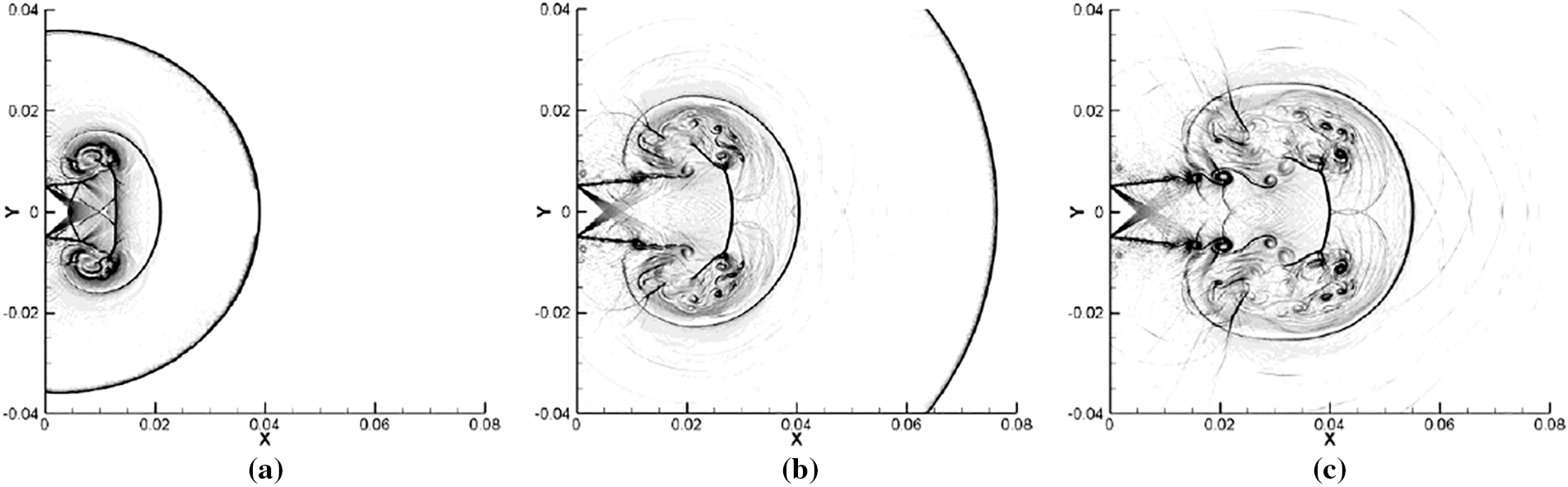
Figure 13: Numerical schlieren images for supersonic planar jet at different time. (a) t = 0.08 ms. (b) t = 0.17 ms. (c) t = 0.24 ms

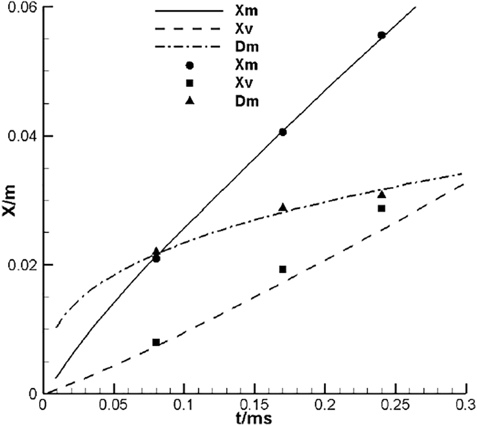
Figure 14: The position of vortex front (Xm) and core (Xv) along x direction and the core diameter (Dm) at t = 0.08 ms, 0.17 ms and 0.24 ms. The reference results from [36] are indicated with lines while the computed results are indicated with symbols

3.2.3 Shock Shear-Layer Interactions

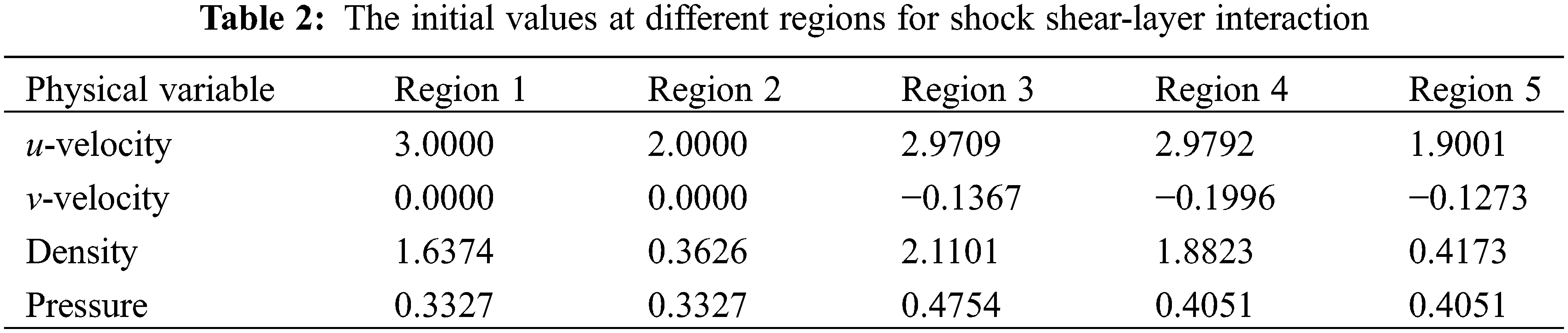
The interaction of a shock wave and a shear-layer contains complex flow structures such as vortices arising from the shear layer instability as well as their interacting with the shock system. Thus it provides a good test case to examine the performance of numerical schemes. Here, we select the case of shock shear-layer interaction from [38]. The computation domain is a rectangle of [0, 200] × [−20, 20]. The initial states for five different regions illustrated in Fig. 15 are set up with values listed in Table 2. The Reynolds number is chosen to be 500. The upper boundary is given the flow properties behind the oblique shock, which are thus the same values for Region 3 in Table 2. The lower boundary is specified with the slip condition. The outflow boundary condition is set for the right boundary, while the inflow is specified with a hyperbolic tangent profile. This profile gives a mixing layer with the upper velocity equal to 3 and the lower velocity equal to 2. Moreover, the fluctuations are added to the inflow velocity, see [38] for more details about the inflow profile and the fluctuations.

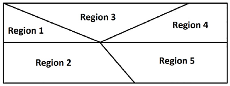
Figure 15: Illustration of different regions in flowfield initialization for shock shear-layer interaction

The test case has been run using the 6th-order scheme on a coarse grid with 240 × 60 elements. A typical flowfield at t = 120 is given in Fig. 16 by showing the dilatation contour and the density solutions, along with the identified FV cells at the same time. We see the oblique shock impacts on the shear layer at around x = 90. The impact causes the change of the shock angle as well as the deflection of the shear layer. The shock wave below the shear layer reflects from the lower boundary and again passes through the shear layer at around x = 140. There exist strong compression and expansion waves in the flowfield. At the region of x > 150 several eddy shock waves starts to form around the vortices. Complex interactions between the transmitted shocks, the eddy shocks and the vortices are seen in the region. Overall, the results obtained by this computation are comparable to the published ones, see for instance Fig. 4 in [38] for the reference of density results and Fig. 12 in [39] for the reference of dilatation results. The dilatation solutions in the sub-grid level seem to be slightly oscillatory. Another interesting observation is that the FV computation is not activated at the beginning of the shear layer until the mixing layer starts to lose the stability, see the identified FV cells at the same time in Fig. 16. As for the small oscillations in the sub-grid level, they do not affect the general high accuracy of the method. To demonstrate this point, we give a more quantitative comparison through the density field between x = 50 and x = 150 at y = 0. The reference solution is again from [38], which is obtained by performing high order finite difference scheme on much refined meshes. From Fig. 17, the present method has achieved almost identical agreement against the reference solution, indicating the desirable performance of the high-order DG/FV method in using the coarser meshes to simulate such complex flows.

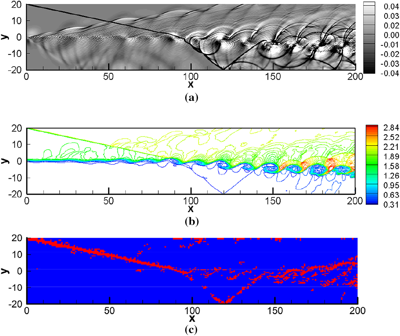
Figure 16: The flowfield results at t = 120 for shock shear-layer interaction. (a) The dilatation contour. (b) The density counter. (c) The FV cells indicated with red color

Figure 17: The distribution of density along y = 0 at t = 120 against the reference solution from [38] for shock shear-layer interaction

4  Conclusion

In this work, we have suggested the high-order DG/FV method for computational aeroacoustics and tested the performance of the method for shocked-associated noise problems. The high-order DG/FV method achieves subcell resolution and low dissipation properties, which play an important role in simulating aeroacoustic problems. The high-fidelity discontinuity-capturing scheme under the BVD reconstruction paradigm shows desirable features in terms of eliminating spurious oscillations and maintaining high resolution on both the discontinuities and the smooth flow structures. In particular, the method of using higher-order schemes shows the favorable characteristic through the use of coarse meshes to gain comparable and even better resolution for the smooth acoustic wave. The superiority of the proposed method on the coarse meshes is more related to the high resolution of the high-order DG scheme, which results from having more degrees of freedom. Numerical tests on complex flows involving strong shock-vortex interactions also reveal that the method is able to capture various discontinuities without generating spurious oscillations and maintain the high resolution on smooth and delicate flow structures. Good agreement on the sound pressure and density solution in quantitative comparison with the finite difference or finite volume scheme also indicates the superior performance of the high-order DG/FV method.

Acknowledgement: None.

Funding Statement: The research was supported by the National Natural Science Foundation of China under Grant Nos. 92252201 and 11721202. The research was also support by the Laboratory of Aerodynamic Noise Control under Grant No. 2301ANCL20230303 and the Fundamental Research Funds for the Central Universities.

Author Contributions: The authors confirm contribution to the paper as follows: study conception and design: Zhenhua Jiang, Xi Deng, Chao Yan, Feng Xiao; data collection: Zhenhua Jiang, Xin Zhang; analysis and interpretation of results: Zhenhua Jiang, Jian Yu; draft manuscript preparation: Zhenhua Jiang, Xi Deng. All authors reviewed the results and approved the final version of the manuscript.

Availability of Data and Materials: The data that support the findings of this study are available from the corresponding author upon reasonable request.

Ethics Approval: Not applicable.

Conflicts of Interest: The authors declare that they have no conflicts of interest to report regarding the present study.

References

1. Lele SK. Compact finite difference schemes with spectral-like resolution. J Comput Phys. 1992;103(1):16–42. doi:10.1016/0021-9991(92)90324-R. [Google Scholar] [CrossRef]

2. Tam CKW, Webb JC. Dispersion-relation-preserving finite difference schemes for computational acoustics. J Comput Phys. 1993;107(2):262–81. doi:10.1006/jcph.1993.1142. [Google Scholar] [CrossRef]

3. Inoue O, Hattori Y. Sound generation by shock-vortex interactions. J Fluid Mech. 1999;380:81–116. doi:10.1017/S0022112098003565. [Google Scholar] [CrossRef]

4. Zhang S, Zhang YT, Shu C-W. Multistage interaction of a shock wave and a strong vortex. Phys Fluids. 2005;17(11):116101. doi:10.1063/1.2084233. [Google Scholar] [CrossRef]

5. Adams NA, Shariff K. A high-resolution hybrid compact-ENO scheme for shock-turbulence interaction problems. J Comput Phys. 1996;127(1):27–46. doi:10.1006/jcph.1996.0156. [Google Scholar] [CrossRef]

6. Deng X, Zhang H. Developing high-order weighted compact nonlinear schemes. J Comput Phys. 2000;165(1):22–44. doi:10.1006/jcph.2000.6594. [Google Scholar] [CrossRef]

7. Wang Z, Chen R. Optimized weighted essentially nonoscillatory schemes for linear waves with discontinuity. J Comput Phys. 2001;174(1):381–404. doi:10.1006/jcph.2001.6918. [Google Scholar] [CrossRef]

8. Popescu M, Shyy W, Garbey M. Finite volume treatment of dispersion-relation-preserving and optimized prefactored compact schemes for wave propagation. J Comput Phys. 2005;210(2):705–29. doi:10.1016/j.jcp.2005.05.011. [Google Scholar] [CrossRef]

9. Daru V, Gloerfelt X. Aeroacoustic computations using a high-order shock-capturing scheme. AIAA J. 2007;45(10):2474–86. doi:10.2514/1.28518. [Google Scholar] [CrossRef]

10. Bai Z, Zhong X. New very high-order upwind multi-layer compact (MLC) schemes with spectral-like resolution for flow simulations. J Comput Phys. 2019;378:63–109. doi:10.1016/j.jcp.2018.10.049. [Google Scholar] [CrossRef]

11. Zhao F, Ji X, Shyy W, Xu K. An acoustic and shock wave capturing compact high-order gas-kinetic scheme with spectral-like resolution. Int J Comput Fluid Dyn. 2020;34(10):731–56. [Google Scholar]

12. Cockburn B, Shu C-W. The Runge-Kutta discontinuous Galerkin method for conservation laws V: multidimensional systems. J Comput Phys. 1998;141:199–224. [Google Scholar]

13. Hu FQ, Hussaini MY, Rasetarinera P. An analysis of the discontinuous Galerkin method for wave propagation problems. J Comput Phys. 1999;151(2):921–46. [Google Scholar]

14. Sherwin S. Dispersion analysis of the continuous and discontinuous Galerkin formulations. In: Discontinuous Galerkin methods. Berlin: Springer; 2000. p. 425–31. doi:10.1007/978-3-642-59721-3_43. [Google Scholar] [CrossRef]

15. Ainsworth M. Dispersive and dissipative behaviour of high order discontinuous Galerkin finite element methods. J Comput Phys. 2004;198(1):106–30. [Google Scholar]

16. Zhong X, Shu C-W. Numerical resolution of discontinuous Galerkin methods for time dependent wave equations. Comput Methods Appl Mech Eng. 2011;200:2814–27. [Google Scholar]

17. Guo W, Zhong X, Qiu JM. Superconvergence of discontinuous Galerkin and local discontinuous Galerkin methods: eigen-structure analysis based on Fourier approach. J Comput Phys. 2013;235:458–85. doi:10.1016/j.jcp.2012.10.020. [Google Scholar] [CrossRef]

18. Cheng Z, Fang J, Shu C-W, Zhang M. Assessment of aeroacoustic resolution properties of DG schemes and comparison with DRP schemes. J Comput Phys. 2019;399(1):108960. doi:10.1016/j.jcp.2019.108960. [Google Scholar] [CrossRef]

19. Fechter S, Hindenlang F, Frank H, Munz CD, Gassner G. Discontinuous Galerkin schemes for the direct numerical simulation of fluid flow and acoustics. In: 18th AIAA/CEAS Aeroacoustics Conference (33rd AIAA Aeroacoustics Conference), 2012; Colorado Springs, CO, USA. doi:10.2514/6.2012-2187. [Google Scholar] [CrossRef]

20. Shi J, Yan H, Wang ZJ. Towards direct computation of aeroacoustic noise with the high-order FR/CPR method. In: 2018 AIAA/CEAS Aeroacoustics Conference, 2018; Atlanta, GA, USA. doi:10.2514/6.2018-4095. [Google Scholar] [CrossRef]

21. Lorteau M, de la Llave Plata M, Couaillier V. Turbulent jet simulation using high-order DG methods for aeroacoustic analysis. Int J Heat Fluid Flow. 2018;70(5):380–90. doi:10.1016/j.ijheatfluidflow.2018.01.012. [Google Scholar] [CrossRef]

22. Shen W, Miller SAE. Validation of a high-order large eddy simulation solver for acoustic prediction of supersonic jet flow. J Theor Comput Acoust. 2020;28(3):1950023. doi:10.1142/S2591728519500233. [Google Scholar] [CrossRef]

23. Colombo A, Crivellini A, Ghidoni A, Nigro A, Noventa G. An implicit p-adaptive discontinuous Galerkin solver for CAA/CFD simulations. Int J Numer Methods Fluids. 2022;94(8):1269–97. doi:10.1002/fld.5089. [Google Scholar] [CrossRef]

24. Deng X, Jiang Z, Xiao F, Yan C. Implicit large eddy simulation of compressible turbulence flow with PnTm-BVD scheme. Appl Math Model. 2020;77(4):17–31. doi:10.1016/j.apm.2019.07.022. [Google Scholar] [CrossRef]

25. Jiang Z, Deng X, Xiao F, Yan C, Yu J, Lou S. Hybrid discontinuous Galerkin/finite volume method with subcell resolution for shocked flows. AIAA J. 2021;59(6):2027–44. doi:10.2514/1.J059763. [Google Scholar] [CrossRef]

26. Bassi F, Crivellini A, Rebay S, Savini M. Disontinuous Galerkin solution of the Reynolds-averaged Navier-Stokes and k-ω turbulence model equations. Comput Fluids. 2005;34(4–5):507–40. doi:10.1016/j.compfluid.2003.08.004. [Google Scholar] [CrossRef]

27. Huerta A, Casoni E, Peraire J. A simple shock-capturing technique for high-order discontinuous Galerkin methods. Int J Numer Methods Fluids. 2012;69(10):1614–32. doi:10.1002/fld.2654. [Google Scholar] [CrossRef]

28. Sonntag M, Munz CD. Shock capturing for discontinuous Galerkin methods using finite volume subcells. In: Fuhrmann J, Ohlberger M, Rohde C, editors. Finite volumes for complex applications VII. Cham: Springer; 2014. p. 945–53. doi:10.1007/978-3-319-05591-6_96. [Google Scholar] [CrossRef]

29. Dumbser M, Zanotti O, Loubère R, Diot S. A posteriori subcell limiting of the discontinuous Galerkin finite element method for hyperbolic conservation laws. J Comput Phys. 2014;278:47–75. [Google Scholar]

30. Vilar F. A posteriori correction of high-order discontinuous Galerkin scheme through subcell finite volume formulation and flux reconstruction. J Comput Phys. 2019;387:245–79. [Google Scholar]

31. Persson PO, Stamm B. A discontinuous Galerkin method for shock capturing using a mixed high-order and sub-grid low-order approximation space. J Comput Phys. 2022;449:110765. [Google Scholar]

32. Sun Z, Inaba S, Xiao F. Boundary variation diminishing (BVD) reconstruction: a new approach to improve Godunov schemes. J Comput Phys. 2016;322:309–25. [Google Scholar]

33. Xiao F, Honma Y, Kono T. A simple algebraic interface capturing scheme using hyperbolic tangent function. Int J Numer Methods Fluids. 2005;48(9):1023–40. [Google Scholar]

34. Deng X, Jiang Z, Vincent P, Xiao F, Yan C. A new paradigm of dissipation-adjustable, multi-scale resolving schemes for compressible flows. J Comput Phys. 2022;466(1):111287. doi:10.1016/j.jcp.2022.111287. [Google Scholar] [CrossRef]

35. Zhao F, Ji X, Shyy W, Xu K. Direct modeling for computational fluid dynamics and the construction of high-order compact scheme for compressible flow simulations. J Comput Phys. 2023;477(1):111921. doi:10.1016/j.jcp.2023.111921. [Google Scholar] [CrossRef]

36. Zhang H, Chen Z, Jiang X, Huang Z. The starting flow structures and evolution of a supersonic planar jet. Comput Fluids. 2015;114:98–109. doi:10.1016/j.compfluid.2015.02.013. [Google Scholar] [CrossRef]

37. Zhao W, Frankel SH, Mongeau LG. Effects of trailing jet instability on vortex ring formation. Phys Fluids. 2000;12(3):589–96. doi:10.1063/1.870264. [Google Scholar] [CrossRef]

38. Sandham ND, Yee HC. Performance of low dissipative high order shock-capturing schemes for shock-turbulence interactions. NASA Ames Research Center; 1998. RIACS Technical Report 98.10. [Google Scholar]

39. Liu X, Zhang S. Direct numerical simulation of the interaction of 2D shock wave and shear layer. Chin J Theor Appl Mech. 2013;45:61–75 (In Chinese). [Google Scholar]