
 Submit a Paper
 Propose a Special lssue
 Open Access
ARTICLE

Evaluation and Application of Flowback Effect in Deep Shale Gas Wells
Shale Gas Research Institute, PetroChina Southwest Oil & Gas field Company, Chengdu, 610051, China
* Corresponding Author: Sha Liu. Email:
(This article belongs to the Special Issue: Fluid and Thermal Dynamics in the Development of Unconventional Resources II)
Fluid Dynamics & Materials Processing 2024, 20(10), 2301-2321. https://doi.org/10.32604/fdmp.2024.052454
Received 02 April 2024; Accepted 06 June 2024; Issue published 23 September 2024
 View Full Text
 Download PDF
Abstract
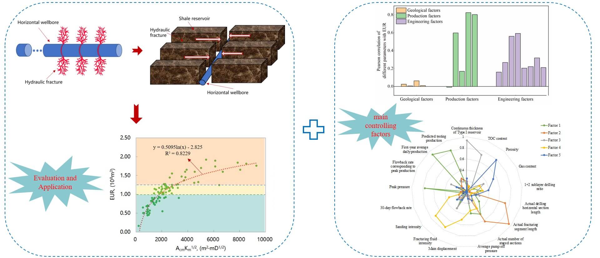
The pivotal areas for the extensive and effective exploitation of shale gas in the Southern Sichuan Basin have recently transitioned from mid-deep layers to deep layers. Given challenges such as intricate data analysis, absence of effective assessment methodologies, real-time control strategies, and scarce knowledge of the factors influencing deep gas wells in the so-called flowback stage, a comprehensive study was undertaken on over 160 deep gas wells in Luzhou block utilizing linear flow models and advanced big data analytics techniques. The research results show that: (1) The flowback stage of a deep gas well presents the characteristics of late gas channeling, high flowback rate after gas channeling, low 30-day flowback rate, and high flowback rate corresponding to peak production; (2) The comprehensive parameter AcmKm1/2 in the flowback stage exhibits a strong correlation with the Estimated Ultimate Recovery (EUR), allowing for the establishment of a standardized chart to evaluate EUR classification in typical shale gas wells during this stage. This enables quantitative assessment of gas well EUR, providing valuable insights into production potential and performance; (3) The spacing range and the initial productivity of gas wells have a significant impact on the overall effectiveness of gas wells. Therefore, it is crucial to further explore rational well patterns and spacing, as well as optimize initial drainage and production technical strategies in order to improve their performance.Graphic Abstract
Keywords
Nomenclature
| | Dimensionless production |
| | Dimensionless time, |
| | Area of gas flow from the matrix to the fracture, that is, the contact area between the matrix and the fracture, m2 |
| | Matrix permeability of shale gas reservoir, mD |
| | Formation temperature, ℉ |
| | Formation porosity, fraction |
| | Gas viscosity, mPa·s |
| | Comprehensive gas compressibility coefficient, MPa−1 |
| | Original formation pressure, MPa |
| | Bottom hole flowing pressure of gas well, MPa |
| | Gas pseudo-pressure, MPa2/(mPa·s) |
| | Slope of the linear flow stage in RNP and t1/2 curve, dimensionless |
| | Equivalent total surface flow rate, m3/h |
| | Instantaneous gas production rate at the shale gas wellhead, m3/h |
| | Instantaneous water production rate at the shale gas wellhead, m3/h |
| | Dimensionless gas volume coefficient, fraction |
| | Dimensionless water volume coefficient, fraction |
Shale gas reservoirs are typical “artificial gas reservoirs”. In order to achieve large-scale and efficient development, a combination of “horizontal wells + volume fracturing technology” is necessary. Currently, the shale gas production in the Southern Sichuan Basin mainly relies on the volume fracturing scale of “ten thousand cubic meters of liquid + thousand cubic meters of sand” [1], with more than a thousand wells in production. The success of large-scale development will directly impact the realization of increasing reserves and production of shale gas, as well as the extent to which natural gas demand can be met [2,3]. In 2022, shale gas production in the Southern Sichuan Basin reached 139.2 × 10⁸ m3, representing an increase of 10.5 × 10⁸ m3 compared with that in 2021, indicating a year-on-year growth of 8.2%. This has laid the foundation for the large-scale and efficient development of shale gas in the southern Sichuan Basin. In this region, the primary focus is on the efficient and stable production of mid-deep gas wells (depth less than 3500 m) and the large-scale increase in production of deep gas wells (depth ranging from 3500 to 4500 m). Efforts are concentrated on enhancing the performance of individual wells and vigorously promoting productivity construction. As of January 2024, more than 180 deep shale gas wells have been put into operation in the Luzhou block, with a daily gas production exceeding 600 × 104 m3 (Fig. 1).
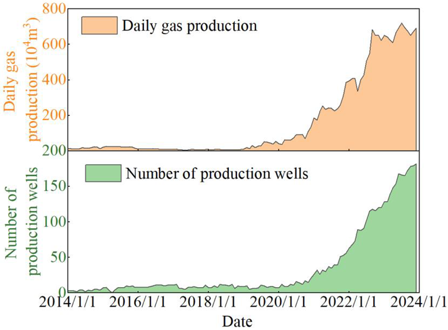
Figure 1: Production status of deep shale gas wells in the Luzhou block
Currently, the post-fracturing flowback of shale gas wells in the southern Sichuan Basin is being conducted by progressively enlarging the choke. This process not only helps clear pathways for gas infiltration but also serves as a crucial stage for evaluating the post-fracturing effects of gas wells and maximizing the retention of reservoir energy. However, due to the more complex geological and engineering conditions of deep shale gas wells, there is still a limited understanding of the characteristics and patterns of the flowback stage. Additionally, a systematic evaluation method and process for assessing the effectiveness of the gas wells in the flowback stage have not been established. As a result, accurately predicting the Estimated Ultimate Recovery (EUR) of gas wells during flowback stage remains challenging. The data samples for the deep shale gas wells in flowback stage are extensive, so how to effectively extract key information and conduct research analysis is essential for evaluating the flowback effects and guiding the productivity maintenance of gas wells in the later stages.
In recent years, various methods have been employed to evaluate the flowback effects of gas wells, including analytical models, numerical simulation, artificial intelligence, big data analysis, and data-driven approaches [4–7]. Some scholars have also integrated numerical simulation with machine learning methods to improve the adaptability and reliability of models [8–10]. However, due to the complex effects of fracture propagation and fracture network after fracturing [11,12], as well as the large liquid volumes in the early flowback stage and the intricate flow patterns of gas and liquid in the wellbore [13,14], analytical models and numerical simulation methods impose strict requirements on basic parameters and exhibit limited adaptability in practical gas well analysis, resulting in the inability to predict EUR during the early flowback stage in a timely manner. In addition, data-driven approaches based on artificial intelligence and big data analysis, are capable of quickly obtaining characteristic information during the flowback stage. Nevertheless, they still encounter challenges such as high sample analysis demands and difficulty in filtering out abnormal information which can affect model precision.
Based on the characteristics and the flow patterns of shale gas well in the early flowback stage, this article has established a method for rapidly evaluating the flowback effects. This method allows for the establishment of a classification evaluation chart of deep gas well effects in the Luzhou block, as well as timely and accurate prediction of gas well EUR. Furthermore, it provides a foundational guarantee for rational production allocation, production system optimization, and well pattern deployment optimization (i.e., optimization of development technology strategy). Specially, through the integration of geological, engineering, and production characteristic factors, as well as the utilization of anomaly data screening and big data analysis methods, a comprehensive analysis was conducted to identify the main controlling factors influencing the performance of gas wells, focusing on continuously improving individual well production in order to support the large-scale and efficient development of deep shale gas.
2 Characteristics of Deep Shale Gas Wells in the Luzhou Block
2.1 Geological Engineering Characteristics
The marine shales in the Ordovician Wufeng Formation and the Silurian Longmaxi Formation in the Sichuan Basin exhibit superior quality and are currently the primary focus of shale gas exploration and development. After more than a decade of exploration, commercial and large-scale development of shale gas in the mid-deep layers has been achieved [15]. Additionally, the favorable working area for deep layers with burial depths ranging from 3500 to 4500 m covers an area of 1.2 × 10⁴ km2, with geological resource volume amounts to 6.6 × 10¹² m3, which is a key target for achieving the goals of “Gas Daqing” and “Dual Carbon” initiative [16].
The engineering characteristic factors of deep shale gas reservoirs in China generally exhibit the “Five Highs”: high Poisson’s ratio and elastic modulus, high formation temperature, high horizontal stress difference, high fracturing initiation pressure, and high closure pressure [17]. Additionally, deep shale gas reservoirs are characterized by deeper burial, higher temperature, and more complex geological conditions, posing significant challenges in well drilling engineering, well completion engineering, and development [18]. These challenges manifest in seven main aspects: ① More challenging drilling orientation; ② Higher formation temperature (>120°C); ③ Higher formation pressure (>80 MPa); ④ Larger horizontal stress difference (15–25 MPa) and higher closure stress (90–100 MPa); ⑤ Higher exploration and development costs; ⑥ Unclear development technology strategies; ⑦ Unresolved multi-scale gas flow patterns.
2.2 Flowback Characteristics of Deep Shale Gas Wells
Before a shale gas well officially enters production, it undergoes the flowback stage, which typically lasts from 1 to 4 months. Deep shale gas wells generally exhibit characteristics such as a late onset of gas breakthrough, high flowback rate, low initial production, rapid production decline, and a long production cycle [19]. Due to factors such as frequent adjustments of gas well choke, inter-well fracturing channeling, wellbore liquid loading, sand plugging and workovers, the wellhead pressure, gas production rate and liquid production rate exhibit significant fluctuations over time, showing poor overall regularity. The whole life cycle of deep shale gas wells from flowback to official production can be divided into three stages, namely, the well soaking stage, the flowback stage, and the production stage. Based on the changing patterns of gas production rate, liquid production rate and wellhead pressure, the flowback stage of typical deep shale gas wells can be further subdivided into three smaller stages (Fig. 2):
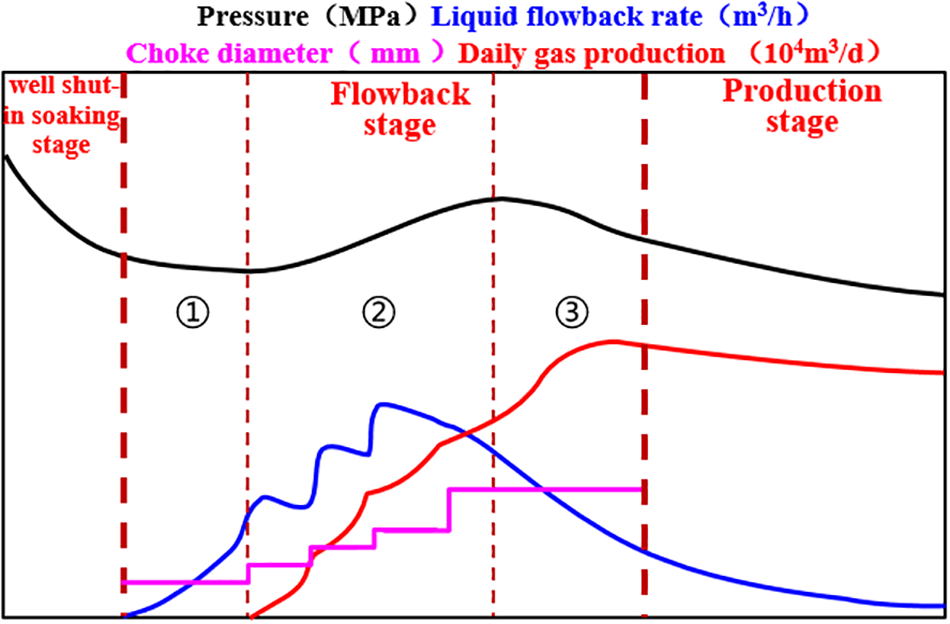
Figure 2: Typical flowback curves of shale gas well
Flowback stage ①: Well opening without gas channeling. Liquid production rate continues to rise, and wellhead casing pressure initially decreases and then increases.
Flowback stage ②: Liquid production rate, gas production rate and wellhead pressure increase simultaneously, and wellhead pressure reaches its peak. Due to the wellbore unloading effect, the wellhead pressure usually gradually rises after gas channeling until it reaches its peak.
Flowback stage ③: Wellhead pressure and liquid production rate decrease, and gas production rate gradually decreases after reaching its peak.
Fig. 3 illustrates the curve of an actual deep shale gas well of the flowback stage in the Luzhou block, corresponding to the three stages in the typical flowback curve.
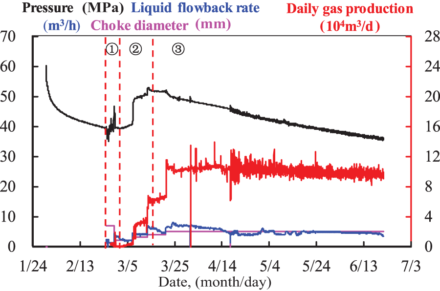
Figure 3: Flowback of a shale gas well in the Luzhou block
Currently, four major flowback evaluation indicators have been established for shale gas wells in the mid-deep layers in the Southern Sichuan Basin: gas channeling time, gas channeling flowback rate, 30-day flowback rate, and flowback rate corresponding to peak production. However, these indicators are not adaptable to deep gas wells, making it challenging to accurately assess their performance (Fig. 4). When compared with mid-deep shale gas wells in the Sichuan Basin (Changning block), deep shale gas wells (Luzhou block and Yuxi block) exhibit characteristics such as later gas channeling, higher gas channeling flowback rate, lower 30-day flowback rate, and higher flowback rate corresponding to peak production (Fig. 5).
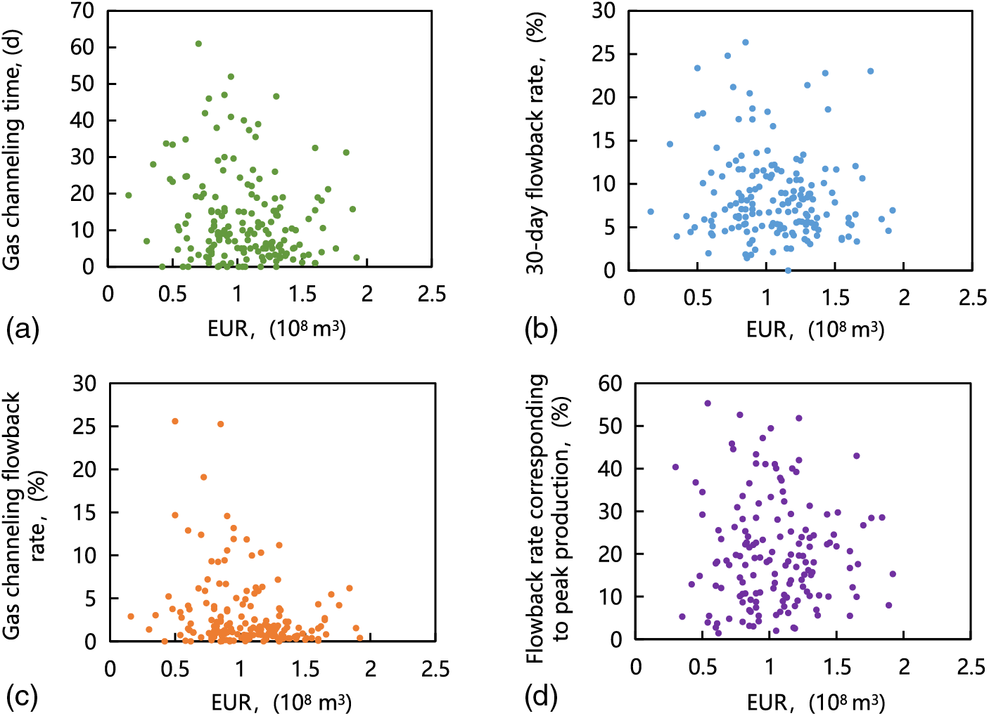
Figure 4: Distribution of early flowback indicators of deep gas wells (a) Gas channeling time and EUR distribution; (b) Gas channeling flowback rate and EUR distribution; (c) 30-day flowback rate and EUR distribution; (d) Flowback rate corresponding to peak production and EUR distribution
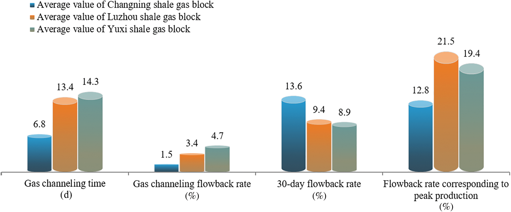
Figure 5: Comparison of flowback indicators between mid-deep gas wells and deep gas wells
3 Effect Evaluation of Flowback Stage
Due to the parametric properties of shale formations and fractures, gas wells will experience unsteady linear flow during the early production process, which lasts for a considerable duration. This stage is characterized by a −1/2 slope on the pressure normalized rate double logarithmic diagnostic plot. Even with pressure and time double logarithmic curve, a distinct linear flow stage can still be observed (Fig. 6). In addition, due to the low permeability of the formation, actual gas wells are challenging to reach pseudo-steady flow, also known as the wellbore boundary. During this stage, the slope of the pressure normalized rate double logarithmic diagnostic curve is −1.0 [20]. In early research on tight gas reservoirs, Wattenbarger et al. [21] introduced the concept of AcmKm1/2 and its calculation method for evaluating gas well performance. Subsequently, after extensive analysis and validation by various scholars, this concept has been extended and widely applied in shale gas wells.
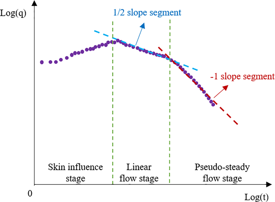
Figure 6: Schematic diagram of production-time double logarithmic curve
According to Bello’s theory [22] on the dual-porosity slab model in permeable fractures (Fig. 7), the model assumptions are as follows: ① Shale gas reservoirs are assumed to be closed rectangular gas reservoirs with multiple symmetrically distributed fractures. ② The length of the horizontal section of the gas well is considered to be the width of the gas reservoir. ③ The horizontal well is positioned at the center of the gas reservoir, and gas flows toward the center of the horizontal well. ④ The gas reservoir is modeled as a dual-porosity slab composed of fractures and matrix.
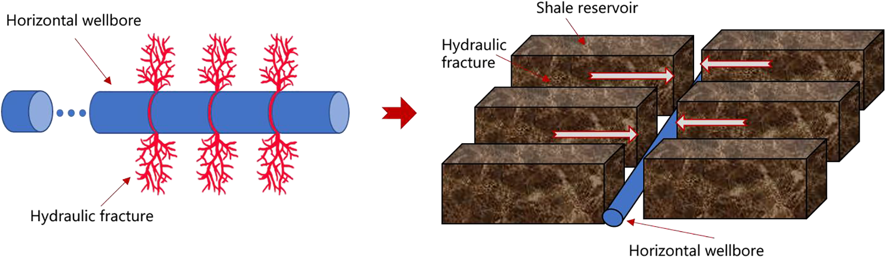
Figure 7: Schematic diagram of dual-porosity slab model
The gas well production solution of this model as follows:
Based on the bottom hole flow pressure data (
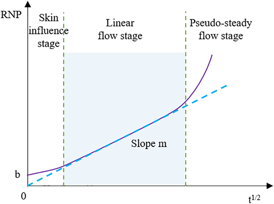
Figure 8: Schematic diagram of the relationship between rate normalized pressure and time
On the relationship curve between RNP and t1/2, an early linear segment can be observed. This linear segment represents the characteristic of the linear flow stage with a slope denoted as m. Therefore, a comprehensive parameter AcmKm1/2, reflecting the conductivity capability of shale gas wells during the flowback stage, can be obtained:
3.2 Processing and Analysis of Flowback Data
Due to the relatively long duration of simultaneous gas and water production during the flowback stage of shale gas wells and the significant pressure losses, for simplification in linear flow stage data analysis, the total equivalent surface flow rate of the well was obtained based on the instantaneous gas production rate qg and instantaneous water production rate qw recorded every hour during the flowback stage. This is achieved through the principles of equivalent surface flow [23], as detailed in the reference provided.
By substituting the total equivalent flow rate into Eqs. (3) and (4) in Section 3.1, and combining it with the choke size recorded every hour during the flowback stage, curve depicting the relationship between RNP and t1/2, as well as the relationship between choke size (CS) and t, were plotted (Fig. 9). These curves are used for qualitatively assessing the changes in shale gas well production capacity and whether the reservoir is effectively stimulated. The additional pressure losses caused by the early deviation from the linear segment in the curve results in an intercept value b on the curve with the vertical axis. As the choke is adjusted and production time increases, the intercept value b gradually decreases from slope ① to slope ④. This indicates an increase in the contact area between fractures and matrix, reflecting an improvement in reservoir cleanliness. During continuous production process, the gas well reaches the linear flow stage, showing a positively sloped line on the RNP and t1/2 curve. The slope m of this line provides the comprehensive parameter AcmKm1/2, reflecting the conductivity of the gas well during the flowback stage.
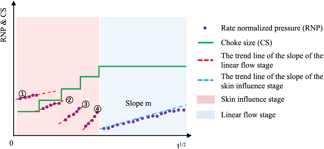
Figure 9: Schematic diagram of the relationship between rate normalized pressure and time, and the relationship between choke size and time (the red shaded parts ① to ④ in the figure represent the changes in different slope values; the blue shaded part represents the linear flow stage)
3.3 EUR Prediction Standard Chart for the Flowback Stage
The corresponding slope m for the linear flow stage was determined by analyzing the relationship curve between RNP and t1/2 for more than 120 deep shale gas wells in the Luzhou block. Using the formula for calculating AcmKm1/2, the AcmKm1/2 value of an actual gas well during the flowback process can be obtained, representing the comprehensive conductivity of the well during the flowback stage. By plotting a scatter plot of AcmKm1/2 against EUR for gas wells during the flowback stage, a good positive correlation was observed (Fig. 10). This indicates that the AcmKm1/2 value can be used to calculate the EUR of gas wells according to the relevant formula. The larger the AcmKm1/2 value during the flowback stage, the higher the EUR of the well. Therefore, it can be used to quantitatively assess the flowback effect of gas wells.
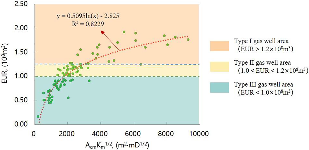
Figure 10: Relationship curve between AcmKm1/2 value and EUR during flowback stage of deep shale gas wells in the Luzhou block and the classification evaluation chart of gas wells
In order to realize rapid and accurate evaluation of the effect of deep shale gas well flowback stage in the Luzhou block, The EUR of gas wells was classified into Types I, II and III according to the interval classification, and the effect evaluation chart of shale gas well flowback stage in the Luzhou block was obtained (as shown in orange, yellow and green areas in Fig. 10). Among them, Type I gas wells represent good flowback effect with EUR greater than 1.2 × 10⁸ m3, Type II gas wells represent medium flowback effect with EUR between 1.0–1.2 × 10⁸ m3, and Type III gas wells represent poor flowback effect with EUR less than 1.0 × 10⁸ m3. By drawing the RNP vs. t1/2 curve of any shale gas well at the flowback stage in this block, the AcmKm1/2 value can be calculated, and the value can be compared with the Types I, II and III gas wells, enabling a rapid assessment of the flowback effect of the gas well.
This paper takes 84 shale gas wells in the Luzhou block with a long production history as statistical samples, and compares their actual EUR results in the production stage with the predicted EUR results in the flowback stage (Fig. 11). The results show that the deviation between the predicted EUR in the flowback stage and the actual EUR in the production stage is within ±2000 × 104 m3, and the average deviation is less than 1000 × 104 m3. The prediction error range of EUR is less than 20%, and the average error of EUR is 11%. The prediction of EUR in the flowback stage is reliable, and the error is within the acceptable range, which can support the effect evaluation of shale gas well in the Luzhou block. Simultaneously, it can provide reference for early investment estimation and reduce risks.
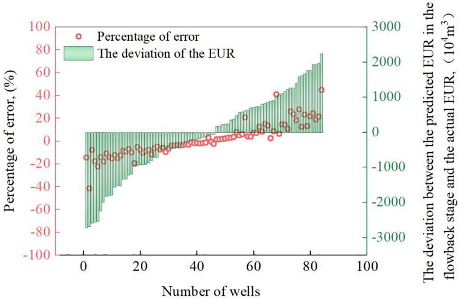
Figure 11: Comparison of the predicted EUR results in the flowback stage with the actual results
4 Analysis on Main Controlling Factors Influencing Gas Well EUR
By employing the evaluation method for the flowback stage of deep shale gas wells in the Luzhou block, rapid forecasting of EUR during the flowback stage of gas wells was achieved. In order to continuously track and evaluate the production effects of shale gas wells, understand the geological, engineering and production factors that affect the EUR of shale gas wells, and promptly support the adjustment of shale gas well production measures and the optimization of development technology strategies, it is urgent to analyze main controlling factors. The corresponding analysis process is shown in Fig. 12.
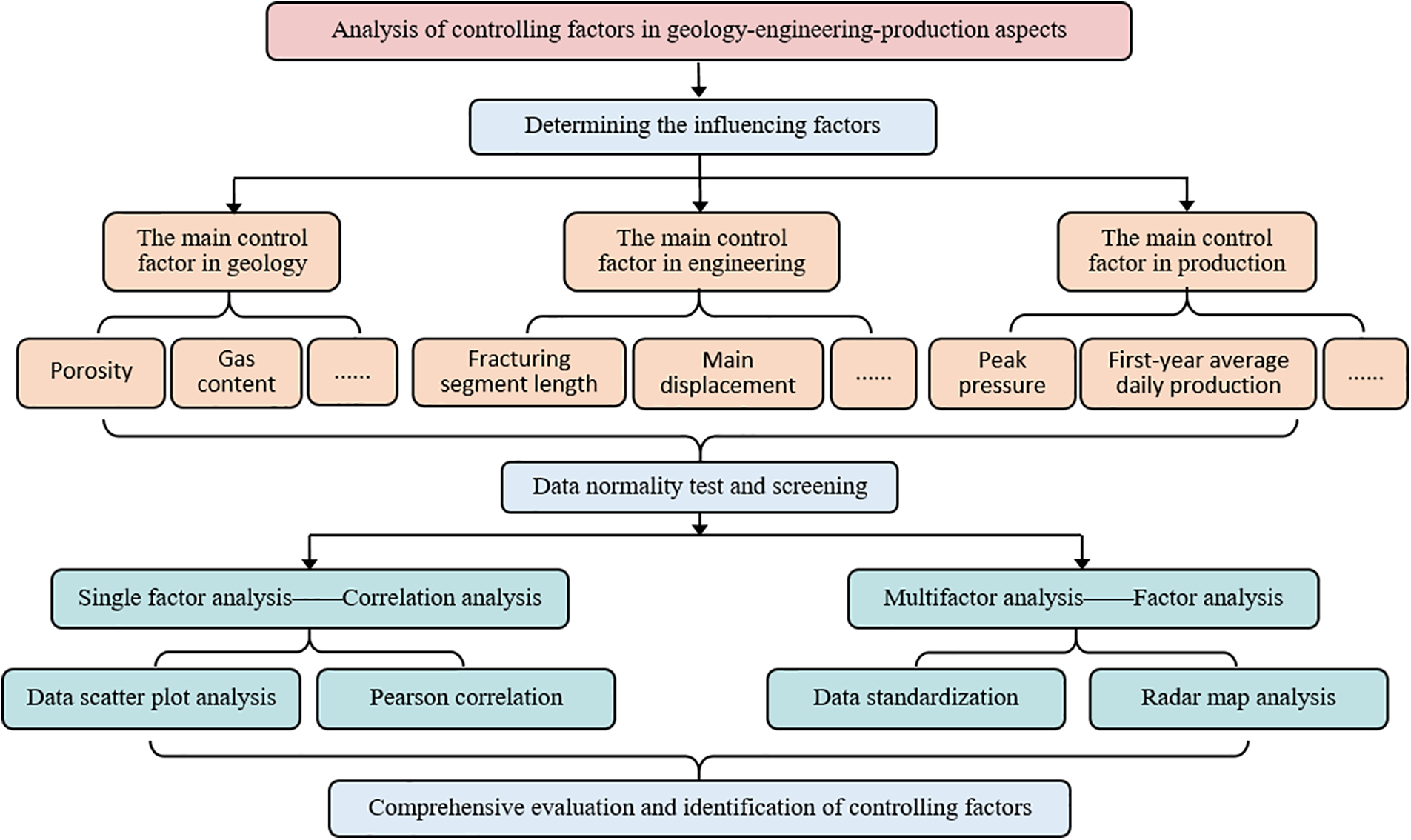
Figure 12: Analysis process of main control factors
4.1 Determining the Influencing Factors
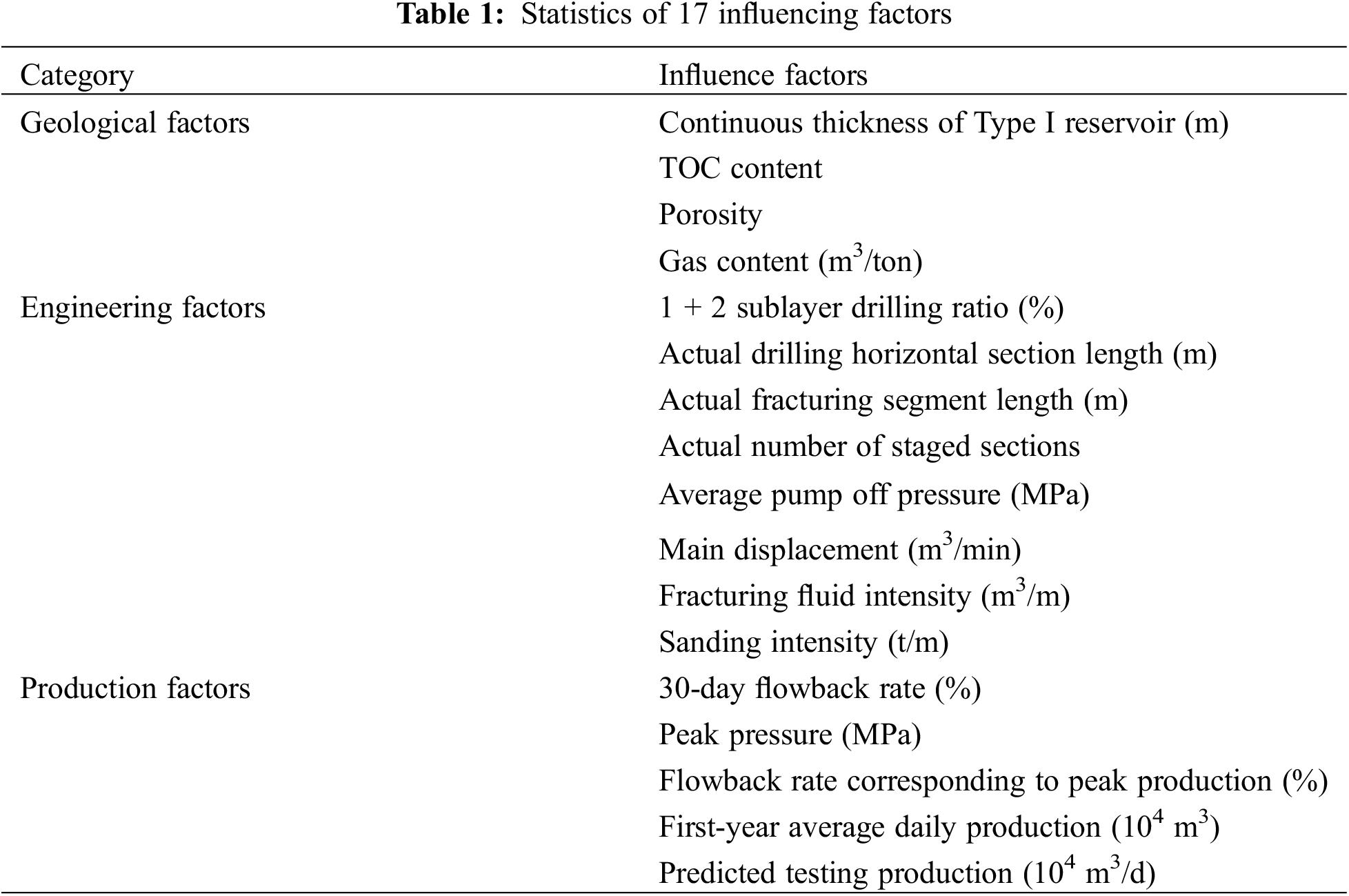
Based on the static and dynamic data of over 160 shale gas wells in the Luzhou block, 27 categories of geological, engineering, and production factors influencing shale gas well production were summarized. Utilizing big data analysis methods, the influencing degree of each factor on EUR was revealed. Geological factors include continuous thickness of Type I reservoir (Represents the continuous thickness of a high-quality reservoir), total organic carbon (TOC), brittle mineral content, porosity, gas saturation, and gas content. Engineering factors include drilling ratio, horizontal section length, fracturing segment length, cluster spacing, average pump pressure, main displacement, fracturing fluid intensity, and sanding intensity. Production factors include gas channeling time, peak pressure, first-year average daily production, and predicted testing production. Due to the multitude of influencing factors, it is crucial to effectively select statistically significant factors. Additionally, to eliminate dimensional differences between various factors, the data for analysis should be standardized.
Before analyzing the influencing factors and to ensure the reliability of the results, it is essential to filter out effective influencing factors. This is achieved by conducting a normal distribution test on the 27 categories of influencing factors through normal probability distribution plots (Figs. 13–15). From the figures, it is apparent that the data points of some categories do not align along a diagonal line, indicating a lack of conformity to normal distribution characteristics, and a relatively poor adaptability to further statistical analysis. Ultimately, 17 influencing factors that meet the analysis conditions were selected (Table 1).
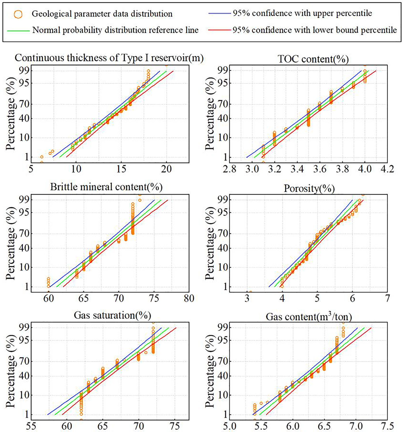
Figure 13: Normal probability distribution diagram of geological factors
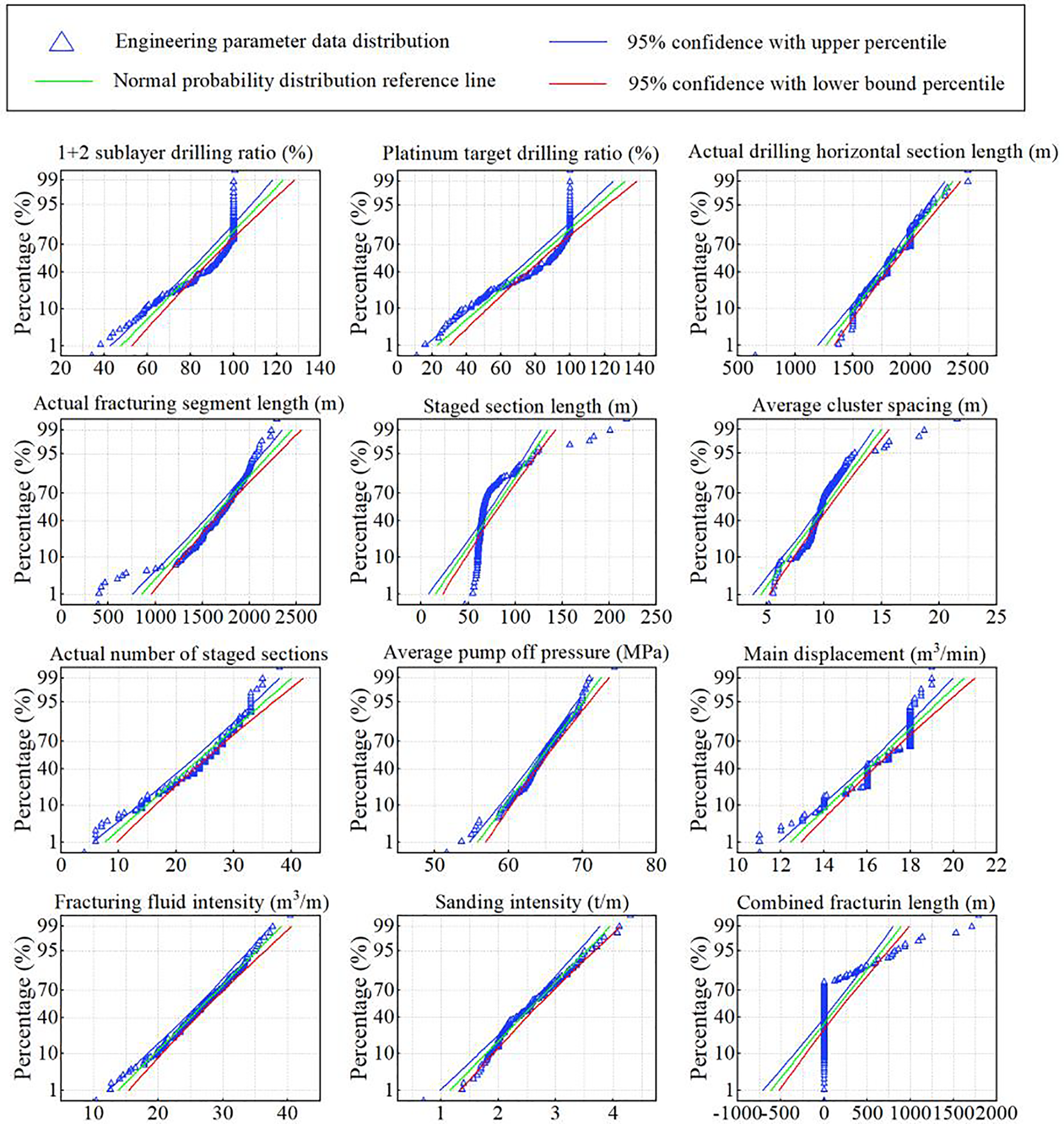
Figure 14: Normal probability distribution diagram of engineering factors
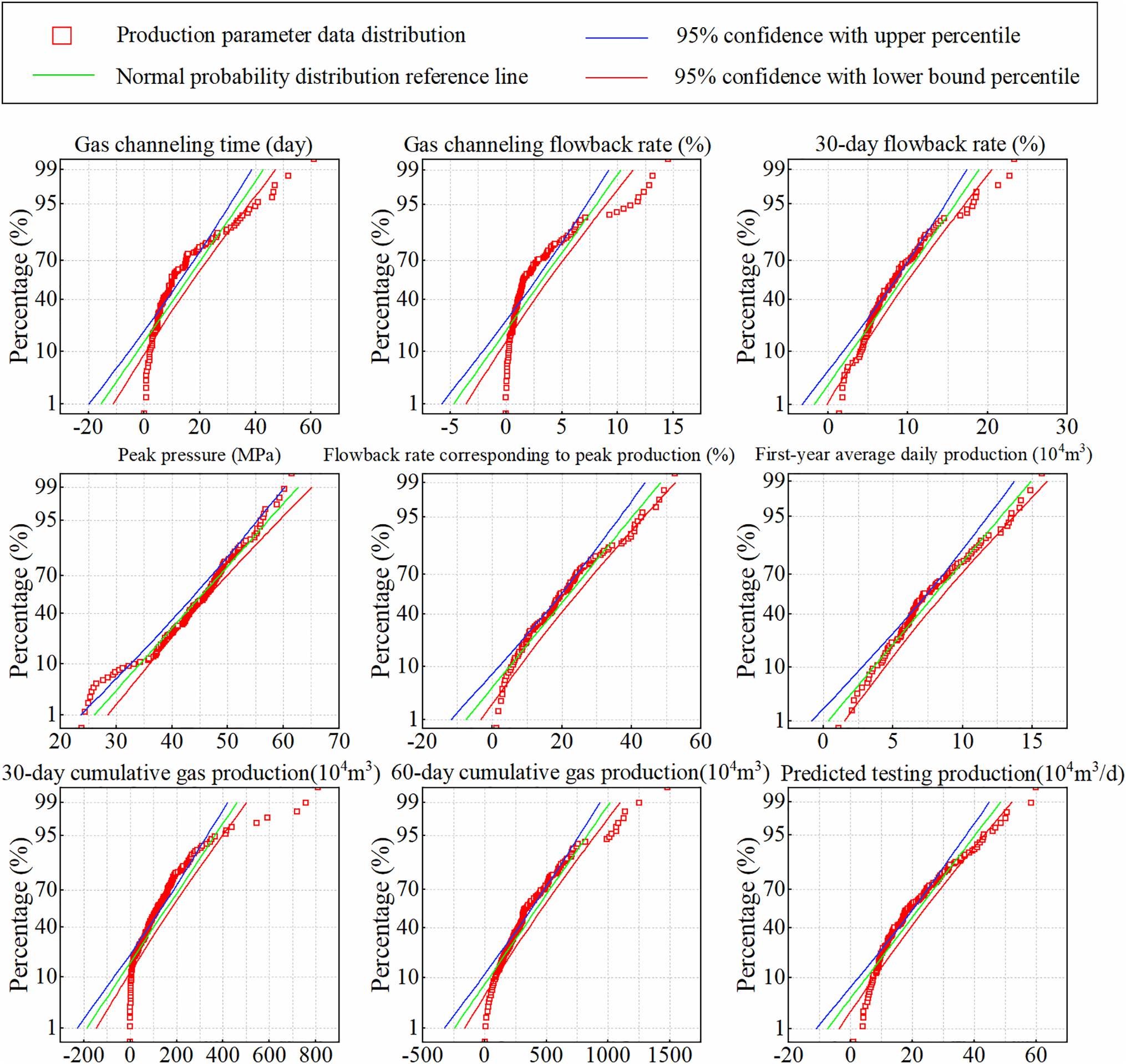
Figure 15: Normal probability distribution diagram of production factors
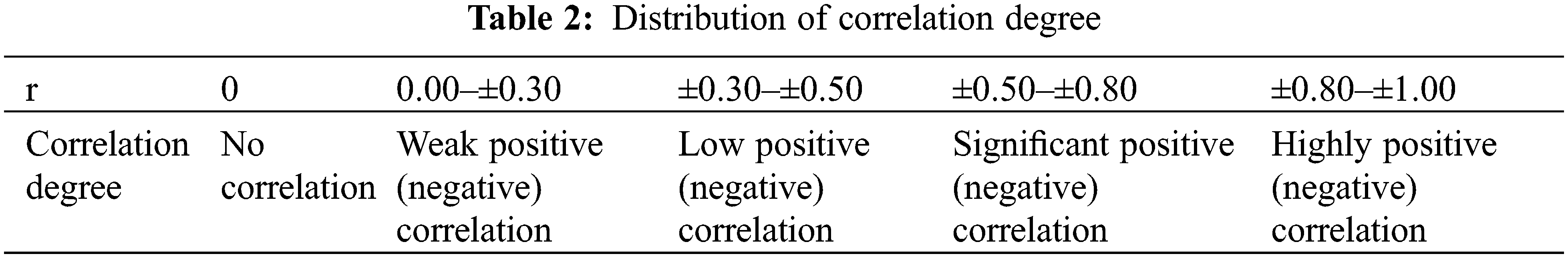
After conducting a normality test, 17 influencing factors were selected. The correlation coefficient, denoted as r, was introduced, which represents the linear correlation between two factors. The distribution values of the correlation coefficient are shown in Table 2, expressed as [24]
Through the correlation analysis on geological, engineering, and production factors of 160 shale gas wells in the Luzhou block, correlation distribution charts were obtained (Figs. 16–18). The correlation degree is illustrated in Fig. 19. It can be observed from the figures that the correlation between individual factors and gas well EUR is relatively low, indicating that a single factor alone cannot fully characterize the influence on gas well EUR.
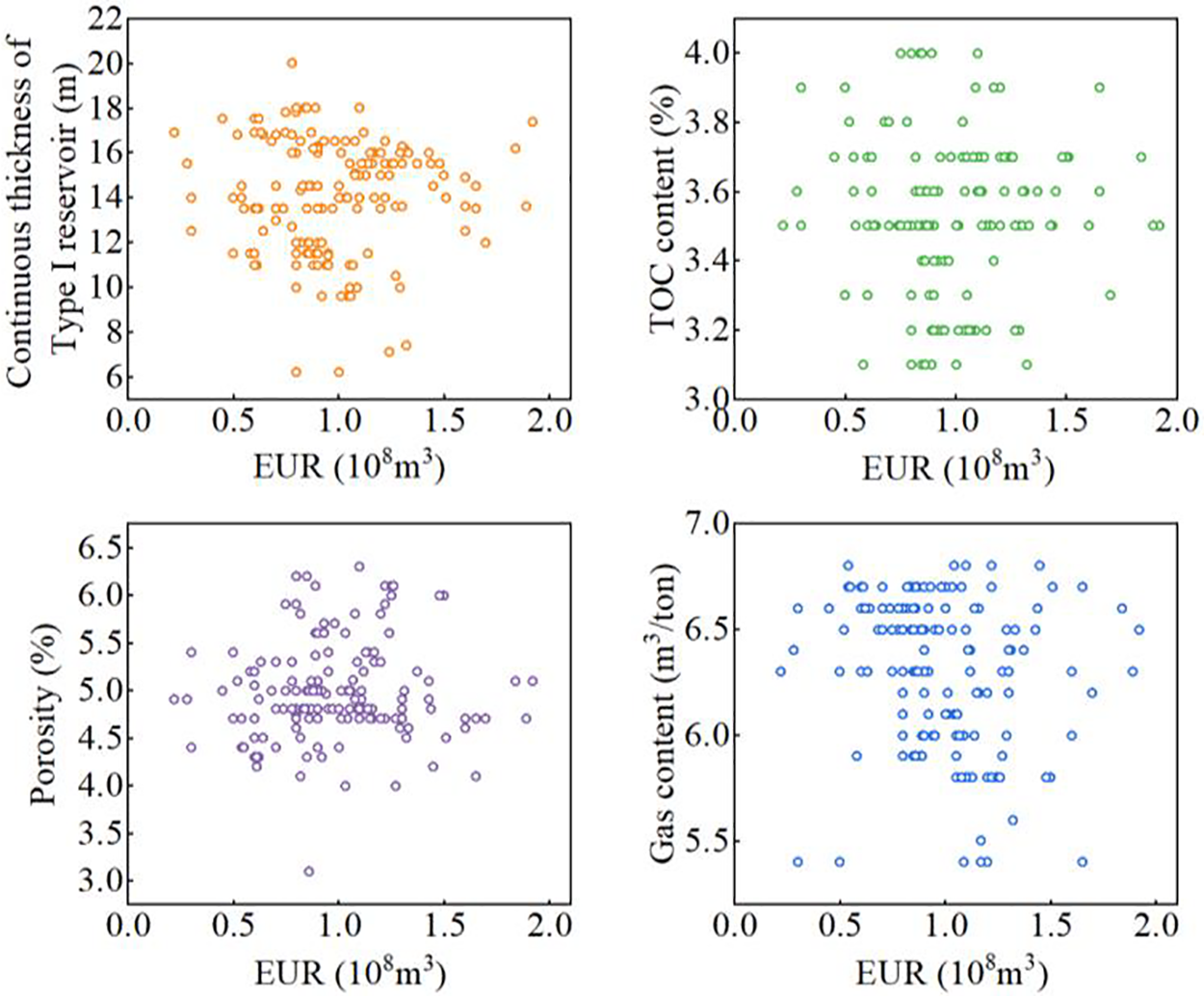
Figure 16: Distribution diagram of correlation between geological factors and EUR
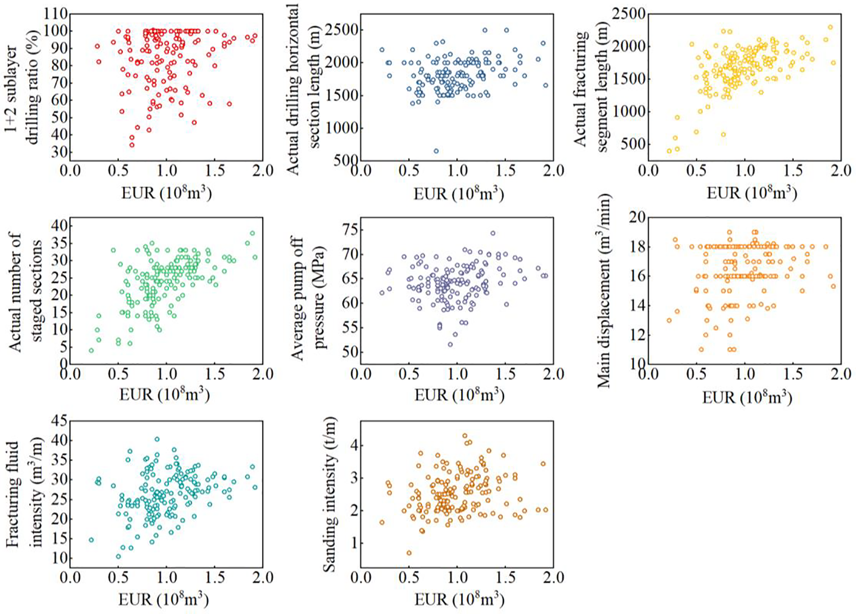
Figure 17: Distribution diagram of correlation between engineering factors and EUR
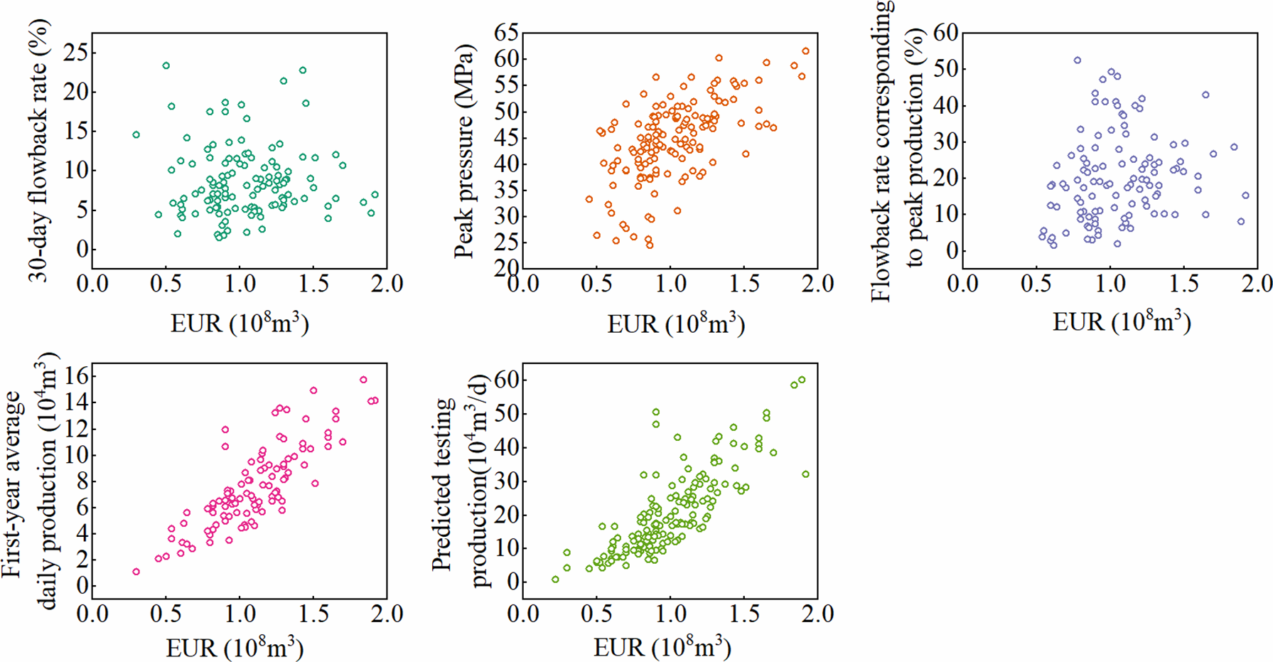
Figure 18: Distribution diagram of correlation between production factors and EUR
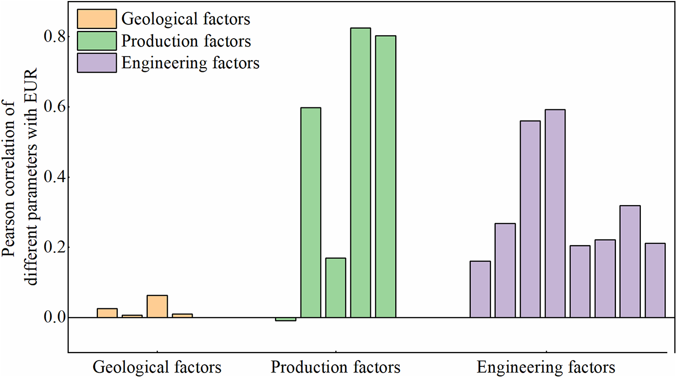
Figure 19: Distribution diagram of the correlation between different parameters and EUR
There are numerous types of influencing factors, which introduces uncertainty to the analysis of main controlling factors and increases the complexity of problem-solving. Therefore, in this study, a “dimensionality reduction” approach was employed using the factor analysis method [25]. This method extracts common factors to enhance analysis efficiency and uncover the main controlling factors influencing gas well EUR.
According to the factor extraction conditions, a scree plot was generated through principal component analysis, and the number of the factors with eigenvalues greater than 1 was considered as the extracted number of factors (Fig. 20). Five factors were extracted, which can effectively represent the influence of the original 17 categories of factors. An analysis of the rotated loadings for the 5 factors is presented in Table 3. To differentiate the primary influencing factors reflected by each factor, radar charts (spider charts) were created for each factor with the 17 categories of influencing factors (Fig. 21). A visual observation of the series of influencing factors reflected by each factor was facilitated. Factor 1 mainly reflects the influence of first-year average daily production, peak pressure, and predicted testing production, representing the factor influencing the initial production capacity of gas wells. Factor 2 mainly reflects the influence of horizontal section length and fracturing segment length, representing the factor influencing the well control range of gas wells. Factor 3 mainly reflects the influence of Type I reservoir thickness and TOC content, representing the factor influencing the reservoir quality. Factor 4 mainly reflects the influence of sanding intensity and fracturing fluid intensity, representing the factor influencing the fracturing scale of gas wells. Factor 5 mainly reflects the influence of porosity and gas content, representing the factor influencing the gas-bearing capacity of gas wells.
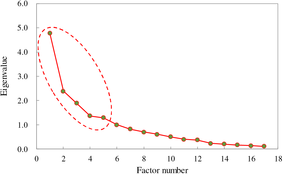
Figure 20: Scree plot of extracted principal component factor
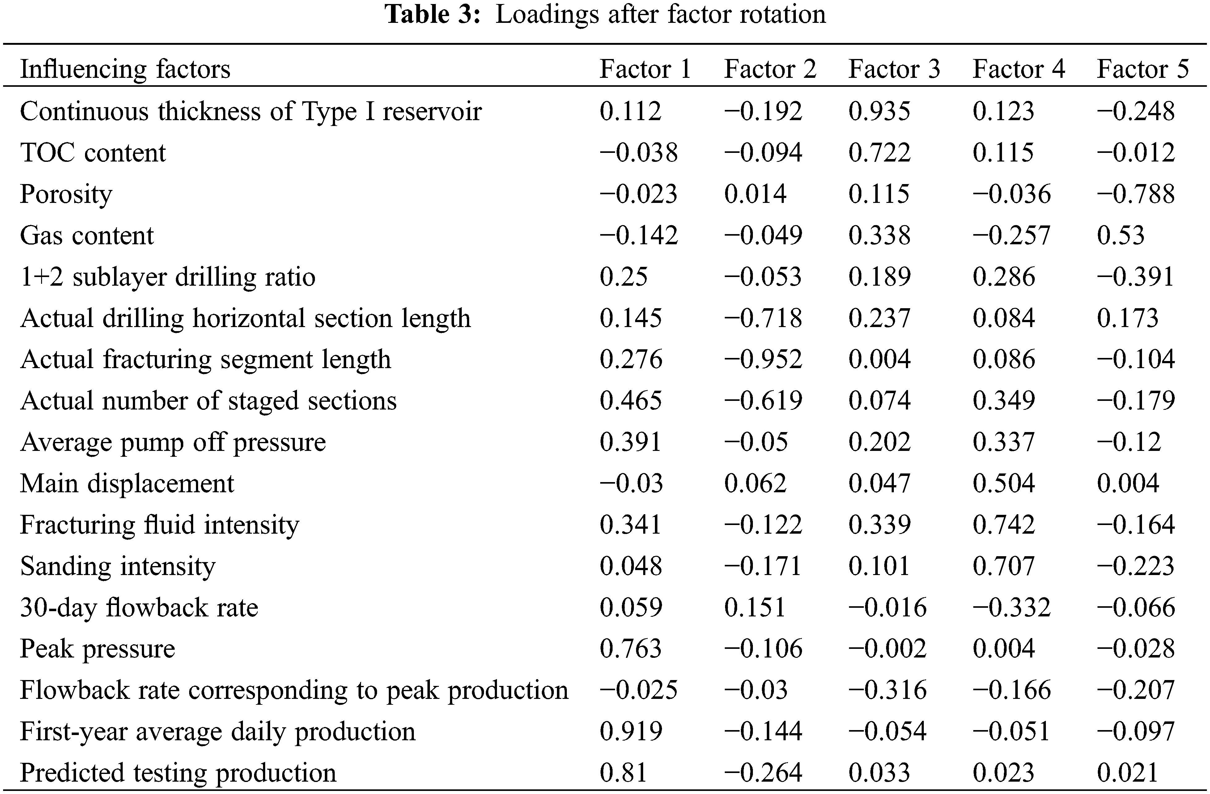
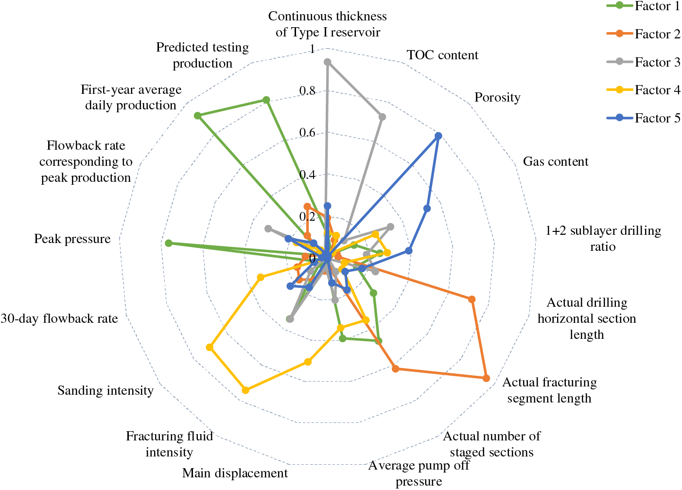
Figure 21: Radar chart from factor analysis
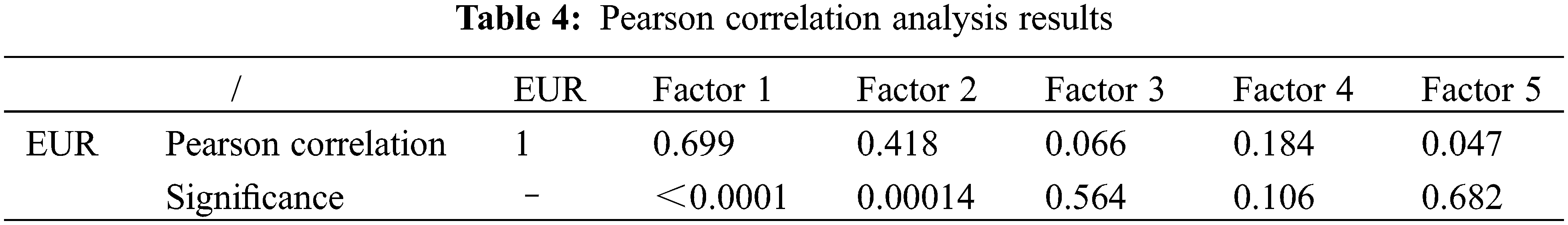
To analyze the correlation between the 5 factors and EUR, Pearson correlation analysis was conducted (Table 4). The results indicate that Factor 1 and Factor 2 have a significant correlation with EUR. This suggests that the performance of shale gas wells in this deep block is significantly influenced by well control range and initial production capacity. Therefore, to enhance gas well production and EUR, it is advisable to further explore reasonable well spacing in the development well pattern and optimize initial drainage and production techniques.
The shale gas well H1 in the Luzhou block has horizontal section length of 2000 m, initial reservoir pressure
Based on the instantaneous gas production rate
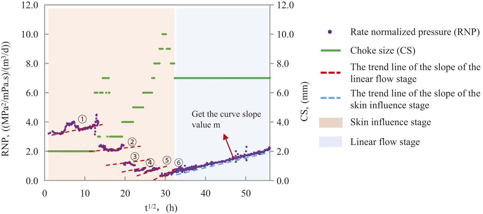
Figure 22: The relationship curves between rate normalized pressure and time, choke size and time for well H1 (the red shaded parts ① to ⑥ in the figure represent the changes in different slope values; the blue shaded part represents the linear flow stage)
As the choke size of the well gradually increases, the corresponding RNP values decrease, indicating an enhancement in the production capacity of gas wells. Simultaneously, the slope of the curve decreases gradually from ① to ⑥, becoming flatter, and the intercept value b decreases, indicating an increase in the contact area between fractures and matrix, which means the reservoir is stimulated effectively. By calculating the slope m of the upper linear flow stage as 181.314 MPa²/((mPa·s)·m³/h·h1/2), the AcmKm1/2 value for this well during the flowback process was determined to be 1488 m²·mD1/2. Based on the relationship chart between AcmKm1/2 and EUR calculated during the flowback stage for this block (Fig. 10), the EUR value of this well was estimated to be 0.9 × 10⁸ m3, so the well is classified as a Type III gas well.
(1) The typical flowback curve for deep shale gas wells is primarily divided into three stages: before gas channeling, before reaching peak pressure, and after reaching peak pressure. In comparison with early flowback indicators for mid-deep wells, it generally exhibits the characteristics of later gas channeling, higher gas flowback rate after gas channeling, lower 30-day flowback rate, and higher flowback rate corresponding to peak production.
(2) After analyzing the linear flow model for shale gas wells, combined with the equivalent flow processing during the flowback stage, the comprehensive parameter AcmKm1/2 for more than 120 deep shale gas wells in the flowback stage were tracked, analyzed, and calculated. A relationship chart between AcmKm1/2 and gas well EUR was established, and gas well types were classified, enabling rapid prediction of gas well EUR during the flowback stage.
(3) By using big data statistical analysis methods, combined with dynamic and static data from over 160 deep gas wells on site, through cleaning and dimensionality reduction of the data, influencing factors was analyzed. It indicates that the performance of gas wells is greatly affected by the well control range and initial production capacity, and further exploring reasonable well pattern and well spacing and further optimizing initial drainage and production strategies are crucial for enhancing individual well performance and achieving large-scale benefit development of deep shale gas wells.
Acknowledgement: All authors are grateful for the hard work of the journal editorial office and the dedication of the unconventional oil and gas exploration and development personnel.
Funding Statement: This research did not receive any specific grant from funding agencies in the public, commercial, or not-for-profit sectors.
Author Contributions: The authors confirm contribution to the paper as follows: Data curation, Formal analysis, Writing–original draft: Sha Liu. Conceptualization, Project administration, Writing–review & editing: Jianfa Wu and Xuefeng Yang. Data curation: Cheng Chang. Modify details, Method validation: Weiyang Xie. All authors reviewed the results and approved the final version of the manuscript.
Availability of Data and Materials: The data that support the findings of this study are available from the Shale Gas Research Institute of PetroChina Southwest Oil and Gas Field Company. Restrictions apply to the availability of these data, which were used under license for this study. Data are available from the authors with the permission of the Shale Gas Research Institute of PetroChina Southwest Oil and Gas Field Company.
Conflicts of Interest: The authors declare that they have no conflicts of interest to report regarding the present study.
References
1. Zhao J, Ren L, Jiang T, Hu D, Wu L, Wu J, et al. Ten years of gas shale fracturing in China: review and prospect. Nat Gas Ind. 2021;41(8):121–42 (In Chinese). doi:10.3787/j.issn.1000-0976.2021.08.012. [Google Scholar] [CrossRef]
2. Xu F, Wang F, Zhang J, Fu B, Zhang Y, Yang P, et al. Strategies for scale benefit development of deep shale gas in China. Nat Gas Ind. 2021;41(1):205 (In Chinese). doi:10.3787/j.issn.1000-0976.2021.01.019. [Google Scholar] [CrossRef]
3. Ma Z, Xiao H. Study on the development strategy of shale gas industry in China from the perspective of energy revolution. Energy China. 2017;39(11):5 (In Chinese). [Google Scholar]
4. Williams-Kovacs JD, Clarkson CR. A modified approach for modeling two-phase flowback from multi-fractured horizontal shale gas wells. J Nat Gas Sci Eng. 2016;30:127–47. doi:10.1016/j.jngse.2016.02.003. [Google Scholar] [CrossRef]
5. Xue X, Liu S, Leiker C. Early EUR indicator for permian basin unconventional resources based on hourly flowback data. In: SPE/AAPG/SEG Unconventional Resources Technology Conference; 2023 Jun; Denver, Colorado, USA. doi:10.15530/urtec-2023-3854193. [Google Scholar] [CrossRef]
6. Aldana IC, Akkutlu IY, Lee WJ. Bilinear flow analysis of shale gas wells with dynamic hydraulic fracture conductivity. In: SPE/AAPG/SEG Unconventional Resources Technology Conference; 2023 Jun; Denver, Colorado, USA. doi:10.15530/urtec-2023-3862595. [Google Scholar] [CrossRef]
7. De Oliveira Werneck R, Prates R, Moura R, Gonçalves M, Castro M, Soriano-Vargas A, et al. Data-driven deep-learning forecasting for oil production and pressure. J Pet Sci Eng. 2022;210:109937. doi:10.1016/j.petrol.2021.109937. [Google Scholar] [CrossRef]
8. Liu J, He X, Huang H, Yang J, Dai J, Shi X, et al. Predicting gas flow rate in fractured shale reservoirs using discrete fracture model and GA-BP neural network method. Eng Anal Bound Elem. 2024;159:315–30. doi:10.1016/j.enganabound.2023.12.011. [Google Scholar] [CrossRef]
9. Chen X, Ou Y, Qu Z, Tang X, Luo X, He J. A new method for productivity prediction at the initial stage of production of shale gas wells. Drill Prod Technol. 2023;46(4):77–81 (In Chinese). doi:10.3969/J.ISSN.1006-768X.2023.04.13. [Google Scholar] [CrossRef]
10. Altwaijri M, Xia Z, Yu W, Qu L, Xu Y, Xu Y, et al. Numerical study of complex fracture geometry effect on two-phase performance of shale-gas wells using the fast EDFM method. J Pet Sci Eng. 2018;164:603–22. doi:10.1016/j.petrol.2017.12.086. [Google Scholar] [CrossRef]
11. Liu J, Qiu X, Yang J, Liang C, Dai J, Bian Y. Failure transition of shear-to-dilation band of rock salt under triaxial stresses. J Rock Mech Geotech Eng. 2024;16(1):56–64. doi:10.1016/j.jrmge.2023.03.015. [Google Scholar] [CrossRef]
12. Yang J, Liu J, Li W, Dai J, Xue F, Zhuang X. A multiscale poroelastic damage model for fracturing in permeable rocks. Int J Rock Mech Min Sci. 2024;175:105676. doi:10.1016/j.ijrmms.2024.105676. [Google Scholar] [CrossRef]
13. Makhanov K, Habibi A, Dehghanpour H, Kuru E. Liquid uptake of gas shales: a workflow to estimate water loss during shut-in periods after fracturing operations. J Unconv Oil Gas Resour. 2014;7:22–32. doi:10.1016/j.juogr.2014.04.001. [Google Scholar] [CrossRef]
14. Benson ALL, Clarkson CR. Flowback rate-transient analysis with spontaneous imbibition effects. J Nat Gas Sci Eng. 2022;108:104830. doi:10.1016/J.JNGSE.2022.104830. [Google Scholar] [CrossRef]
15. He X, Chen G, Wu J, Liu Y, Wu S, Zhang J, et al. Deep shale gas exploration and development in the southern Sichuan Basin: new progress and challenges. Nat Gas Ind B. 2023;10(1):32–43. doi:10.1016/J.NGIB.2023.01.007. [Google Scholar] [CrossRef]
16. Long S, Lu T, Li Q, Yang G, Li D. Discussion on China’s shale gas development ideas and goals during the 14 five-year plan. Nat Gas Ind. 2021;41(10):1–10 (In Chinese). doi:10.3787/j.issn.1000-0976.2021.10.001. [Google Scholar] [CrossRef]
17. He X, Li W, Dang R, Huang S, Wang X, Zhang C, et al. Key technological challenges and research directions of deep shale gas development. Nat Gas Ind. 2021;41(1):118–24 (In Chinese). doi:10.3787/j.issn.1000-0976.2021.01.010. [Google Scholar] [CrossRef]
18. Tan B. Key technologies and prospects of deep shale gas engineering in the southern Sichuan Basin. Nat Gas Ind. 2022;42(8):212–9 (In Chinese). doi:10.3787/j.issn.1000-0976.2022.08.017. [Google Scholar] [CrossRef]
19. Yu G, Liu H, Li H, Fang Y, Luo L. Prediction on peak production of shale gas, Southern Sichuan Basin. Nat Gas Explor Dev. 2023;46(1):97–104 (In Chinese). doi:10.12055/gaskk.issn.1673-3177.2023.01.012. [Google Scholar] [CrossRef]
20. Anderson DM, Nobakht M, Moghadam S, Mattar L. Analysis of production data from fractured shale gas wells. In: SPE Unconventional Gas Conference; 2010 Feb; Pittsburgh, PA, USA. doi:10.2523/131787-MS. [Google Scholar] [CrossRef]
21. Wattenbarger RA, El-Banbi AH, Villegas ME, Maggard JB. Production analysis of linear flow into fractured tight gas wells. In: SPE Rocky Mountain Regional/Low-Permeability Reservoirs Symposium; 1998 Apr; Denver, CA, USA. doi:10.2118/39931-MS. [Google Scholar] [CrossRef]
22. Bello RO, Wattenbarger RA. Multi-stage hydraulically fractured horizontal shale gas well rate transient analysis. In: SPE North Africa Technical Conference and Exhibition; 2010 Feb 14–17; Cairo, Egypt. doi:10.2118/126754-MS. [Google Scholar] [CrossRef]
23. Perrine RL. Analysis of pressure buildup curves. Drill Prod Pract. 1956:482–509. [Google Scholar]
24. Adler J, Parmryd I. Quantifying colocalization by correlation: the Pearson correlation coefficient is superior to the Mander’s overlap coefficient. Cytom Part A. 2010;77(8):733–42. doi:10.1002/cyto.a.20896. [Google Scholar] [PubMed] [CrossRef]
25. Wang W, Chen X. Comparison of principal component analysis with factor analysis in comprehensive multi-indicators scoring. Stat Inform Forum. 2006;21(5):19–22 (In Chinese). doi:10.3969/j.issn.1007-3116.2006.05.004. [Google Scholar] [CrossRef]
Cite This Article
 Copyright © 2024 The Author(s). Published by Tech Science Press.
This work is licensed under a Creative Commons Attribution 4.0 International License , which permits unrestricted use, distribution, and reproduction in any medium, provided the original work is properly cited.
 Downloads
 Citation Tools