
 Submit a Paper
 Propose a Special lssue
 Open Access
ARTICLE

Simulation of the Production Performances of Horizontal Wells with a Fractured Shale Gas Reservoir
1 Sichuan Changning Natural Gas Development Co., Ltd., Chengdu, 610041, China
2 State Key Laboratory of Oil & Gas Reservoir Geology and Exploitation, Southwest Petroleum University, Chengdu, 610500, China
3 Chengdu North Petroleum Exploration and Development Technology Company Limited, Chengdu, 610051, China
* Corresponding Authors: Ruihan Zhang. Email: ; Xin Huang. Email:
Fluid Dynamics & Materials Processing 2023, 19(7), 1803-1815. https://doi.org/10.32604/fdmp.2023.026143
Received 18 August 2022; Accepted 08 November 2022; Issue published 08 March 2023
 View Full Text
 Download PDF
Abstract
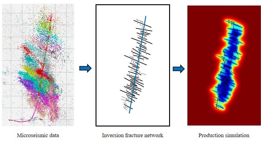
The production performances of a well with a shale gas reservoir displaying a complex fracture network are simulated. In particular, a micro-seismic cloud diagram is used to describe the fracture network, and accordingly, a production model is introduced based on a multi-scale flow mechanism. A finite volume method is then exploited for the integration of the model equations. The effects of apparent permeability, conductivity, Langmuir volume, and bottom hole pressure on gas well production are studied accordingly. The simulation results show that ignoring the micro-scale flow mechanism of the shale gas leads to underestimating the well gas production. It is shown that after ten years of production, the cumulative gas production difference between the two scenarios with and without considering the micro-scale flow mechanisms is 19.5%. The greater the fracture conductivity, the higher the initial gas production of the gas well and the cumulative gas production. The larger the Langmuir volume, the higher the gas production rate and the cumulative gas production. With the reduction of the bottom hole pressure, the cumulative gas production increases, but the growth rate gradually decreases.Graphic Abstract
Keywords
Shale gas reservoirs with rich reserves, as an important supplement to the energy supply, have become a focus of global development in recent years [1]. Compared with conventional gas reservoirs, shale gas reservoirs are extremely tight and require the use of long horizontal wells and hydraulic fracturing to obtain industrial production. This leads to the fluids flowing through the nano/micro-pores, and the small- and large-scale fractures having multi-scale flow characteristics [2–5].
Fractures in shale have various types and scales, including micro-scale natural fractures and large-scale hydraulic fractures. Fractures can serve as both storage space and transport channels for free gas in shale, and they provide effective flow channels, increasing the effective porosity and permeability of the reservoir. Therefore, reservoir characterization and geological modeling of shale gas reservoirs require the fine portrayal and modeling of fractures. When predicting the production performance of fractured horizontal wells in shale gas reservoirs, the characterization of the complex fracture network is the key to obtaining the most accurate results [6–10]. Currently, in most studies, the hydraulic fractures were set as simple straight and flat fractures, and the characterization of the fractures was relatively simple, which can easily lead to deviation of the results from the actual situation. On-site microseismic monitoring data provide a more accurate representation of the underground fracturing situation. The fractures interpreted using microseismic data can more accurately represent the shape of the fractures formed via hydraulic fracturing.
In recent years, researchers have studied the production performance of post-fracturing horizontal wells from three aspects, i.e., analytical models [11–13], semi-analytical models [14–16], and numerical models, and have provided suggestions for optimization of the production system. Both analytical and semi-analytical models are too simplified, resulting in a large deviation from the actual reservoir situation. Due to the complexity of the fracture distribution, a fracture model that uses an equivalent continuous model is a highly simplified version of the real formation, and this simplification inevitably leads to loss of the actual subsurface fracture details. Due to the strong heterogeneity of fractured reservoirs and multi-scale fractures, the assumptions of the equivalent continuous model are not acceptable in many cases. Moreover, an equivalent continuous model cannot well characterize the anisotropic features in reservoirs.
To overcome these problems, a series of numerical models have been developed by researchers. Composite reservoir models based on continuum media have been proposed to numerically predict the flow mechanisms in shale gas reservoirs, but they are only appropriate for reservoirs with small-scale fractures [17]. Thus, considering the limitation in describing the multi-scale fractures in shale, the discrete-fracture model (DFM), the coupled continuum media model, and the discrete-fracture model were successively established to achieve flexibility in simulating complex fracture geometries [18,19]. However, the simulation results of these methods are obtained using unstructured grids, and the establishment of unstructured grids is more complex than the establishment of traditional orthogonal grids.
In addition, in the above numerical models, the fracture network is characterized by random simulation, which makes it difficult to guarantee the correctness of the predicted production of the gas wells. When using numerical simulation or commercial software to deal with the fracture system, the grid around the fracture needs to be refined, which increases the number of calculations in the numerical simulation and increases the calculation time. The embedded discrete fracture model embeds the fracture attributes into the matrix grid, divides the calculation area using a structural grid, reduces the number of grids, and does not need to refine the fractures [20]. It has good adaptability to fractured horizontal wells with complex fracture shapes and better calculation efficiency. Microseismic data can directly display the fracture morphology in fractured horizontal wells, and inversion of the fracture geometry using microseismic data has good accuracy [21].
In summary, in this study, a micro-seismic cloud map was used to characterize the actual shapes of hydraulic fractures. By considering the comprehensive flow mechanisms of shale gas, including the flow through micro-scale pores, isothermal adsorption, and desorption characteristic, as well as the stress sensitivity of the fractures, a mathematical model of gas reservoir seepage was established based on the embedded discrete fracture model. A numerical solution model was established using a structured grid and the finite volume method. Using on-site data, the production performance of horizontal wells after fracturing was simulated and predicted, and the factors affecting the gas well production and stimulation effect were analyzed.
After fracturing, shale reservoirs form complex fracture network zones, including fracture systems with multi-scale characteristics [22]. An accurate description of the fracture system is the most crucial key to improving production performance of fractured horizontal wells in shale gas reservoirs.
Through on-site microseismic monitoring, it was found that there are dense signal response points around a fractured horizontal well. Through interpretation and processing of the fracturing monitoring data, an embedded discrete fracture model based on microseismic data for multi-stage fractured horizontal wells in shale reservoirs was constructed.
The main steps for constructing a discrete fracture model based on microseismic monitoring data are as follows:
Step 1: Interpret and process the microseismic data collected during the fracturing process, and record the important parameters, including the number of fracturing segments, fracturing construction time, spatial location, and signal amplitude.
Step 2: Combine the geological and geophysical data, pre-process the relevant parameters, and eliminate unreasonable microseismic points generated during monitoring of surface or shallow wells.
Step 3: Combine the borehole trajectory and shot hole data and reconstruct the fracture network system using an iterative algorithm for each level of the fractured section.
Step 4: Superimpose the fracture networks of the fractured sections at each level in turn to form the overall fracture network of the fractured horizontal wells and establish a discrete fracture network model.
Step 5: Match the historical production data to the numerical simulation prediction results obtained using the discrete fracture network model to modify the fracture property parameters and fracture distribution.
The following assumptions were made in the physical model (Fig. 1). (1) The reservoir flow process is gas-phase isothermal flow. (2) The vertical heterogeneity of the reservoir is ignored and structured grids are used to describe the planar features. (3) The gas flows through the reservoir matrix into the fractures and then flows into the wellbore.
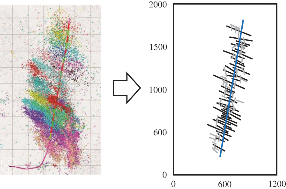
Figure 1: Model of a fractured horizontal well with a complex fracture network in a shale gas reservoir based on the micro-seismic cloud map [23] and the discrete fracture model. The blue, black, and grey lines denote the wellbore, hydraulic fractures, and secondary fractures, respectively. The simulation area is divided into 120 × 200 square grids
3 Mathematical and Numerical Models
3.1 Micro-Scale Flow Model for a Shale Gas Reservoir
Shale reservoirs have a complex pore structure, and the gas seepage in shale reservoirs has multiple flow mechanisms such as Knudsen diffusion, surface adsorption diffusion, slip flow, and viscous flow (Fig. 2) [24–26].
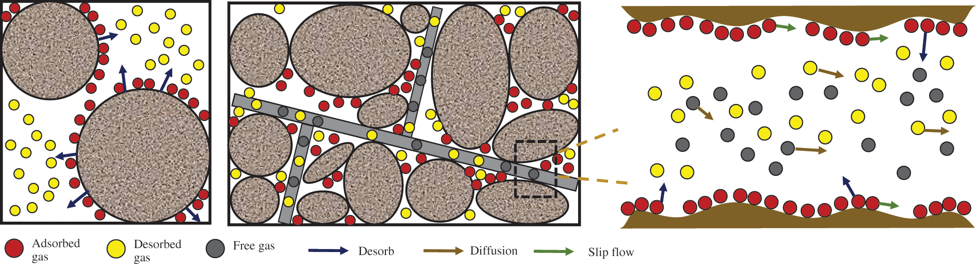
Figure 2: Migration mechanisms of shale gas in micro- and nano-scale pores
The molar mass flux of Knudsen diffusion is as follows:
where r is the pore radius in the shale reservoir (m); Mg is the molar mass of the gas (kg/mol); R is the gas constant (8.314 J/(mol•K)); T is the temperature of the shale reservoir (K); and p is the gas pressure in the pores (MPa).
The molar mass flux of surface adsorption diffusion is as follows:
where Ds is the surface diffusion coefficient (m2/s); Φ is the porosity; and Cu is the concentration of the adsorbed gas (mol/m3).
The molar mass flux of viscous flow is as follows:
where μ is the viscosity of the gas (mPa•s); and Z is the gas compression factor.
The molar mass flux of slip flow is as follows:
where Kn is the Knudsen diffusion constant; α is the rarefaction coefficient; and β is the slip factor.
For Knudsen diffusion and slip flow, a weighting factor is introduced to characterize their contributions to the total gas flow [27]. The total molar mass flux of the gas in a single capillary of a shale nanopore can be calculated as follows:
where εH is the weighting factor of the slip flow; εK is the weighting factor of the Knudsen diffusion; Vstd is the volume of gas in the standard state (m3/mol); and VL is the Langmuir volume (m3/kg).
Based on the expression of the molar mass flux of Darcy seepage, the apparent permeability of the gas shale, considering the microscopic seepage mechanism, can be obtained from Eq. (5) as follows:
Taking into account the reduction of the nanopore size due to the gas adsorption effect, the effective pore size is as follows:
where dc is the molecular diameter of the gas (m); and pL is the Langmuir pressure (MPa).
The apparent permeability of the shale considering the pore tortuosity can be obtained by combining Eqs. (6) and (7):
3.2 Embedded Discrete Fracture Model
The continuity equation for the gas flow in the reservoir is
where Φ is the porosity; and ρg is the density of the gas (kg/m3).
The equations of motion for gas are
where ρgsc is the density of the gas under standard conditions (kg/m3).
By combining Eqs. (9) and (12), the material balance equation can be obtained as follows:
The form of Eq. (13) for a matrix system is as follows:
The form of Eq. (13) for a fracture system is as follows:
where Ψ is the conductivity between the different systems.
The conductivity between the fracture and matrix is
For both the matrix and fracture systems, the conductivity satisfies the following relationship:
where CI is the connection pair between the different systems.
The connection pair between the matrix and fracture is as follows:
where kij,k is the harmonic average of the permeability of matrix grid ij and fracture segment k; and Aij,k is the contact area between matrix grid ij and fracture segment k. dij,k is the average distance from a point within matrix grid ij to fracture segment k, and it can be calculated as follows:
The conductivity between two fractures is
The connection pair between the two fractures is as follows:
where kfi is the fracture permeability; wfi is the fracture aperture; dfi is the distance from the center of the fracture segment to the fracture intersection line; and Lint is the length of the intersection line.
According to Gauss’s theorem and the finite volume method, Eq. (14) can be discretized as follows:
where ΔAx and ΔAy are the surface areas of the structured grid in the x and y directions, respectively.
Similarly, according to Gauss’s theorem and the finite volume method, Eq. (15) can be discretized as follows:
where Δxf is the discrete length of the fracture segment; and ΔAf is the fracture aperture.
Eqs. (23) and (24) can be written in matrix form as follows:
The outer boundary of the shale reservoir is closed, and the inner boundary is set for constant bottom-hole pressure production. The Gauss-Seidel iteration method is used to solve Eq. (25).
4 Simulation Results and Sensitivity Analysis
Jiang et al. [28] simulation results for a scenario with a complex fracture network were selected to validate our model. The size of the reservoir was set as 400 m × 300 m × 20 m, the initial reservoir pressure was 14 MPa, the bottom hole pressure was 4 MPa, and the matrix permeability was 2 × 10⁻⁵ mD. The hydraulic fracture permeability was 500 mD, and the fracture width was 0.003 m. The complex fracture model of the horizontal well is shown in Fig. 3a.
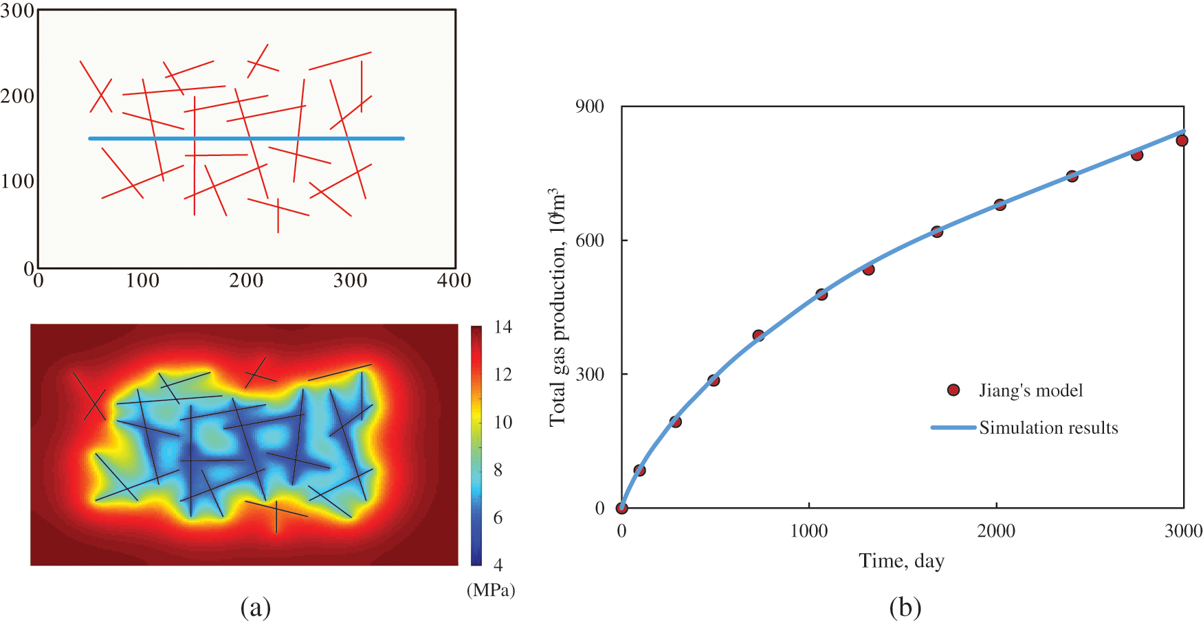
Figure 3: Model validation for a reservoir with a complex fractured well: (a) Horizontal well model and pressure distribution after 3000 days of production; and (b) comparison of the total gas production of our model and Jiang’s model
After 3000 days of production, the pressure drop around the hydraulic fractures was greater, and the range of the pressure drop in the reservoir was closely related to the fracture distribution characteristics. Regarding the total gas production, the results obtained using our model match Jiang’s model well (Fig. 3b).
4.2 Influence of Fracture Network
For a fractured horizontal well with a complex fracture network in a shale gas reservoir block in Southern Sichuan (Fig. 1), the entire region was discretized using structural grids. A fully implicit numerical simulation program was compiled to simulate and predict the production performance characteristics of the fractured horizontal wells. The basic parameters of the model are presented in Table 1.
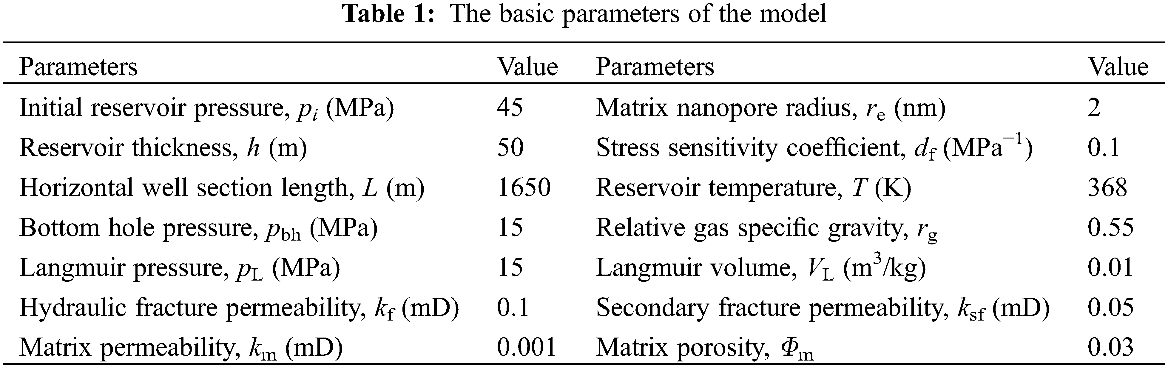
Fig. 4 shows the distribution of the reservoir pressure after one year, five years, and ten years of production from a shale gas fractured horizontal well with a complex fracture network. It can be seen that the range and degree of the reservoir pressure drop are closely related to the shape of the fracture network, and the pressure drop is characterized by a non-uniform distribution. Due to the strong conductivity of the fractures, the pressure drop is the largest around the fracture. The denser the fracture distribution is, the greater the pressure drop is. Because the shale reservoir is relatively tight, the pressure wave propagates slowly in the reservoir, and the swept range is small. This demonstrates that the complex fracture network stimulation area is the main area contributing to the pressure drop and production of the shale gas well. The stimulation of shale reservoirs should be as high as possible within the economic scope to form a complex fracture network around the wellbore.
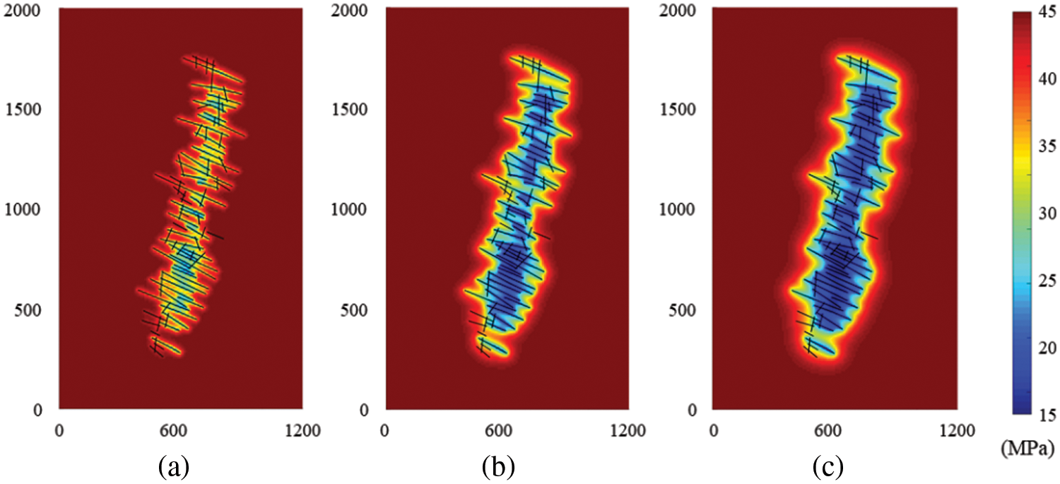
Figure 4: Pressure distribution of a shale gas fractured well with a complex fracture network after (a) 1 year; (b) 5 years; and (c) 10 years of production
4.3 Influence of Micro-Scale Flow Mechanisms
Fig. 5 shows the effect of the micro-scale flow mechanisms on gas production. It can be seen that the cumulative gas production of the fractured horizontal wells after ten years of production without considering the mechanisms is 1.23 × 10⁸ m3, while the cumulative gas production considering the mechanisms is 1.47 × 10⁸ m3. The difference between these two scenarios is 19.5%. If the mechanisms are not considered, the gas production capacity of the gas wells will be underestimated, especially in the later stage of production, which is characterized by prominent adsorption and desorption contributions.
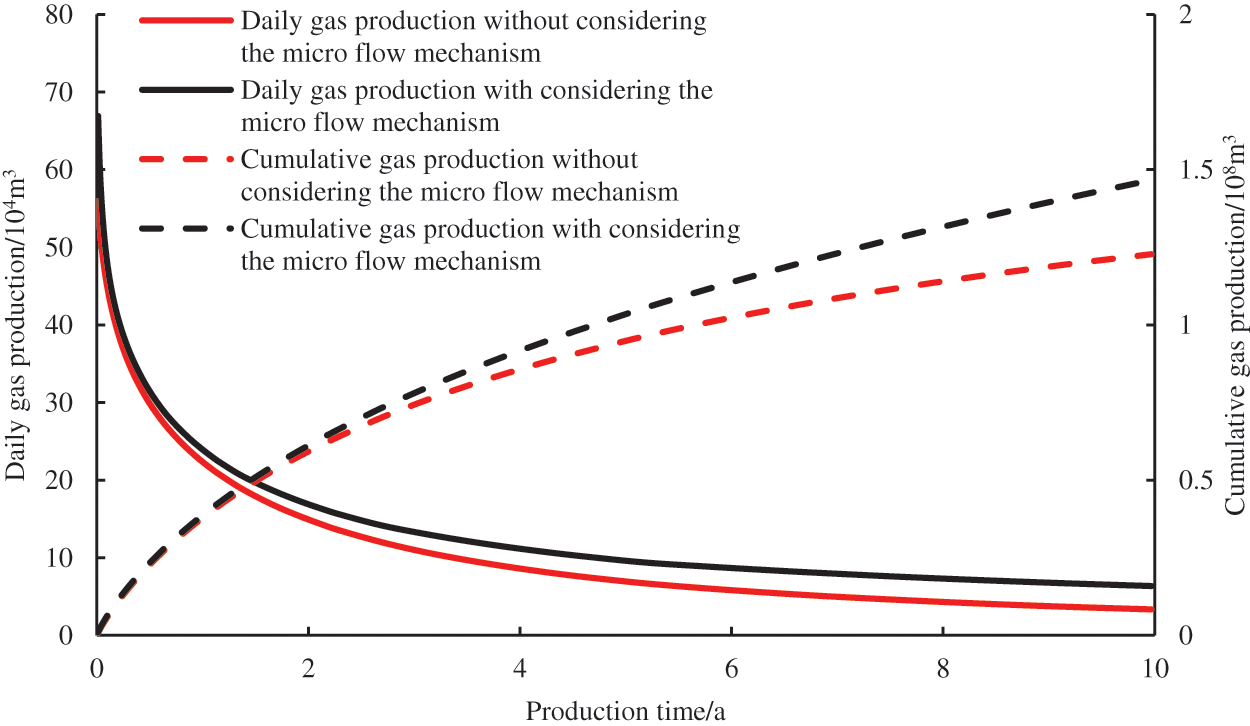
Figure 5: Influence of micro-scale flow mechanisms on gas well production performance
4.4 Influence of Hydraulic Fracture Conductivity
Fig. 6 shows the effect of the hydraulic fracture conductivity on well production. It can be seen from Fig. 6 that the fracture conductivity has a notable impact on the early production of the fractured horizontal wells. The greater the conductivity is, the higher the early daily gas production is, but the difference gradually decreases with increasing production time. When the conductivity CFD is set to 0.1, 0.5, and 1.0 D·cm, the cumulative gas production after ten years is 0.91 × 10⁸ m3, 1.34 × 10⁸ m3, and 1.71 × 10⁸ m3, respectively. Therefore, in hydraulic fracturing in shale gas reservoirs, the conductivity of the hydraulic fractures should be improved as much as possible, thereby increasing production.
Figure 6: Effect of fracture conductivity on gas production
4.5 Influence of the Langmuir Volume
Fig. 7 shows the effect of the Langmuir volume VL on gas production. It can be seen from Fig. 7 that the larger VL is, the larger the daily gas production and cumulative gas production of the gas well are, the slower the rate of decrease of the gas well production is, and the longer it takes for the gas well to reach the stable production stage. As the gas well production progresses, the free gas from the fracture system is preferentially produced. The continuous reduction of the reservoir pressure causes the gas adsorbed on the surfaces of the organic matter to begin to desorb and enter the fracture system as a supplementary gas source in the reservoir, delaying the decrease in the gas well production. When the Langmuir volume VL is set to 0.01, 0.02, and 0.04 m3/kg, the cumulative gas production after ten years of depletion production is 1.01 × 10⁸ m3, 1.35 × 10⁸ m3, and 1.59 × 10⁸ m3, respectively. Adsorption and desorption are important seepage mechanisms that distinguish shale gas reservoirs from conventional gas reservoirs. As production progresses, the reservoir pressure decreases and a large amount of adsorbed gas is desorbed, which helps stabilize the production of the fractured horizontal wells in shale gas reservoirs.
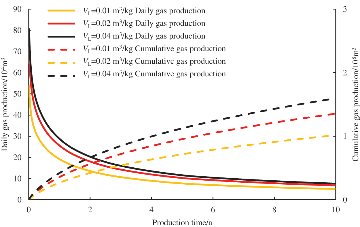
Figure 7: Effects of Langmuir volumes on gas production
4.6 Influence of Bottom Hole Pressure
Fig. 8 shows the influence of the bottom hole pressure on the production of the gas wells. It can be seen that the lower the bottom hole pressure is, the greater the initial daily gas production is, but the increment of the cumulative gas production gradually decreases as the bottom hole pressure decreases. When the bottom hole pressure decreases from 15 to 12 MPa and then to 10 MPa, the cumulative gas production after ten years increases from 1.43 × 10⁸ m3 to 1.66 × 10⁸ m3 and then to 1.81×10⁸ m3. Therefore, reasonable bottom-hole flow pressure should be selected to achieve better production from a fractured well.
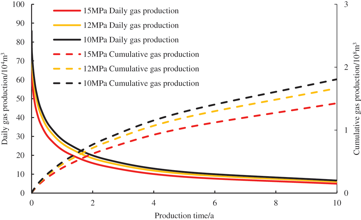
Figure 8: Effects of bottom hole pressure on gas production
(1)A micro-seismic cloud map was used to characterize the hydraulic fracture networks, which can more accurately describe the effective stimulation region after the fracturing of horizontal wells in shale gas reservoirs. Consequently, a more accurate simulation of the production performance of the fractured horizontal wells in shale gas reservoirs can be achieved.
(2)The sensitivity analysis of the parameters revealed that ignoring the microscopic seepage mechanisms will lead to underestimation of the production of the horizontal well. The hydraulic fracture conductivity has a significant impact on the early production of fractured horizontal wells. The larger the Langmuir volume is, the higher the daily and cumulative production are. The lower the bottom hole pressure is, the greater the initial daily gas production is, but the increment of the cumulative gas production gradually decreases as the bottom hole pressure decreases.
(3)For fractured horizontal wells in shale gas reservoirs, the shape of the fracture network significantly affects the pressure drop characteristics. The pressure drop in the reservoir mainly occurs around the hydraulic fractures. it is difficult for the pressure drop to propagate into the reservoir matrix area that is far away from the fractured wells. This is one of the main reasons for the rapid reduction in shale gas well production. Therefore, it is necessary to enlarge the volume of the stimulated reservoir to obtain higher production.
Funding Statement: This work was supported by the National Natural Science Foundation of China (Grant No. 52004237), Science and Technology Cooperation Project of the CNPC-SWPU Innovation Alliance (Grant No. 2020CX020202), and the Sichuan Science and Technology Program (No. 2022JDJQ0009).
Conflicts of Interest: The authors declare that they have no conflicts of interest to report regarding the present study.
References
1. Hamza, A., Hussein, I. A., Al-Marri, M. J., Mahmoud, M., Shawabken, R. et al. (2020). CO2 enhanced gas recovery and sequestration in depleted gas reservoirs: A review. Journal of Petroleum Science and Engineering, 196, 107685. [Google Scholar]
2. Wu, Y. S., Moridis, G. J., Bai, B., Zhang, K. (2009). A multi-continuum model for gas production in tight fractured reservoirs. Paper SPE 118944, pp. 19–21. SPE Hydraulic Fracturing Technology Conference, The Woodlands, Texas, USA. [Google Scholar]
3. Kulga, B., Ertekin, T. (2018). Numerical representation of multi-component gas flow in stimulated shale reservoirs. Journal of Natural Gas Science & Engineering, 56, 579–592. [Google Scholar]
4. Liu, Y. W., Gao, D. P., Li, Q., Wan, Y. Z., Duan, W. J. et al. (2019). Some frontier problems of mechanics in shale gas exploitation. Advances in Mechanics, 49, 1–236. [Google Scholar]
5. Xie, J. (2018). Construction practice and effect of Changning-Weiyuan national-level shale gas demonstration zone. Natural Gas Industry, 38(2), 1–7. [Google Scholar]
6. Fiallos, M., Morales, A., Yu, W. (2018). Characterization of complex hydraulic fractures in Eagle Ford shale oil development through embedded discrete fracture modeling. Petroleum Exploration and Development, 48(3), 613–619. [Google Scholar]
7. Bruno, J., Sun, H., Yu, W. (2021). New diagnostic fracture injection test model with complex natural fractures using embedded discrete fracture model. 55th U.S. Rock Mechanics/Geomechanics Symposium, Virtual. ARMA-2021-1387. [Google Scholar]
8. Xu, Y., Cavalcantefilho, J. S., Yu, W. (2017). Discrete-fracture modeling of complex hydraulic-fracture geometries in reservoir simulators. SPE Reservoir Evaluation & Engineering, 20(2), 403–422. https://doi.org/10.2118/183647-PA [Google Scholar] [CrossRef]
9. Wei, Y. S., Wang, J. L., Yu, W. (2021). A smart productivity evaluation method for shale gas wells based on 3D fractal fracture network model. Petroleum Exploration and Development, 48(4), 787–796. https://doi.org/10.1016/S1876-3804(21)60076-9 [Google Scholar] [CrossRef]
10. Yu, W., Wu, K., Liu, M. L. (2018). Production forecasting for shale gas reservoirs with nanopores and complex fracture geometries using an innovative non-intrusive EDFM method. SPE Annual Technical Conference and Exhibition, Dallas. SPE-191666-MS. [Google Scholar]
11. Ozkan, E., Brown, M., Raghavan, R., Kazemi, H. (2011). Comparison of fractured-horizontal-well performance in tight sand and shale reservoirs. SPE Reservoir Evaluation & Engineering, 14(2), 248–259. https://doi.org/10.2118/121290-PA [Google Scholar] [CrossRef]
12. Stalgorova, E., Mattar, L. (2013). Analytical model for unconventional multifractured composite systems. SPE Reservoir Evaluation & Engineering, 16(3), 246–256. https://doi.org/10.2118/162516-PA [Google Scholar] [CrossRef]
13. Stalgorova, E., Mattar, L. (2012). Practical analytical model to simulate production of horizontal wells with branch fractures. Paper SPE 162515, SPE Canadian Unconventional Resources Conference, Calgray, Alberta, Canada. [Google Scholar]
14. Zhou, W. T., Banerjee, R., Poe, B. D., Spath, J., Thambynayagam, M. (2012). Semi-analytical production simulation of complex hydraulic fracture networks. Paper SPE 157367, SPE International Production and Operations Conference, Doha Qatar. [Google Scholar]
15. Zhao, Y. L., Zhang, L. H., Shan, B. C. (2018). Mathematical model of fractured horizontal well in shale gas reservoir with rectangular stimulated reservoir volume. Journal of Natural Gas Science and Engineering, 59(1), 67–79. https://doi.org/10.1016/j.jngse.2018.08.018 [Google Scholar] [CrossRef]
16. Cusini, M., White, J., Castelletto, N., Settgast, R. (2021). Simulation of coupled multiphase flow and geomechanics in porous media with embedded discrete fractures. International Journal for Numerical and Analytical Methods in Geomechanics, 45(5), 1–22. https://doi.org/10.1002/nag.3168 [Google Scholar] [CrossRef]
17. Odseater, L. H., Kvamsdal, T., Larson, M. G. (2019). A simple embedded discrete fracture-matrix model for a coupled flow and transport problem in porous media. Computer Methods in Applied Mechanics and Engineering, 343(5), 572–601. https://doi.org/10.1016/j.cma.2018.09.003 [Google Scholar] [CrossRef]
18. Jiang, J. M., Rami, M. Y. (2015). A multimechanistic multicontinuum model for simulating shale gas reservoir with complex fractured system. Fuel, 161(1), 333–344. https://doi.org/10.1016/j.fuel.2015.08.069 [Google Scholar] [CrossRef]
19. Xu, Y. F., Cavalcante Filho, J. S. A., Yu, W., Kamy, S. (2017). Discrete-fracture modeling of complex hydraulic-fracture geometries in reservoir simulators. SPE Reservoir Evaluation & Engineering, 20(2), 403–422. https://doi.org/10.2118/183647-PA [Google Scholar] [CrossRef]
20. Altwaijri, M., Xia, Z. H., Yu, W., Qu, L. C., Hu, Y. P. et al. (2018). Numerical study of complex fracture geometry effect on two-phase performance of shale gas wells using the fast EDFM method. Journal of Petroleum Science and Engineering, 164(5), 603–622. https://doi.org/10.1016/j.petrol.2017.12.086 [Google Scholar] [CrossRef]
21. Mayerhofer, M. J., Stegent, N. A., Barth, J. O., Ryan, K. M. (2011). Integrating fracture diagnostics and engineering data in the Marcellus Shale. Paper SPE 145463, SPE Annual Technical Conference and Exhibition, Denver, Colorado, USA. [Google Scholar]
22. Zhao, J. Z., Ren, L., Shen, C. (2018). New progress in research on fracture network fracturing theory and technology in shale gas reservoirs. Natural Gas Industry, 38(3), 1–14. [Google Scholar]
23. Cheng, L. S., Wu, Y. H., Huang, S. J. (2020). A comprehensive model for simulating gas flow in shale formation with complex fracture networks and multiple nonlinearities. Journal of Petroleum Science and Engineering, 187(6), 1–17. https://doi.org/10.1016/j.petrol.2019.106817 [Google Scholar] [CrossRef]
24. Cai, J. C., Lin, D. L., Singh, H. (2018). Shale gas transport model in 3D fractal porous media with variable pore sizes. Marine and Petroleum Geology, 98, 437–447. https://doi.org/10.1016/j.marpetgeo.2018.08.040 [Google Scholar] [CrossRef]
25. Cheng, S. X., Huang, P., Wang, K. (2020). Comprehensive modeling of multiple transport mechanisms in shale gas reservoir production. Fuel, 277(3), 118159. https://doi.org/10.1016/j.fuel.2020.118159 [Google Scholar] [CrossRef]
26. Wu, K. L., Li, X. F., Chen, Z. X. (2016). Microscale effect of gas transport in shale gas organic matter nanopores. Natural Gas Industry, 36(11), 51–64. [Google Scholar]
27. Javadpour, F., Fisher, D., Unsworth, M. (2007). Nanoscale gas flow in shale gas sediments. Journal Gas of Canadina Petroleum Technology, 46(10), 55–61. https://doi.org/10.2118/07-10-06 [Google Scholar] [CrossRef]
28. Jiang, J., Rami, M. (2015). A generic physics-based numerical platform with hybrid fracture modelling techniques for simulating unconventional gas reservoirs. Paper SPE-173318-MS, SPE Reservoir Simulation Symposium, Houston, Texas, USA. [Google Scholar]
Cite This Article
 Copyright © 2023 The Author(s). Published by Tech Science Press.
This work is licensed under a Creative Commons Attribution 4.0 International License , which permits unrestricted use, distribution, and reproduction in any medium, provided the original work is properly cited.
 Downloads
 Citation Tools