
 Submit a Paper
 Propose a Special lssue
 Open Access
ARTICLE

Computation of Stiffness and Damping Derivatives of an Ogive in a Limiting Case of Mach Number and Specific Heat Ratio
1
Department of Mathematics, Mangalore Institute of Technology and Engineering, Moodabidri, 574225, India
2
Department of Mathematics, Sahyadri College of Engineering & Management, Mangalore, 575007, India
3
Department of Mechanical and Aerospace Engineering, Faculty of Engineering, International Islamic University, Kuala Lumpur,
53100, Malaysia
4
Department of Engineering Management, College of Engineering, Prince Sultan University, Riyadh, 11586, Saudi Arabia
* Corresponding Author: Aysha Shabana. Email:
Fluid Dynamics & Materials Processing 2023, 19(5), 1249-1267. https://doi.org/10.32604/fdmp.2023.023158
Received 12 April 2022; Accepted 11 August 2022; Issue published 30 November 2022
 View Full Text
 Download PDF
Abstract
This work aims to compute stability derivatives in the Newtonian limit in pitch when the Mach number tends to infinity. In such conditions, these stability derivatives depend on the Ogive’s shape and not the Mach number. Generally, the Mach number independence principle becomes effective from M = 10 and above. The Ogive nose is obtained through a circular arc on the cone surface. Accordingly, the following arc slopes are considered λ = 5, 10, 15, −5, −10, and −15. It is found that the stability derivatives decrease due to the growth in λ from 5 to 15 and vice versa. For λ = 5 and 10, the damping derivative declines with an increase in λ from 5 to 10. Yet, for the damping derivatives, the minimum location remains at a pivot position, h = 0.75 for large values of λ. Hence, when λ = −15, the damping derivatives are independent of the cone angles for most pivot positions except in the early twenty percent of the leading edge.Keywords
The analysis of supersonic/hypersonic of simple shapes like wedges, cones, and Ogives are of great interest when oscillating at high Mach numbers, and significant incidences are of great interest. Researchers have shown great interest owing to the advent of the space program and high-speed fighter aircraft because of the cost involved in conducting experiments at high Mach numbers. Therefore, simple but reasonably accurate techniques are needed to compute the aerodynamic load and stability derivatives during re-entry. And more so, such parametric computations are very valuable in the initial design process when various geometrical and inertia parameters are investigated.
The present work aims to evaluate pitch aerodynamic stiffness and damping derivatives for limiting cases. In this situation, flow parameters are not dependent on the inertia levels. However, flow parameters are a function of geometry. In the Newtonian limit, Mach numbers will tend to infinity. The specific heat ratio (γ) at constant pressure and volume, with a constant value of 1.4 (i.e., γ = 1.4) at a standard ballistic atmosphere, becomes unity. The knowledge of aerodynamic derivatives at the Newtonian limit can be handy for the space program. For launch vehicles, the flow Mach number becomes very high. In aerodynamic vehicles like hypersonic missiles and the space shuttle, the focus of study shifts from optimizing the aerodynamic shapes to reduce the drag force to focusing on aerodynamic heating. At supersonic flow, the primary concern is to minimize the drag of the projectiles and missiles. The easiest option is to have a blunt nose instead of a sharp nose, which will give immediate relief from the high-temperature build-up at the nose. Unique material is used for the nose portion of the hypersonic missiles and the aircraft to address the issue of high temperature at the design stage. For space shuttles, tiles are used to protect from aerodynamic heating.
Appleton [1] evaluated stiffness and damping derivatives in pitch for a wedge in hypersonic flow. Brong [2] and Ericsson [3] studied the flow field of the right circular cone in unsteady flight. The large deflection hypersonic similitude of Ghosh [4] was applied by Ghosh et al. [5]. They devised another hypersonic similarity for the attached shock case. The Mach after the shock must be more than 2.5 (i.e., M2 > 2.5). He ignored the impact of the Lee surface as the contribution from the Lee surface was negligible. He mainly focussed on the windward side accompanied by an oblique shock wave at the plate. A unified supersonic/hypersonic theory for delta wings and cones was developed by Ghosh [6,7]. Hui [8,9] studied oscillating wedges and caret wings to evaluate supersonic/hypersonic flow stability derivatives. Hui et al. [10,11] used the unsteady Newton-Buseman theory. The role of dynamic during re-entry or maneuver was discussed by Orlik-Ruckman [12–14]. Shabana et al. [15,16] computed the stability derivatives for supersonic/hypersonic flow cones. They used these theories, resulting in the Newtonian limit and a fixed specific heat ratio. Monis et al. [17] studied the effect of secondary wave reflections on supersonic/hypersonic flow wings. Crasta et al. [18] estimated the surface pressure distribution on a delta wing with curved leading edges in hypersonic/supersonic flow using mathematical modelling and results shows impact on finding the pressure distribution over an delta wing. Later on, softcomputing approach was found via computational fluid dynamics (CFD) method and Khan et al. [19–21] computed the flow field around the 2-D wedge. Interestingly, the study of high-speed flow was limited to a slim body, and small angles of incidence are extended for high angles of attack.
An axisymmetric Ogive is obtained by the revolution of the plane Ogive of semi-nose angle δ =
Figure 1: Geometry of cone and Ogive
As the Ogive move with a velocity of
where
The projection of point A (Fig. 1) on the axis of symmetry has a distance of x, and the pivot point 01 has a length of xo from the apex.
Let α be the pitch angle at any instant, and q be the pitch rate. Therefore, the local piston Mach number at A is
If Ψ is the azimuthal angle (Fig. 1) subtended by a tiny area element at B, then
After simplification, we obtain
In the limit α, q →0,
where
Hence
Putting
Differentiating Eq. (9), concerning
And from Eq. (1),
Since
where
where
Expanding Binomially, and neglecting higher-order terms and simplifying, we obtain
On simplification, we get
where
Further simplifying, we obtain
and
Now expanding Eq. (12), we get
This expression must be evaluated in the limit
Hence, from Eqs. (10), (13), (24), and (25) we have
And
Therefore
After simplification, we obtain
where
From Fig. 1, we have
where
Hence
where
Substituting Eq. (35) in Eq. (5) and dropping the subscript B; subsequently, we have the local piston Mach number as
Hence
And
The expression for the total pitching moment of the Ogive is given by
Here Pb is given by Eq. (1).
The stiffness derivative,
where
Sb = Ogive surface area =
c = chord size of an Ogive
Since Pb is a function of Mp,
Substituting from Eq. (41)
where
Now, substituting for
Putting
where
Since
and
Putting
Substituting I1 and I2 in Eq. (21)
Substituting Eq. (24) in (20) and putting back the values of
Hence on simplification, we obtain
where
The Damping derivative
where
On solving similarly like above, we obtain
where
and
For limiting case
By applying limit
where
Therefore, the Stiffness derivative in the limiting case is given by
Hence, the Damping derivative in the limiting case is given by
The results were computed and discussed based on the stiffness and damping derivatives formulations. Before analyzing the results, we must keep in mind that we evaluate stiffness & damping derivatives for a limiting case where M tends to infinity. The value of γ of air is typically 1.4, but it will increase to unity in the Newtonian limit. The following parameter is the very high Mach number. Because Mach becomes infinity, which implies that Mach number will no more be a variable, outcomes will indicate the impact of the geometric constraints alone in the present case. We are considering these circumstances while discussing the results.
Fig. 2 demonstrates the reliance of stiffness pitch derivative with h for numerous angles from 10° to 25° and Ogive slope λ. The stiffness derivative’s linear growth is due to the rise in cone angle. When there is a rise in the cone angle, the surface area will increase, hence the surface pressure variation. Stiffness derivative attains maximum values at h = 0. The reason for this high value is the maximum pitching moment arm. The position of the resultant force has shifted in the direction of flow. It remains from h = 0.6 to 0.8 for cone angles from ten to twenty-five degrees. That indicates that the cones with higher angles will be more stable than those with small angles due to the swing of the resultant force in the flow direction.
Figure 2: Variation of Stiffness Derivatives vs. Pivot position (h)
Results for cone angles from 10 to 25 degrees & λ = −5 are shown in Fig. 3. Since λ = −5, it is convex in shape and will have a different surface distribution. When λ = 5, it is concave and shifts the larger area of the cone towards the trailing edge resulting in a stable aerospace vehicle. A peculiar trend is seen in this case’s results and flow field. The stability derivatives assume higher values than the higher cone angles, and the tendency reverses at h = 0.4. The center of pressure moved towards the flow direction, but it remained in h = 0.75 to 0.85. The higher values of stability derivatives are seen in the latter part of the cone due to the edge pressure distribution.
Figure 3: Variation of Stiffness Derivatives vs. Pivot position (h)
When the Ogive arc λ = 10 and other parameters are the same, the outcomes of the stiffness derivatives are displayed in Fig. 4. It indicates a severe decrement in the stiffness derivatives and location of net force found from h = 0.52 to 0.75. However, there is a gradual rise in the stiffness derivatives, as seen earlier. This trend may be due to the high Ogive arc; the surface area of the Ogives is decreased significantly, resulting in decreased values.

Figure 4: Variation of Stiffness Derivatives vs. Pivot position (h)
Fig. 5 indicates the variation of stiffness derivatives with h. With an increase in the Ogive slope from λ = −5 to −10. This change in λ will affect a further variation in the edge of the Ogive and modification in the pressure dispersal of the surface and hence the stiffness stability derivative. The pattern is similar as was seen for λ = −5, with considerable growth in the amount of the stiffness derivatives. The location center of the pressure band has been narrowed down and further moved towards the flow direction. In this case, it remains from h = 0.78 to h = 0.87. This shift is attributed to the increased arc Ogive radius.

Figure 5: Variation of Stiffness Derivatives vs. Pivot position (h)
Fig. 6 represents the outcomes for Ogive arc λ = 15 for the same cone angles from 10 to 25 degrees. Results show a further decrease of the stiffness derivatives due to the Ogive slope change, resulting in a further reduction in the surface area. The figure shows considerable change in the center of pressure location as the arch of the Ogive will form a concave surface and shift the significant area of the Ogive surface towards the trailing edge. The center of pressure varies in the band of h = 0.35 to 0.72. That shows that the stiffness derivatives take a meager value for lower cone angles. Significant movement of the net force in the flow direction results in a tiny moment arm, resulting in a low static margin, and it is undesirable. However, for a cone angle of twenty-five degrees, there is a significant shift in the center of pressure, causing a large moment arm and higher values of the static margin.

Figure 6: Variation of Stiffness Derivatives vs. Pivot position (h)
Fig. 7 depicts the results for λ = −15, resulting in an increased surface of the Ogive for cone angles from 10 to 25 degrees. The magnitude of the increase in λ from −10 to −15 has increased significantly, hence the larger stiffness derivatives values. The movement of the center of pressure is limited to h = 0.8 to 0.86. Stiffness derivative declines with a rise in the cone angle. However, this trend gets reversed at h = 0.6. This reversal was happening at h = 0.4 for λ = −5. One of the greatest advantages here is the center of pressure location at h = 0.8 to 0.88. Here is a significant growth of stiffness derivative and the position of the center of pressure, which has also significantly shifted in the flow direction. This increase will lead to a significant increase in the static margin.

Figure 7: Variation of Stiffness Derivatives vs. Pivot position (h)
Fig. 8 shows damping derivatives concerning pitch rate q for a quasi-steady Ogive with λ = 5 for 10 to 25 cone angles. Results show a sudden increase in the damping derivatives and a decrease continuously with the pivot position h. As we move downstream, a reversal in the trend occurs at h = 0.8, which seems to be the center of pressure. This behavior reiterates that the surface area swing towards the trailing edge is due to the surface area. Results suggest the center of pressure is located at twenty percent from the leading edge, which will result in a substantial increase in the damping derivatives, making the system more stable. Any disturbance from the air current or gust to the system can dampen out quickly and bring the system back to a steady state.
Figure 8: Variation of Damping Derivatives vs. Pivot position (h)
Results for λ = −5 are seen in Fig. 9, and the cone angle remains in the same range as discussed earlier. The figure shows that the pattern for this case is different compared to when λ = 5. When λ is positive, the surface is concave, whereas, for λ negative, it is convex. This change in the Ogive nose will result in an enormous variation in the surface pressure distribution, and this variation in pressure is responsible for the difference in the damping derivatives. For this case, damping derivatives take higher values; however, the results are identical for cone angles from 10 to 15 degrees. A minimal rise in the numerical estimates of the damping derivatives is noticed for cone angles 20 and 25 degrees. It maintains a reversal of the trends at h = 0.8. Cone angles within the 20 to 25 degrees range are optimum for this case. However, there is no meaningful change in the damping derivatives for cone angle at 10 to 15 degrees, even though the center of pressure has moved far downstream, resulting in a dynamically stable system.
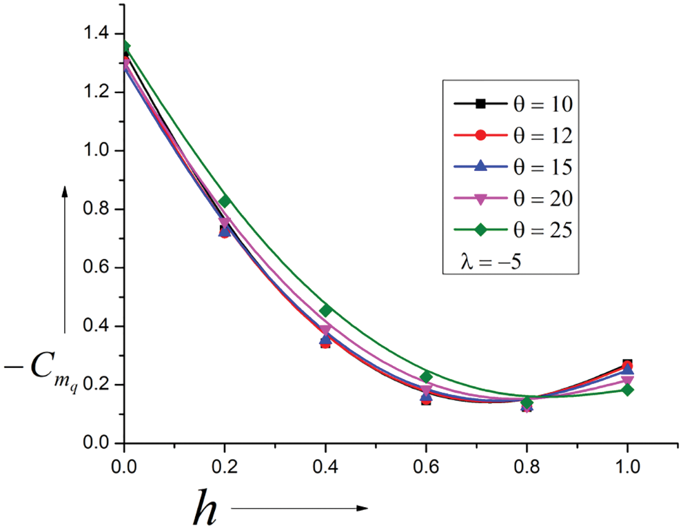
Figure 9: Variation of Damping Derivatives vs. Pivot position (h)
When λ = 10, the outcomes of the present investigations are shown in Fig. 10. An increase in λ = 5 to 10 indicates a considerable decrease in the surface area. That has directly affected the magnitude of the damping derivatives. There is a shift in the reversal trend towards the leading edge at h = 0.72. Otherwise, the trends are similar to lower values of the λ = 5. The damping derivative decreases from h = 0 to h = 0.72, attains minima, and starts increasing again. Here is a substantial decline in damping values from the dynamic stability considerations. The figure shows that the decrease in the damping derivative is around fifty percent. Hence the Ogive with λ = 10 is not the best option considering pitch stability.
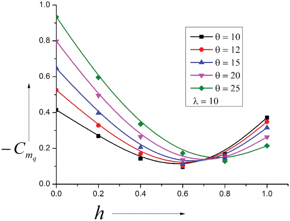
Figure 10: Variation of Damping Derivatives vs. Pivot position (h)
When λ = −10, the discrepancy of the damping derivatives with the pivot position is shown in Fig. 11 for the same range of the cone angles. Due to an increase in the λ = −5 to −10. The magnitudes of the damping derivatives are increased significantly for cone angles from 10 to 20 degrees. Negligible variation is seen in the values for the highest cone angle of 25 degrees. The trend reversal has moved in the flow direction at h = 0.9. Hence, the damping derivative will increase considerably as the center of pressure shifts in the flow direction, leading to larger values of the stability derivatives and, consequently, a dynamically stable system.

Figure 11: Variation of Damping Derivatives vs. Pivot position (h)
Results for λ = 15 are shown in Fig. 12 for cone angles ranging from 10 to 25 degrees. It is seen that when λ = 15, the Ogive form is such that the surface pressure allocation has augmented significantly, resulting in a changed pattern for lower cone angles, mainly ten degrees. Hence, if λ = 15 is used, it is better to avoid ten and twelve degrees cone angles to have similar results. The reversal’s location in the results’ outline has shifted at h = 0.75. The magnitude of the damping derivatives is minimal, owing to a reduction in Ogive area. For this combination of the parameters, cone angles of 15 to 25 degrees are a better option.

Figure 12: Variation of Damping Derivatives vs. Pivot position (h)
When λ = −15, damping derivatives for similar cone angles, as discussed earlier in Fig. 13. The figure shows that cone angles do not influence the damping derivatives as the shape of the surface is convex. Only a marginal impact is seen for a cone angle of twenty-five degrees. Hence, based on the experience gained, it can be stated that when λ = −15, damping derivatives are independent of the cone angles for most of the pivot position except in the early twenty percent of the leading edge.
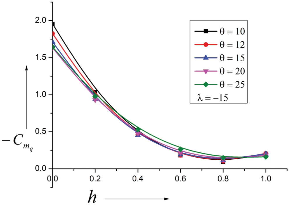
Figure 13: Variation of Damping Derivatives vs. Pivot position (h)
Because of the above deliberations, we may conclude our discussion as under:
• The linear growth in the stiffness derivative is seen owing to the cone angle growth. With the rise in the Ogive slope from λ = 5 to 10, linear decrease in the stiffness derivative are seen, and it attains maximum values at h = 0, and the center of pressure is from h = 0.65 to 0.8 λ = 5 & from h = 0.52 to 0.75 for λ = 10.
• For λ = 15, it is seen that the contour of the Ogive is such that the surface pressure allocation has augmented significantly. Hence, if λ = 15 is used, avoiding cone angles ten and twelve degrees is better. The reversal’s location in the results’ outline has shifted at h = 0.75. For this combination of the parameters, cone angles of 15 to 25 degrees are a better option.
• A peculiar trend is seen in the results and the flow field for this case for λ = −5. The stability derivatives assume higher values than the higher cone angles, and the tendency reverses at h = 0.4. Based on the results obtained, it is recommended that cones with λ = −5 need not consider for design.
• For λ = −15, it increases the Ogive surface for cone angles from 10 to 25 degrees. The magnitude of the increase in λ from −10 to −15 has increased significantly, hence the larger stiffness derivatives values. The variation of the center of pressure is limited to the range from h = 0.8 to 0. 86.
• For λ = 5 and 10, the damping derivative declines with an increase in λ from 5 to 10. The location of minima remains at h = 0.75, which is also the center of pressure. For λ = 15, the form of Ogive is such the surface pressure distribution has augmented significantly, resulting in a changed pattern for lower cone angles, mainly ten degrees. Hence, avoiding cone angles ten and twelve degrees is better to have similar results. For this combination of the parameters, cone angles of 15 to 25 degrees are a better option.
• When λ = −5, −10, and −15, there is a progressive increase in the stiffness cone angles that do not influence the damping derivatives as the shape of the surface is convex. Only a marginal impact is seen for a cone angle of twenty-five degrees. Hence, it can be stated that when λ = −15, damping derivatives are independent of the cone angles for most of the pivot places except in the early twenty percent of the leading edge.
• The current theory for oscillating cones is limited to the quasi-steady case: the primary issue in considering the unsteady case would be the flow being non-uniform in the conical-annular space, even for the steady piston. The Mach waves’ velocity is variable, contrasting the waves in front of a plane piston equivalent to the oscillating wedge.
Acknowledgement: This research is supported by the Structures and Materials (S&M) Research Lab of Prince Sultan University. Furthermore, the authors acknowledge Prince Sultan University’s support for paying this publication’s article processing charges (APC).
Funding Statement: The authors received no specific funding for this study.
Conflicts of Interest: The authors declare they have no conflicts of interest to report regarding the present study.
References
1. Appleton, J. P. (1964). Aerodynamic pitching derivatives of a wedge in hypersonic flow. AIAA Journal, 2(11), 2034–2036. DOI 10.2514/3.2729. [Google Scholar] [CrossRef]
2. Brong, E. (1965). The flow field about a right circular cone in unsteady flight. 2nd Annual Meeting, San Francisco, CA, USA. [Google Scholar]
3. Erisson, L. E. (1973). Unsteady embedded Newtonian flow. Astronautica Acta, 18(5), 309–330. [Google Scholar]
4. Ghosh, K. (1977). A new similitude for aerofoils in hypersonic flow. Proceedings of the 6th Canadian Congress of Applied Mechanics, pp. 685–686. Vancouver, Canada. [Google Scholar]
5. Ghosh, K., Mistry, B. K. (1980). Large incidence hypersonic similitude and oscillating nonplanar wedges. AIAA Journal, 18(8), 1004–1006. DOI 10.2514/3.7702. [Google Scholar] [CrossRef]
6. Ghosh, K. (1984). Hypersonic large-deflection similitude for quasi-wedges and quasi-cones. The Aeronautical Journal, 88(873), 70–76. [Google Scholar]
7. Ghosh, K. (1984). Hypersonic large deflection similitude for oscillating delta wings. The Aeronautical Journal, 88(878), 357–361. [Google Scholar]
8. Hui, W. H. (1969). Stability of oscillating wedges and caret wings in hypersonic and supersonic flows. AIAA Journal, 7(8), 1524–1530. DOI 10.2514/3.5426. [Google Scholar] [CrossRef]
9. Hui, W. H. (1969). Interaction of a strong shock with Mach waves in unsteady flow. AIAA Journal, Technical Note, 7(8), 1605–1607. DOI 10.2514/3.5441. [Google Scholar] [CrossRef]
10. Hui, W. H., Tobak, M. (1981). Unsteady Newton-Busemann flow theory—Part I: Airfoils. AIAA Journal, 19(3), 311–318. [Google Scholar]
11. Hui, W. H., Tobak, M. (1981). Unsteady Newton-Busemann flow theory—Part II: Bodies of revolution. AIAA Journal, 19(10), 1272–1273. [Google Scholar]
12. Orlik-Rückemann, K. J. (1966). Effect of wave reflections on the unsteady hypersonic flow over a wedge. AIAA Journal, 4(10), 1884–1886. DOI 10.2514/3.3813. [Google Scholar] [CrossRef]
13. Orlik-Rückemann, K. J. (1972). Oscillating slender cone in viscous hypersonic flow. AIAA Journal, 10(9), 1139–1140. DOI 10.2514/3.50335. [Google Scholar] [CrossRef]
14. Orlik-Rückemann, K. J. (1975). Dynamic stability testing of aircraft needs versus capabilities. Progress in the Aerospace Sciences, 16(4), 431–447. DOI 10.1016/0376-0421(75)90005-6. [Google Scholar] [CrossRef]
15. Shabana, A., Monis, R. S., Crasta, A., Khan, S. A. (2018). Computation of stability derivatives of an oscillating cone for specific heat ratio = 1.66. IOP Conference Series: Materials Science and Engineering, 370(1), 012059. DOI 10.1088/1757-899X/370/1/012059. [Google Scholar] [CrossRef]
16. Shabana, A., Monis, R. S., Crasta, A., Khan, S. A. (2018). Estimation of stability derivatives in Newtonian Limit for an oscillating cone. IOP Conference Series: Materials Science and Engineering, 370(1), 012061. DOI 10.1088/1757-899X/370/1/012061. [Google Scholar] [CrossRef]
17. Monis, R. S., Shabana, A., Crasta, A., Khan, S. A. (2019). Effect of sweep angle and a half sine wave on roll damping derivative of a delta wing. International Journal of Recent Technology and Engineering, 8(2S3), 984–989. [Google Scholar]
18. Crasta, A., Pavitra, S., Khan, S. A. (2016). Estimation of surface pressure distribution on a delta wing with curved leading edges in hypersonic/supersonic flow. International Journal of Energy, Environment and Economics, 24(1), 67–73. [Google Scholar]
19. Khan, S. A., Crasta, A. (2010). Oscillating Supersonic delta wings with curved leading edges. Advanced Studies in Contemporary Mathematics, 20(3), 359–372. [Google Scholar]
20. Khan, S. A., Aabid, A., Saleel, C. A. (2019). CFD simulation with analytical and theoretical validation of different flow parameters for the wedge at supersonic mach number. International Journal of Mechanical & Mechatronics Engineering, 19(1), 170–177. [Google Scholar]
21. Khan, S. A., Aabid, A., Mokashi, I., Al-Robaian, A. A., Alsagri, A. S. (2019). Optimization of two-dimensional wedge flow field at supersonic mach number. CFD Letters, 11(5), 80–97. [Google Scholar]
Cite This Article
 Copyright © 2023 The Author(s). Published by Tech Science Press.
This work is licensed under a Creative Commons Attribution 4.0 International License , which permits unrestricted use, distribution, and reproduction in any medium, provided the original work is properly cited.
 Downloads
 Citation Tools