Optimal Structural Parameters for a Plastic Centrifugal Pump Inducer

1  Introduction

Pumps are very widely used general-purpose machines, and they operate almost everywhere there is fluid flow. The inducer belongs to the axial flow impeller, after the rotation of the spiral vanes to do work, so that the energy of the outlet fluid increases, and at the same time play a pre-rotation of the fluid, which does not cause blockage of the entire flow channel [1], the front inducer can generate a certain pressure at the impeller inlet, so that the main impeller can operate under pre-pressure [2].

Wang et al. [3] analyzed and compared the effects of different inducers and their matching relationship with the impeller on the flow field characteristics inside the centrifugal pump; Wu et al. [4] showed that the addition of inducers could significantly reduce the area of the low pressure zone at the back of the vane inlet, and the performance of variable-pitch inducers was better than that of equal-pitch inducers; Shojaeefard et al. [5] used the ratio of inlet vane tip angle, outlet vane tip angle and outlet hub radius The ratio of inlet lobe tip angle, outlet lobe tip angle and outlet hub radius to inlet hub radius were used as design variables, and the hydraulic efficiency and the required net positive suction head (NPSHR) were used as performance indicators of the inducer to investigate how to improve the pump performance. The results showed that the hydraulic efficiency and NPSHR of the pump were improved by 0.3% and 30.2%, respectively. Kang et al. [6] investigated the performance of centrifugal pumps with different number of vanes of inducers and showed that the pump performance was better when the number of inducer vanes was 3. Ito et al. [7] pointed out that the backflow phenomenon in the gap at the top of the inducer impeller was caused by the large pressure difference between the suction and pressure surfaces at the inlet of the vanes. Tani et al. [8] studied the effect of inducer pitch variation on the performance of centrifugal pumps and explained that the leakage flow in the lobe top gap is from the working surface to the back of the inducer.

Cheng et al. [9] investigated the effect of different leading edge wrap angles of inducer blades on the performance of centrifugal pumps and found that the pump head gradually decreased when the leading edge wrap angle increased from 120° to 270°. Sun et al. [10] studied the effect of variable pitch inducer geometry and matching with impeller on the performance of centrifugal pumps. Kang et al. [11] found that a smaller inlet angle of the inducer vane can avoid the instability of cavitation under high flow conditions; Furukawa et al. [12] used experimental studies to obtain the effects of the number of inducer vanes, the consistency of the lobe and the vane angle on its head; Kim et al. [13] used numerical calculations to study the effect of various vane top Cheng et al. [14] used coolant pumps to evaluate the effect of impeller/guide vane clearance (clearance ratio) on the performance of such pumps. The results showed that the effect of clearance ratio on the maximum equivalent force at the back of the impeller vanes was greater than that at the working surface. Parikh et al. [15] used a multi-objective optimization approach to find an optimum geometry of the inducer to ensure efficient operation of the inducer over a relatively wide range of flow rates. The results showed that blade length, blade swept-back angle, tip clearance and blade thickness should be kept low and that the best performance is achieved with an inducer having a high hub taper angle and three blades. Shojaeefard et al. [16] optimized the performance of the inducer using the inlet blade tip angle, outlet blade tip angle and the ratio of outlet hub radius to inlet hub radius as design variables and the head coefficient, hydraulic efficiency and required net positive suction head (NPSHR) as objective functions.

Compared with the above references, this paper mainly uses orthogonal tests and fish swarm algorithms to optimize the structural parameters of the inducer. The orthogonal experiment table of inducer structure L16 (165) is designed, and the five factors of inducer blade thickness S, cascade solidity t, blade rim angle β1, blade hub angle β2, hub length L of plastic centrifugal pump are selected for the orthogonal experiment, and the evaluation indexes are shaft power and head. Through the CFX simulation, the orthogonal experiment is completed and the extreme difference analysis is performed on the orthogonal experiment to obtain the ranking of the influence of each structural parameter on the evaluation indexes in each optimization direction and its influence, and the optimization method based on least squares and fish swarm algorithm is applied to optimize the shaft power and head of the plastic centrifugal pump.

2  Parameter Design of Plastic Centrifugal Pump Model

2.1 Design of Model Pump Parameters

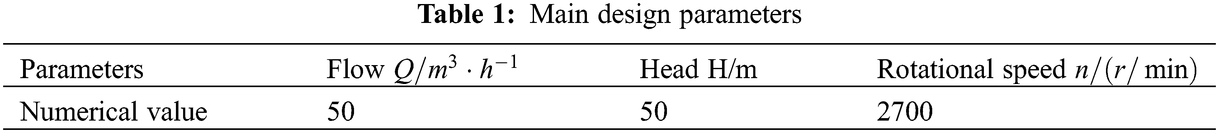
The centrifugal pump studied in this paper is a low specific rpm centrifugal pump, and other main parameters are as follows Table 1.

(1)    The inlet diameter and inlet speed of the pump

Ds=4QπVs (1)

In Eq. (1), the

Ds -Pump inlet diameter (m);

Q -Pump flow rate (m3/h);

Vs -Pump inlet flow rate (m/s);

Take the pump inlet flow rate Vs = 2.73 m/s [1], then the pump inlet diameter Ds = 80 mm.

(2)    Pump outlet diameter and outlet speed

The outlet diameter of the plastic centrifugal pump is calculated according to the following formula:

Dd=(0.7−1)Ds (2)

In Eq. (2), the Dd -Pump outlet diameter (mm).

The contact factor is 0.9, so the pump outlet diameter Dd = 68 mm.

The pump outlet velocity is calculated as follows:

Vd=4QπDd2 (3)

In Eq. (3), the Vd -Pump outlet flow rate m/s.

The calculation gives Vd = 3.826 m/s.

(3)    Specific speed

ns=3.65nQH34 (4)

In Eq. (4), the ns -Ratio speed. H -Head (m).

After calculation, we get: ns = 61.78.

(4)    Hydraulic efficiency of the pump

The hydraulic efficiency of the pump is calculated according to Eq. (5) as follows:

ηh≈1+0.083511gQn3 (5)

Bringing in the data is calculated as ηh = 0.852.

(5)    Volume efficiency of the pump

The volumetric efficiency of the plastic pump is calculated according to Eq. (6)

ηv≈11+0.68ns−23 (6)

Bringing in the data is calculated as ηv = 0.96.

(6)    Mechanical efficiency of the pump

The mechanical efficiency of the disc friction loss is calculated by Eq. (7)

ηm≈1−0.07(ns100)76 (7)

Bringing in the data is calculated as ηm = 0.88.

(7)    Total efficiency of the pump

The total efficiency of the plastic pump is calculated according to Eq. (8)

η=ηhηvηm (8)

Bringing in the data is calculated as η = 0.72.

Plastic centrifugal pump head calculation formula.

H=Pout−Pinρg+Δz (9)

In Eq. (9), the

Pout -Total pressure at the volute outlet, Pa. Pin -Total impeller inlet pressure, Pa. Δz -Difference in height between pump inlet and outlet, m. Plastic centrifugal pump shaft power calculation formula.

P=M∗ω (10)

where M is the torque, N⋅m , and ω is the angular velocity, rad/s.

2.2 Determination of the Main Dimensions of the Impeller

The structure form of centrifugal pump impeller is mainly semi-open type and closed type, among which semi-open type impeller has the advantages of high strength and easy molding. Therefore, the impeller used in this paper is semi-open type. The structure of the impeller is shown in Fig. 1.

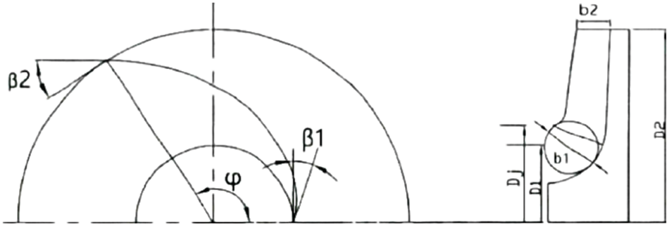
Figure 1: Impeller structure diagram

This paper applies the velocity coefficient method to design and calculate the impeller structural parameters.

(1)    Impeller inlet diameter

Impeller inlet equivalent diameter is calculated according to Eq. (11)

D0=k0Qn3 (11)

In Eq. (12), the k0 -Factor, take k0 = 4.5[1].

Substituting into the above equation gives D0 = 78 mm.

For impeller inlet diameter calculated by Eq. (12).

Dj=D02+dh2 (12)

In Eq. (12), the dh -Wheel diameter (mm);

dh is valid only for structural design, for hydraulic design, dh = 0; then Dj=D0  = 78 mm, take Dj = 80 mm.

The blade inlet diameter is estimated as follows:

D1=k1Dj (13)

In Eq. (13), the k1 -Coefficient, generally taken from k1 = 0.7 to 1.0.

The coefficient k1 , which is determined by the specific speed, is taken as a large value for low specific speed and a small value for high specific speed. According to this paper, the specific speed is taken as k1 = 0.85, then D1 = 68 mm.

(2)    Impeller inlet width

The inlet width of the impeller blade is determined by Eq. (14)

b1=D14k1ξ1 (14)

In Eq. (14), the ξ1 -Ratio of impeller inlet speed to inlet diameter.

Generally take ξ1 = 0.9∼1.0, and substitute D1=115mm,k1 = 0.85 into the Eq. (14) to get b1 = 20 mm.

(3)    Impeller outlet diameter

The blade inlet diameter is first preliminarily estimated

D2=kDQn3 (15)

kD=9.35kD2(ns100)−12 (16)

In Eq. (15), the kD - D2 Correction coefficient.

kD is related to the type and specific speed of the pump, this paper uses a single-stage pump, and the specific speed ns = 61.78, so choose kD2 = 1.038. The calculation results are D2 = 210 mm.

(4)    Impeller outlet width

The blade exit width is calculated by the following two equations:

b2=kbQn3 (17)

kb=0.78kb2(ns100)56 (18)

In Eq. (17), the kb−b2 Correction coefficient.

kb is related to the type and specific speed of the pump, this paper uses a single-stage pump, and the specific speed ns  = 61.78, so kb2  = 1.236 is chosen. Substitute into the calculation to get b2 = 11 mm.

(5)    Number of blades

The number of blades is calculated by Eq. (19)

Z=6.5D2+D1D2−D1sinb1+b22 (19)

The values of D1 , D2 , b1 and b2 are substituted into the calculation; when the impeller diameter is the same, increasing the number of blades will increase the head, but not change its flow rate value, and the integrated given head H = 50 m, so take Z = 6.

(6)    Impeller inlet and outlet placement angle

In this paper, the blade inlet settling angle β1 is 19°, the outlet settling angle is 33°, and the wrap angle φ is 123° [17].

(7)    Blade thickness design

In the design of plastic impeller, the reduction of thickness makes the flow channel wider, the slip coefficient is reduced so that the pump shaft power is increased, but the thickness can not be unlimited small, otherwise because of the lack of strength makes the impeller deformation is too large to work; the same thickness will make the flow channel narrower, the hydraulic loss is increased, so the thickness of the blade in this paper is 2 mm.

2.3 Main Dimensions of the Volute

The overflow parts of the pump include the impeller and the volute, the volute is also one of the overflow parts to convert energy, the main dimensions of the volute are designed as follows:

(1)    Diameter of base circle D3

The diameter of the base circle is too large and too small, the performance of the pump will have an impact, here the base circle is represented by D3 , usually taken

D3=(1.03∼1.08)D2 (20)

High than the speed and size of the smaller pump coefficient to take the larger value, and vice versa to take the smaller value, substitute the value to get D3 = 220 mm.

(2)    Inlet width of volute b3

The width of the worm housing inlet b3 is determined taking into account the 8th section, to give the 8th section a reasonable geometry, usually similar to round and square.

b3=b2+0.05D2 (21)

The calculation gives b3 = 22 mm.

(3)    Angle of volute septum placement

The diaphragm placement angle is expressed by φ0 , and according to [1], φ0 = 22° in this paper.

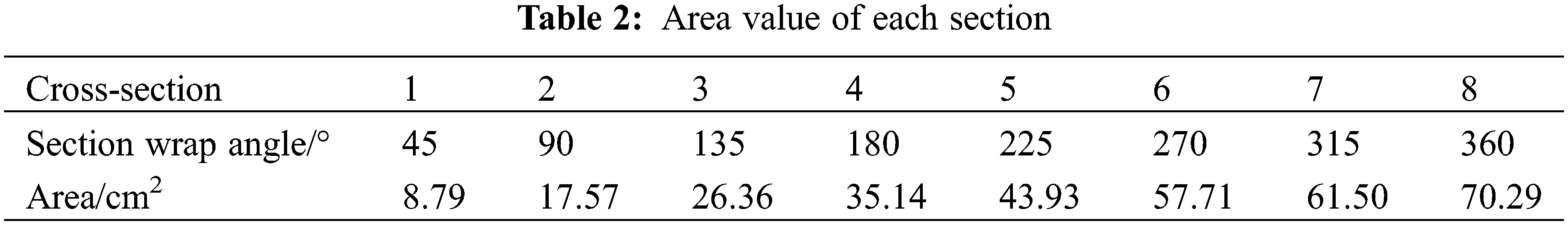
(4)    Area of each cross section

Similar conversions using the velocity factor method

v3=k32gH (22)

In Eq. (22), the v3− Average velocity of the volute section. H− The single-stage head of the pump. k3− The value of the velocity coefficient, k3 , was found to be 0.34 by according to [1].

The calculation gives v3 = 10.65 m/s.

The flow rate through the 8th section and the actual flow rate of the plastic centrifugal pump are approximately equal, so the area of the 8th section can be calculated by the following formula:

F8=Qv3 (23)

The rest of the cross-sectional area is calculated by equalizing the area of each cross-section

Fφ=φ360F8 (24)

The area of each section was obtained as shown in Table 2 below.

2.4 The Main Parameters of the Hydraulic Design of the Inducer

The inducer structure designed in this paper adopts the simpler conical variable pitch form, and its structural form is shown in Figs. 2 and 3.

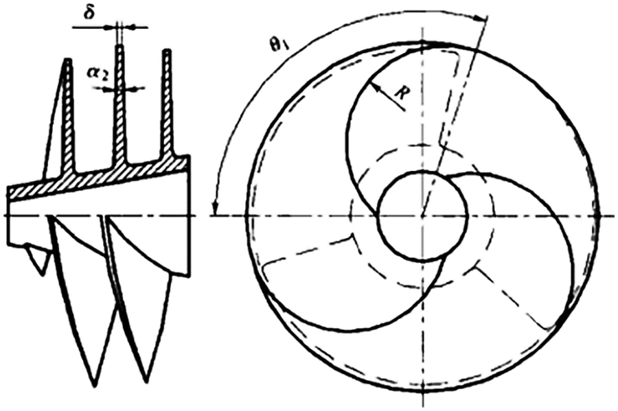
Figure 2: Structure diagram of variable pitch inducer

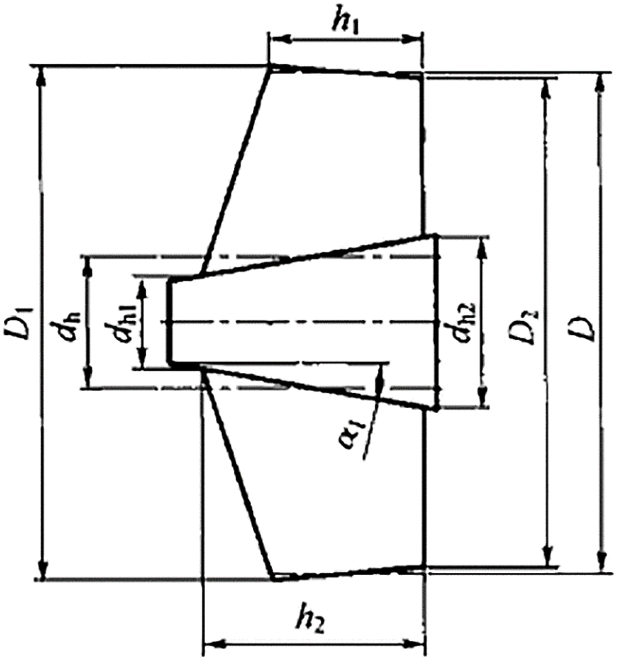
Figure 3: Projection of the axial surface of the inducer

(1)    Number of blades

Theoretically speaking, the number of blades of the inducer to take 1 is the most ideal, in the conditions of the inducer blades on the liquid flow of the smallest crowding effect. But a single blade of the inducer pitch increases, the axial length increases, the hydraulic loss will increase, making it more difficult to manufacture, so the number of blades Zi is generally

Zi=2∼3 (25)

(2)    Inlet flow coefficient and leaf tip diameter

The inlet flow coefficient Φind has an important influence on the shaft power and cavitation performance of the high-speed pump, and the inlet flow coefficient is determined in the case of a fixed flow rate and speed, and the tip diameter of the inducer is also determined. Φind With smaller values, the cavitation performance of the inducer is relatively good. The literature [18] concluded on the basis of experiments that the best cavitation performance of the inducer is obtained when Φind = 0.0645. However, Φind takes a smaller value. The impeller tip diameter has to be increased, which is not conducive to the increase of pump shaft power. Taking into account the cavitation performance and shaft power, the value of Φind can be taken as [19].

Φind=0.06∼0.11 (26)

The inducer tip diameter Dt is taken as

Dt=42∼70mm (27)

(3)    Leaf grid consistency and leaf pitch

The inducer grid consistency is equal to the ratio of the blade spread length and pitch, which has a certain degree of influence on the cavitation performance of the inducer, Chebanowski [20] derived the relationship between the cavitation coefficient of the inducer and the grid consistency through experiments, at the number of blades Zi = 2∼4, if τ≥3 , the axial length of the inducer increases, the energy loss increases, so the range of values of τ should be

τ=2.0∼3.0 (28)

The blade pitch is given by the equation

t=πDtZi (29)

The calculation can be obtained.

(4)    Inlet punch angle αind and blade mounting angle βind

The inlet flow coefficient ϕind is determined, also determine the inlet liquid flow angle of the inducer βi , and the inlet blade installation angle of the inducer βind , then the inlet impulse angle αind and the liquid flow angle βi and, and the guide range S=πDttgβind , so determine the ϕind on the determination of S. Theoretically, αind take a smaller value can make the inducer to achieve higher cavitation performance, but the inducer must produce the pressure head that can make the centrifugal wheel work without cavitation, so αind can not be too small. According to the design practice and experience, it is desirable to

αind=3∘∼5∘≈arctan⁡Φind (30)

βi1=arctan⁡Φind+αind=7∘∼10∘ (31)

For the variable pitch inducer, the inlet liquid flow impulse angle αind can be taken as zero or a smaller value, i.e., the inlet blade installation angle βi is equal to or slightly greater than the inlet liquid flow angle

βi1=arctan⁡Φind+0∘∼2∘ (32)

The exit blade installation angle of the variable pitch inducer βi2 is large to ensure that the exit head generated by the inducer can meet the energy requirements of the centrifugal wheel inlet. Under the design conditions, the centrifugal wheel is generally designed with a positive impulse angle and its blade inlet installation angle βi1=16∘∼22∘ . Therefore, the outlet blade installation angle of the variable pitch inducer βi2 can be taken as

βi2=12∘∼20∘ (33)

The blade processing of variable pitch inducer is more troublesome, and its processing method is different from the impeller blade processing method, so its angle change law cannot use the equal arc arrangement law or logarithmic spiral law.

(5)    Import/export hub ratio

In order to make the inducer have better cavitation performance, the inlet hub ratio Rd1 should be taken as a smaller value, which is generally desirable

Rd1=0.15∼0.28 (34)

The exit hub ratio Rd2 should be taken as the larger value.

Rd2=0.45∼0.65 (35)

(6)    Leading edge wrap angle and leaf tip wrap angle

The inducers have the best cavitation performance less when the leading edge wrap angle is θ1=180∘ [20]. In practice, the cavitation performance of the inducer at θ1=90∘∼150∘ is close to that at θ1=180∘ , and the shorter axial length is favorable for machining. Considering all together, it should be taken

θ1=90∘∼150∘ (36)

The head and axial length of the leaf tip wrap angle of the equal-pitch inducer are calculated by Eqs. (37) and (38), respectively

θ2=360tτsin⁡βi1s (37)

L=θ1+θ2360S (38)

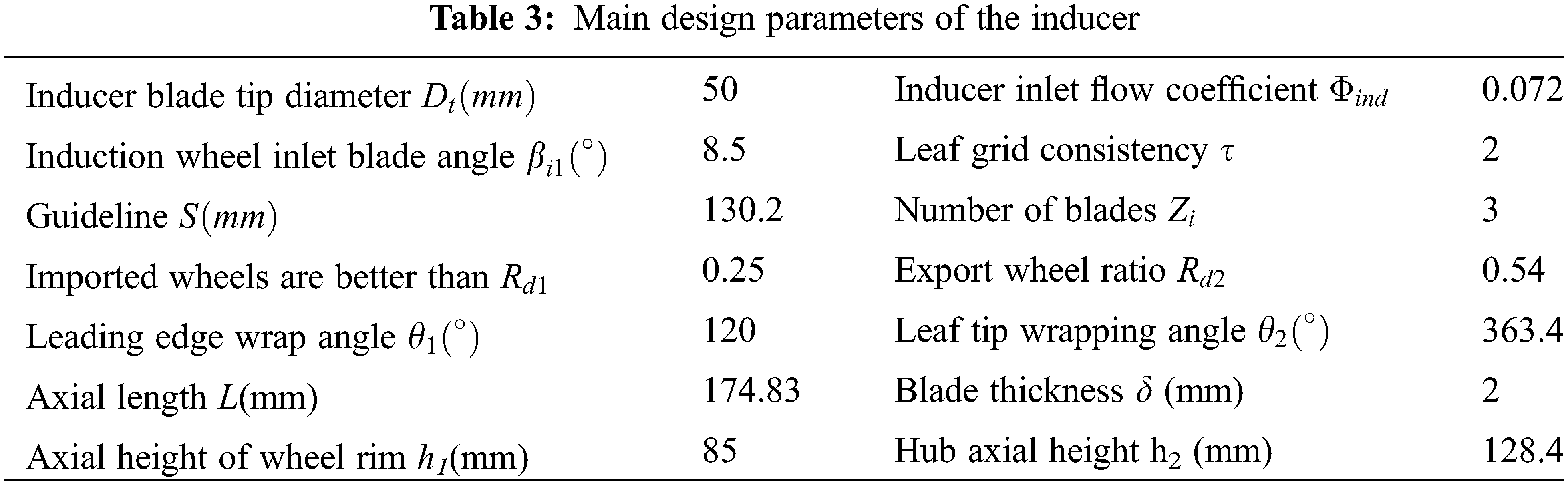
According to the above calculation formula, the specific design parameters of the inducer are as follows in Table 3.

3  Numerical Simulation of Inducer

Computational Fluid Dynamics (CFD) is a systematic analysis of physical phenomena including fluid flow and heat conduction by means of computer numerical calculations and image display, and is applicable to right-angle/columnar/rotary coordinate systems, steady/unsteady flows, transient/slip grids, incompressible/weakly compressible/compressible fluids, buoyant flows, multiphase flows, and non-Newtonian fluids.

The CFD solution process mainly includes the discretization of mathematical equations and solution methods, the establishment of the computational grid, the setting of boundary conditions and the post-processing of the computational data. Among them, the establishment of the control equations, the grid division and the setting of the boundary conditions are the prerequisite and key to the numerical calculation.

3.1 Flow Control Equation

The fluid dynamics control equations include the continuity equation, the momentum equation and the energy equation, and the flow inside the impeller machinery is subject to these three equations [21], and the energy conservation equation is not considered due to the relatively small amount of heat exchange involved in the calculations of this paper.

(1)    Conservation of mass equation

The mass conservation equation, also known as the continuity equation, is a change in the total amount of some conserved quantity in any region, equal to the amount entering or leaving from the boundary; the conserved quantity cannot increase or decrease, but can only be transferred from one location to another.

∂ρ∂t+∂(ρu)∂x+∂(ρv)∂y+∂(ρw)∂z=0 (39)

where, ρ is the fluid medium density, t is the time quantity, and u, v, and w are the components of the velocity vector in the x, y, and z directions, respectively.

(2)    Conservation of momentum equation

The conservation of momentum equation is a fundamental law that must be satisfied by any flow system, and is actually Newton’s second law, which is defined as: the rate of change of momentum in any control micro-element produced by a change in time is equal to the sum of external forces acting on the micro-element.

∂(ρu)∂t+u∂u∂x+v∂u∂y+w∂w∂z=−∂p∂x+∂τxx∂x+∂τyx∂y+∂τzx∂z+Fx (40)

∂(ρv)∂t+u∂v∂x+v∂v∂y+w∂v∂z=−∂p∂x+∂τxy∂x+∂τyy∂y+∂τzy∂z+Fy (41)

∂(ρw)∂t+u∂w∂x+v∂w∂y+w∂w∂z=−∂p∂x+∂τxz∂x+∂τyz∂y+∂τzz∂z+Fz (42)

where τxx , τyy and τzz are the components of the viscous force τ in the x, y and z directions; Fx, Fy and Fz are the volume forces acting on the micro-element in the x, y and z directions. In this paper, the values of Fx, Fy and Fz are 0; p is the pressure on the micro-element.

If the working medium is a Newton fluid, then there is

τxx=2μ∂u∂x+λdiv(u);τxy=τyx=μ(∂u∂y+∂v∂x) (43)

τyy=2μ∂v∂y+λdiv(u);τxz=τzx=μ(∂u∂z+∂w∂x) (44)

τzz=2μ∂w∂z+λdiv(u);τyz=τzy=μ(∂v∂z+∂w∂y) (45)

where, μ is the dynamic viscosity, λ is the second viscosity, according to experience can generally take λ = 2/3, the above formula can be substituted to get.

∂(ρu)∂t+div(ρuu)=div((μ+μT)gradu)−∂p∂x+Su (46)

∂(ρv)∂t+div(ρvu)=div((μ+μT)gradv)−∂p∂y+Sv (47)

∂(ρw)∂t+div(ρwu)=div((μ+μT)gradu)−∂p∂z+Sw (48)

where grad() = ∂ ()/ ∂ x + ∂ ()/ ∂ y + ∂ ()/ ∂ z and the symbols Su, Sv and Sw are the generalized source terms of the momentum conservation equation, Su = Fx + Sx, Sv = Fy + Sy, Sw = Fz + Sz, and Sx = Sy = Sz = 0 for incompressible flow.

3.2 Turbulence Model

The shear stress transport k-ω model (SST k-ω model for short), proposed by Menter, combines the respective advantages of the standard k-model and the standard k-ε model, with the addition of the transverse dissipative derivative term and cross-diffusion in the ω equation in the SST k-ω model compared to the two base models. This feature makes it more applicable to a wider range of applications and has higher accuracy and confidence. The model equations are.

∂(ρk)∂(t)+∂(ρujk)∂xi=∂∂xi[(μ+μtσk3)∂k∂xi]+pk−β′ρkω (49)

∂(ρω)∂(t)+∂(ρuiω)∂xi=∂∂xj[(μ+μtσk3)∂ω∂xj]+a3ωkpk−β3ρω2+(1−F1)2ρσω21ω∂k∂xj∂ω∂xj (50)

where pk is the turbulent kinetic energy production rate, whose expression is

pk=μt2Sij∂ui∂xj (51)

Sij=12(∂ui∂xj+∂uj∂xi) (52)

Turbulent viscosity coefficient

μt=ρkω1max[1α∗,SF2a1ω] (53)

where

S=2SijSij (54)

Sij is the spin rate.

F2=tanh⁡(Φ22) (55)

Φ2=max[2k0.09ωy,500μρy2ω] (56)

where, y is the distance to the other face.

The SST k-ω model has been substantially optimized on the standard k-ω model. In order to make the final calculation results more accurate, the model further addresses the shortcomings of the large error near the wall in the calculation.

3.3 Grid Division and Irrelevancy Analysis

To ensure the accuracy of the numerical calculation and to ensure that the near-wall region can have a sufficient number of nodes for capturing the flow within the boundary layer, y+ is usually used. y+ denotes the distance of the nearest grid point to the wall surface and is a dimensionless parameter defined by

y+=Δyρμτwρ (57)

where, Δy is the distance from the node to the wall; τw is the wall shear stress: μ is the dynamic viscosity of the fluid.

The y+ is the basis for choosing the turbulence model, and the turbulence model is chosen differently for different y+ magnitudes. In the numerical simulation of this paper, the calculated y+ value is close to 30, and the turbulence model is chosen as the SST k-ω model, which satisfies its quality requirements [22].

In this paper, ANSYS ICEM CFD software was selected to mesh the model. The mesh delineation is shown as follows (Figs. 4–7).

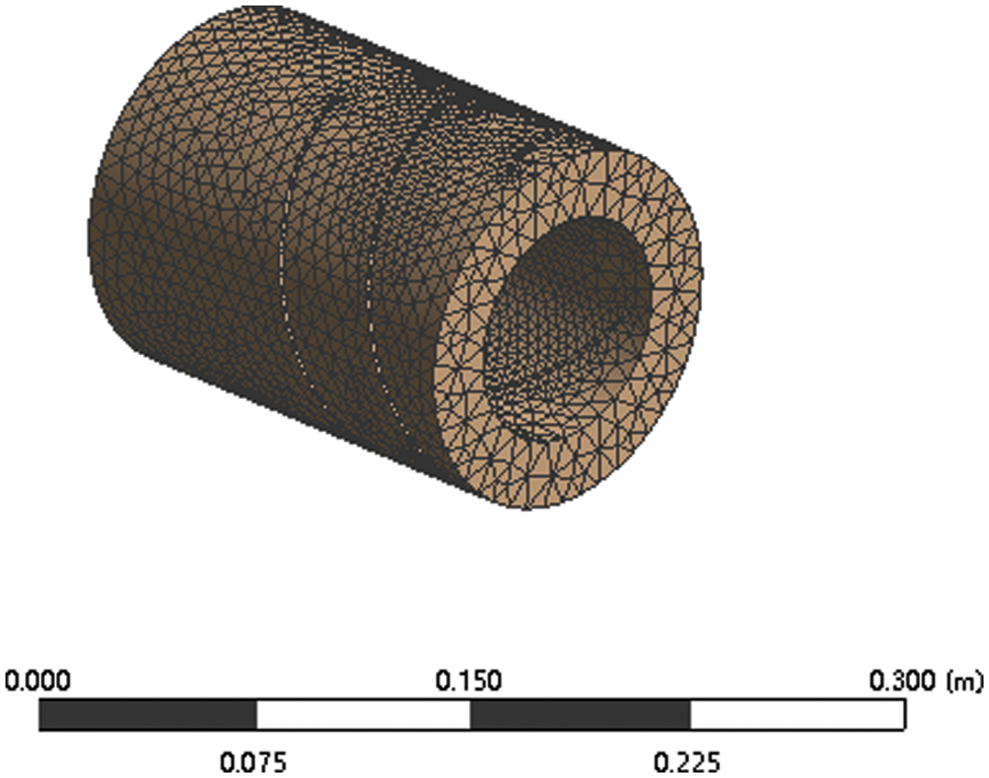
Figure 4: Inducer

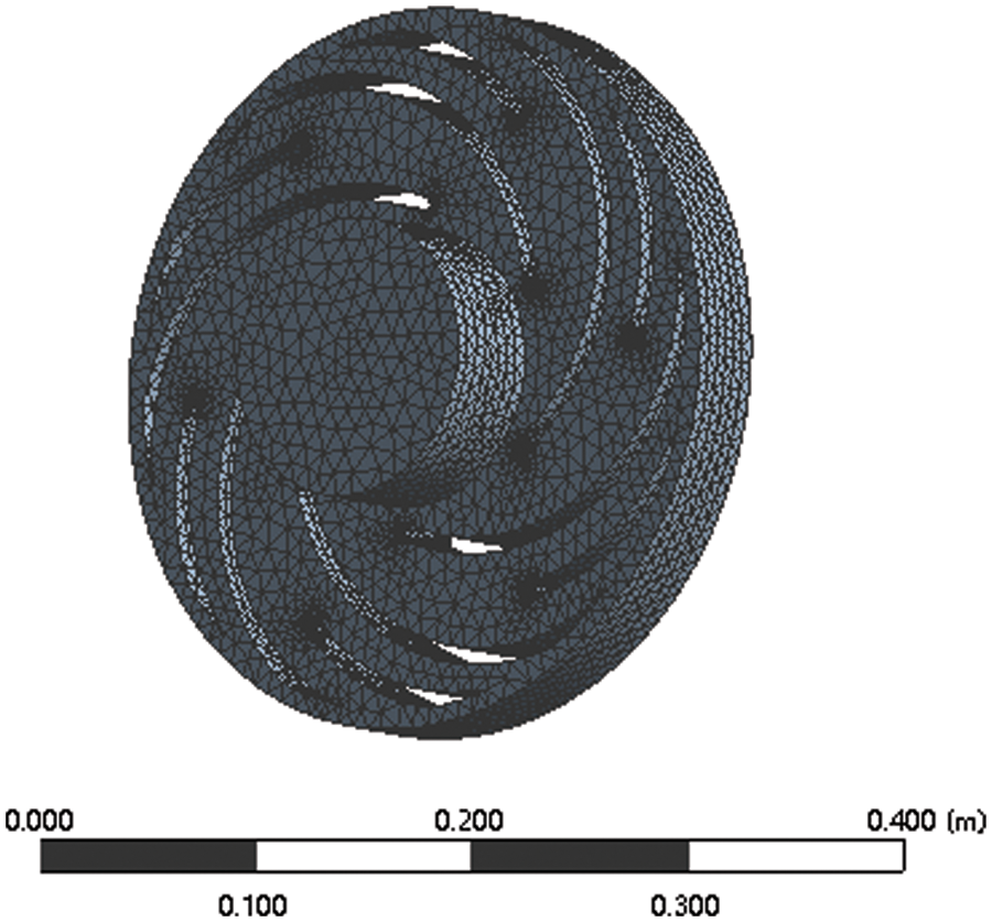
Figure 5: Main impeller

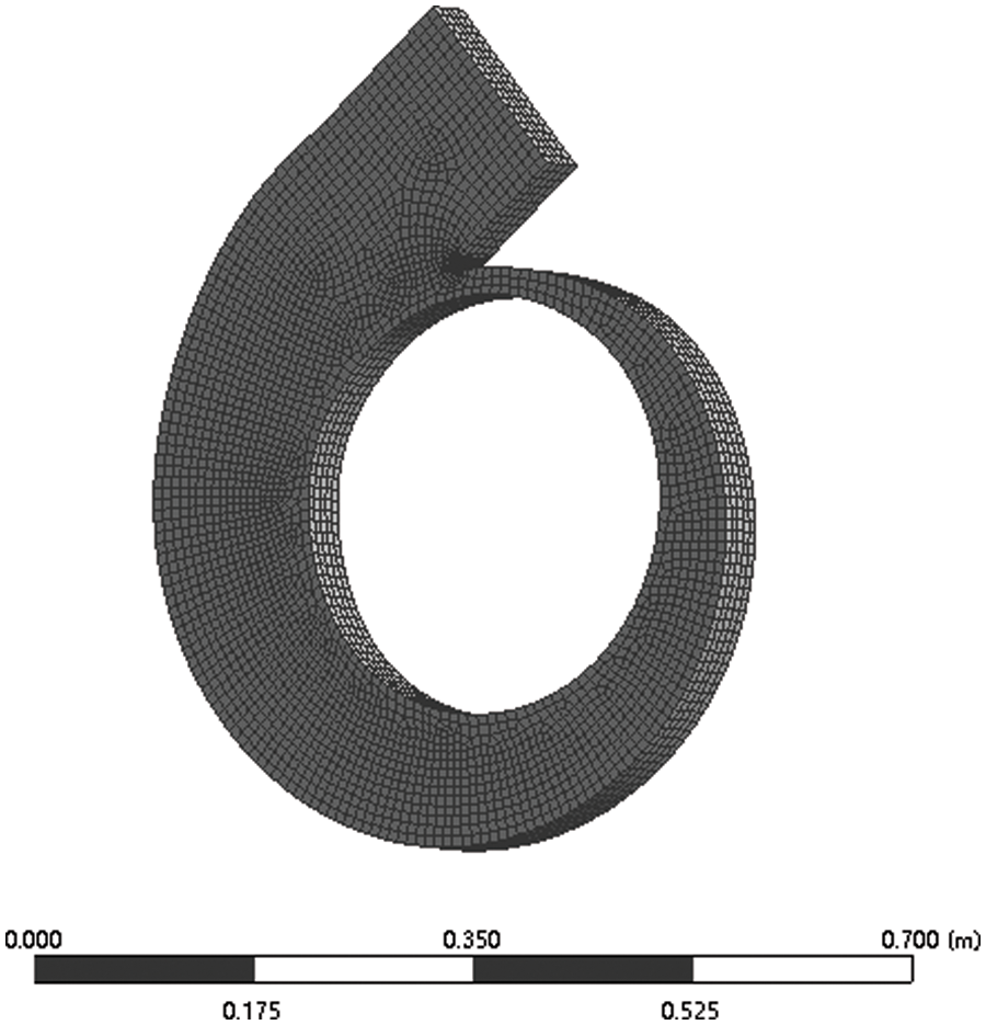
Figure 6: Volute

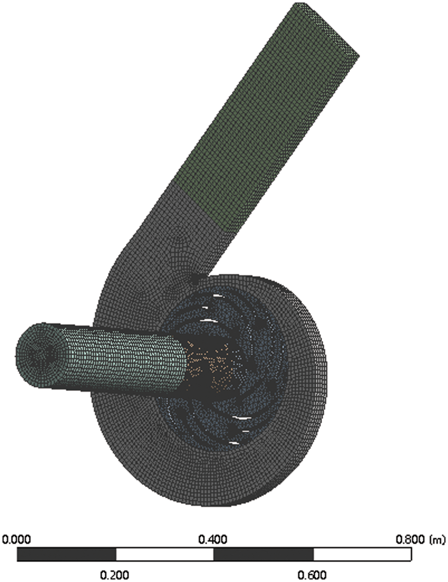
Figure 7: Whole flow field

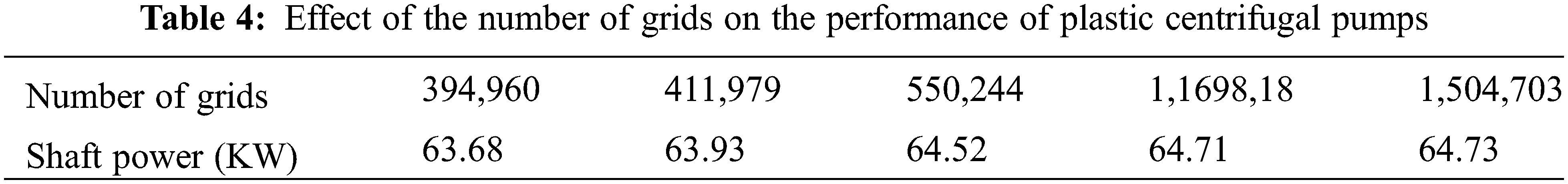
The number of grids will limit the speed and accuracy of the numerical simulation. The smaller the number of grids and the coarser the mesh, the worse the simulation accuracy; the larger the number of grids and the finer the mesh, the longer the simulation time. In order to improve the simulation speed and study the shaft power without affecting the simulation accuracy, it is necessary to verify the grid irrelevance. The centrifugal pump with the same working condition and structure is selected, and the number of grids is changed to simulate the flow field of the whole machine, and the optimal number of grids is derived. The grid irrelevance validation is shown in the following table.

From the data in Table 4, it can be seen that the shaft power of the plastic centrifugal pump keeps a stable trend when the number of grids is above 1,169,818, indicating that when the number of grids reaches 1,169,818, its influence on the simulation results is small and negligible. In order to ensure the simulation speed and save computer resources, the mesh number is controlled to be about 1,169,818 million when the centrifugal pump simulation is carried out.

After the grid irrelevance verification, the number of grid nodes, the number of grids and the quality of grids are determined. The number of nodes in this simulation is 287,970, and there will be about 0.35% floating in different structural models; the number of grids is 397,207, and there is about 0.67%∼1% quantity difference in different models; 75% of the grid quality is 0.96, 22% of the grid quality is 0.63, and 3% of the grid quality is 0.27, and the grid quality is good.

3.4 Boundary Conditions

Inlet boundary conditions: The inlet conditions of the flow are generally set as velocity inlet (for non-pressurizable flow), mass inlet (for pressurizable flow) or pressure inlet (for pressurizable and non-pressurizable flow). In this paper, we choose the pressure inlet boundary condition, and the size of the pressure value is chosen as 1 atm.

Outlet boundary condition: In this paper, the mass flow outlet boundary condition is selected to control the flow rate of the pump. According to the performance parameters of the plastic centrifugal pump, the size of mass flow rate is selected as 69.45 kg/s.

Object surface boundary conditions: The object surface includes the suction surface and pressure surface of the inducer and impeller blade, the wall surface of the axial gap, the front and rear cover of the impeller, the wall surface of the volute and the wall surface of the extension section, etc. Among them, the object surfaces related to the inducer and impeller do rotational motion with the inducer and impeller relative to the absolute coordinate system, and the rest of the object surfaces are relatively stationary. Because the turbulent flow evolves into laminar flow in the near-wall area, it is necessary to use the wall function method for the near-wall area to do the corresponding treatment. Generally, no-slip boundary conditions are used in the solution, and the relative velocity on the wall surface W = 0.

The boundary conditions in CFD calculations also include symmetric boundary conditions and periodic boundary conditions, etc. In this paper, the numerical calculation domain is the flow field of the whole centrifugal pump, and there is no periodicity problem or symmetry problem, so it is not considered.

With the above settings, the structure tree model in Fig. 8 and the fluid domain model in Fig. 9 can be obtained.

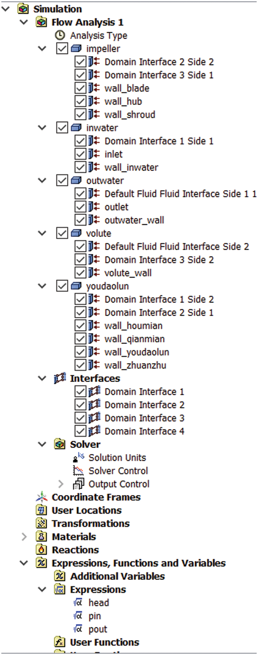
Figure 8: CFX structural tree model

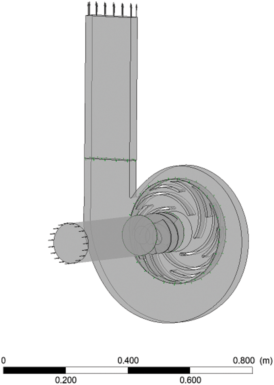
Figure 9: CFX fluid domain model

3.5 Discrete Format

In this paper, the finite volume method is chosen to construct the discrete equations, and in this process the construction of the discrete format needs to be involved. The discrete format is the way in which the physical quantities at the interface of the control body and the nodes of their corresponding derivatives are interpolated. The commonly used discrete formats and their specific formats are described in the literature [23].

In this paper, considering the centrifugal pump flow field as a complex three-dimensional distorted fluid region, in order to ensure the unity of solution compatibility, convergence and stability in the numerical solution process. Therefore, the absolute stable windward format is chosen to solve the equations. First, the first-order windward format is used to solve the corresponding flow domain, and after reaching the convergence condition, the second-order windward format is used to continue the solution until convergence on the basis of the original solution results in order to improve the accuracy of the calculation.

3.6 Flow Field Analysis

After the CFX-Pre is defined, the solution is performed using the stability solver. In this paper, a time step of 3° of impeller rotation is chosen for the non-constant numerical calculation. According to the speed of centrifugal pump 2700 r/min, the time step of each step is calculated as 0.006 s (i.e., impeller rotation 3°), and the total calculation time is 11.52 s (i.e., impeller rotation 16 revolutions), the maximum number of iteration steps for the non-constant calculation is 1000, and the convergence criterion is the average value RMS with the value 1.E-5, and the SIMPLEC algorithm is used to calculate, and after the curve After convergence, pressure nephograms of the plastic centrifugal pump impeller and inducer impeller are obtained as follows Figs. 10–12.

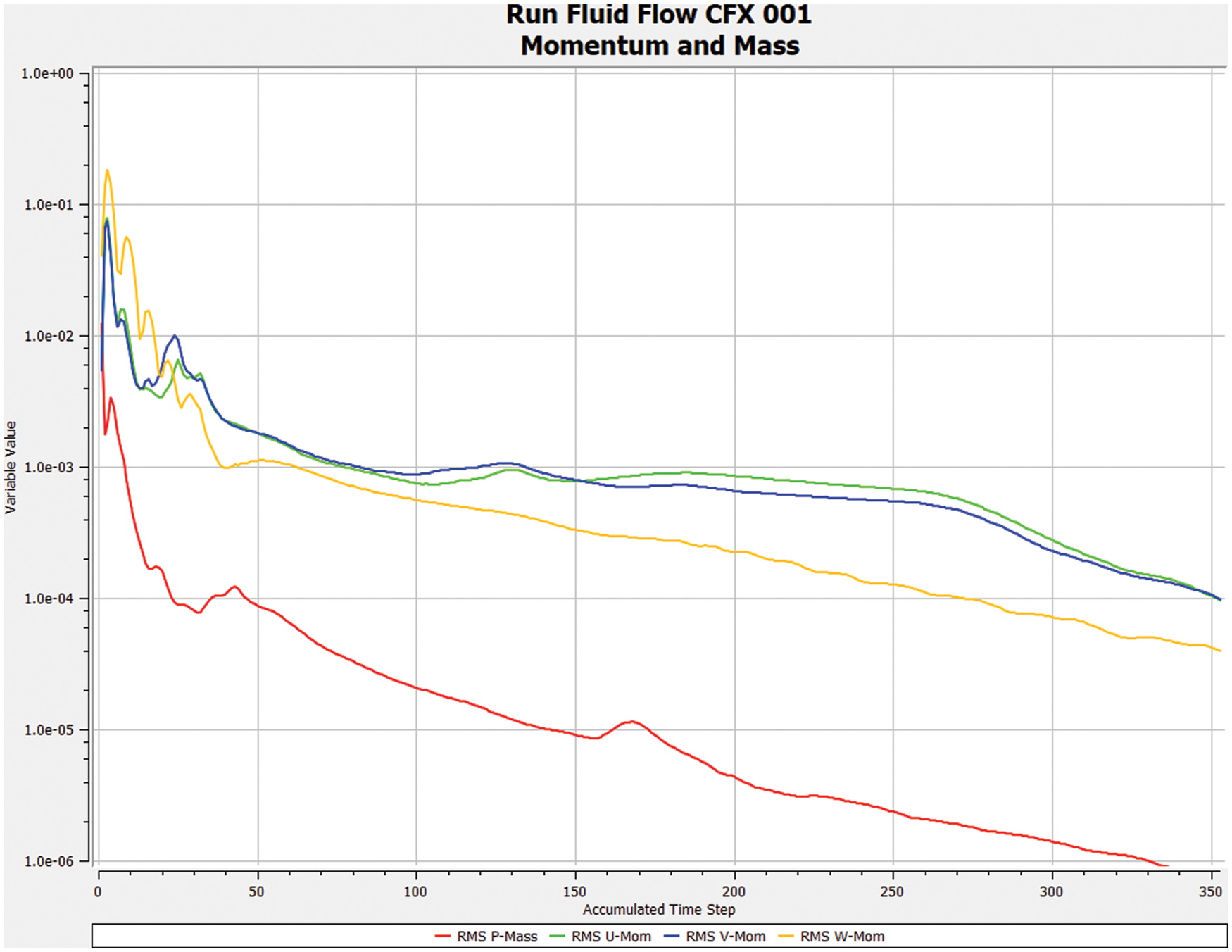
Figure 10: Residual curve graph

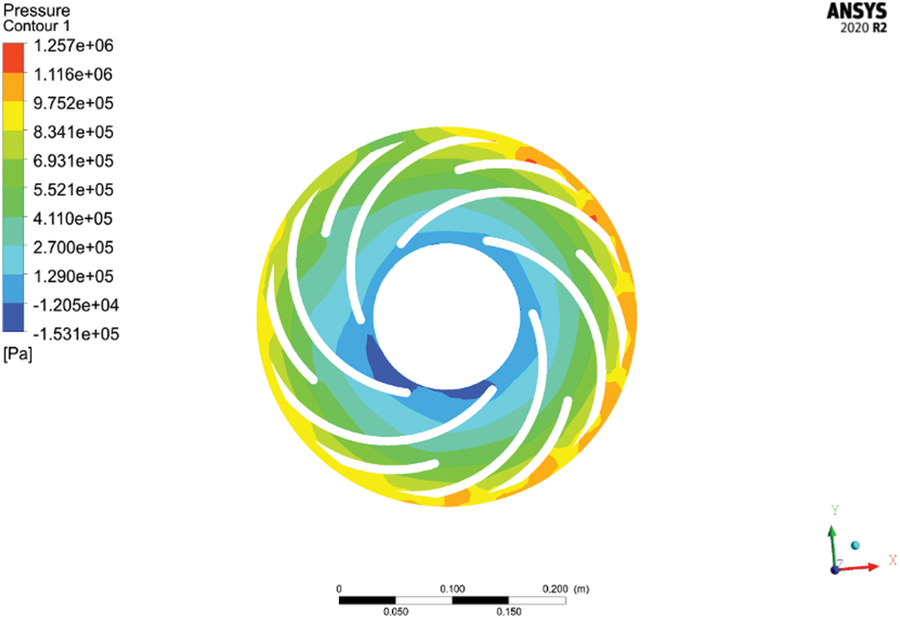
Figure 11: Impeller pressure nephogram diagram

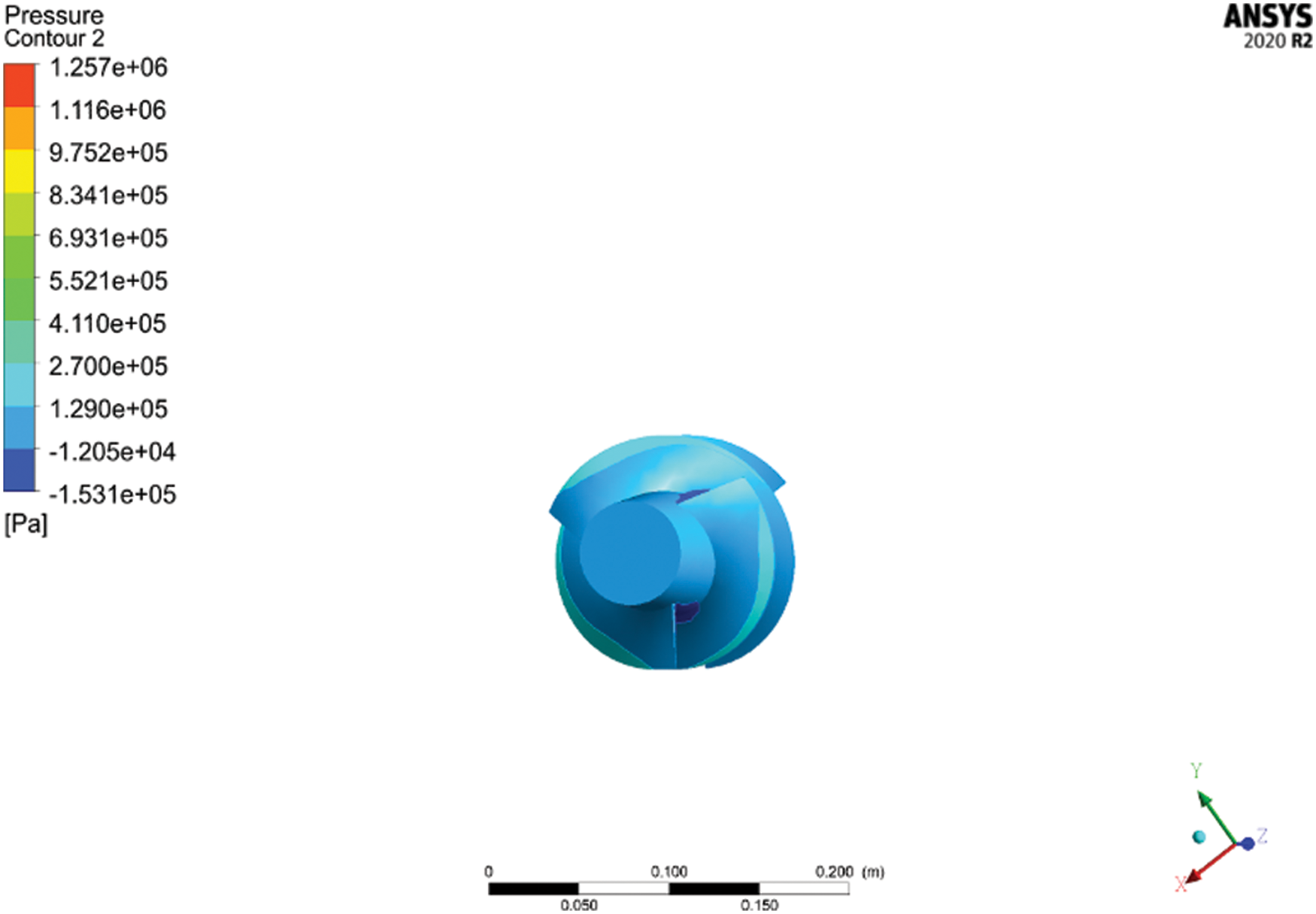
Figure 12: Inducer pressure nephogram

Fig. 11 shows the pressure distribution diagram of the impeller of the plastic centrifugal pump. Analysis of Fig. 11 shows that the pressure value from the impeller inlet to the impeller outlet is gradually increasing, indicating that the impeller rotates during the process of doing work on water, which makes the water pressure gradually increase from the impeller inlet to the impeller outlet, and the water then reacts to the impeller, so that the impeller pressure appears to increase circumferentially.

Fig. 12 shows the pressure distribution of the impeller of the inducer. Analysis of Fig. 12 can be obtained, from the figure can be seen, the inducer impeller blade surface static pressure from the inlet to the outlet showing an increasing trend, blade pressure surface pressure is higher than the blade suction surface pressure, the lowest pressure area are in the blade suction surface inlet position.

4  Orthogonal Experimental Design of Structural Parameters of Plastic Centrifugal Pump

4.1 Orthogonal Experimental Design

The orthogonal test is a common experimental design scheme for solving multi-factor tests through the appropriate design of experimental protocols with orthogonal tables specified in mathematical statistics. The basic steps are shown below:

(1)    Clear test objectives, determine the test indicators

In the orthogonal test design of the selected parameters, the test indexes should be clarified and the quality evaluation indexes should be determined.

(2)    Selection of test factors and determination of their test levels

In the orthogonal test, the factors are shown in English A, B, etc., instead. When determining the test factors, the priority is given to the factors that have a greater influence on the test evaluation index. In order to obtain higher experimental efficiency, the number of factor level values is usually chosen from 2 to 4, and the interval of level values should be reasonable.

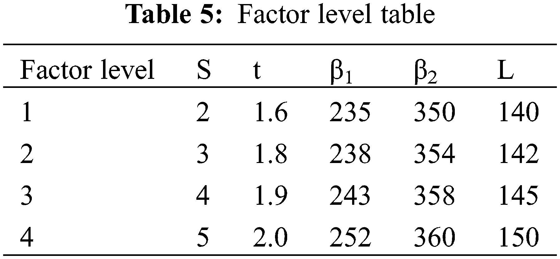
4.2 Determination of the Factor Level Values

In this test, there are many factors affecting the head and shaft power, according to the relevant theory and requirements, selected blade thickness, lobe degree, blade flange angle, blade hub angle and hub length as the five factors of the orthogonal test, The selected factors and their level values are shown in Table 5, for the convenience of describing the results of the extreme difference analysis, they are denoted by A, B, C, D, E blade thickness S, cascade solidity t, blade rim angle β1, blade hub angle β2, hub length L, respectively.

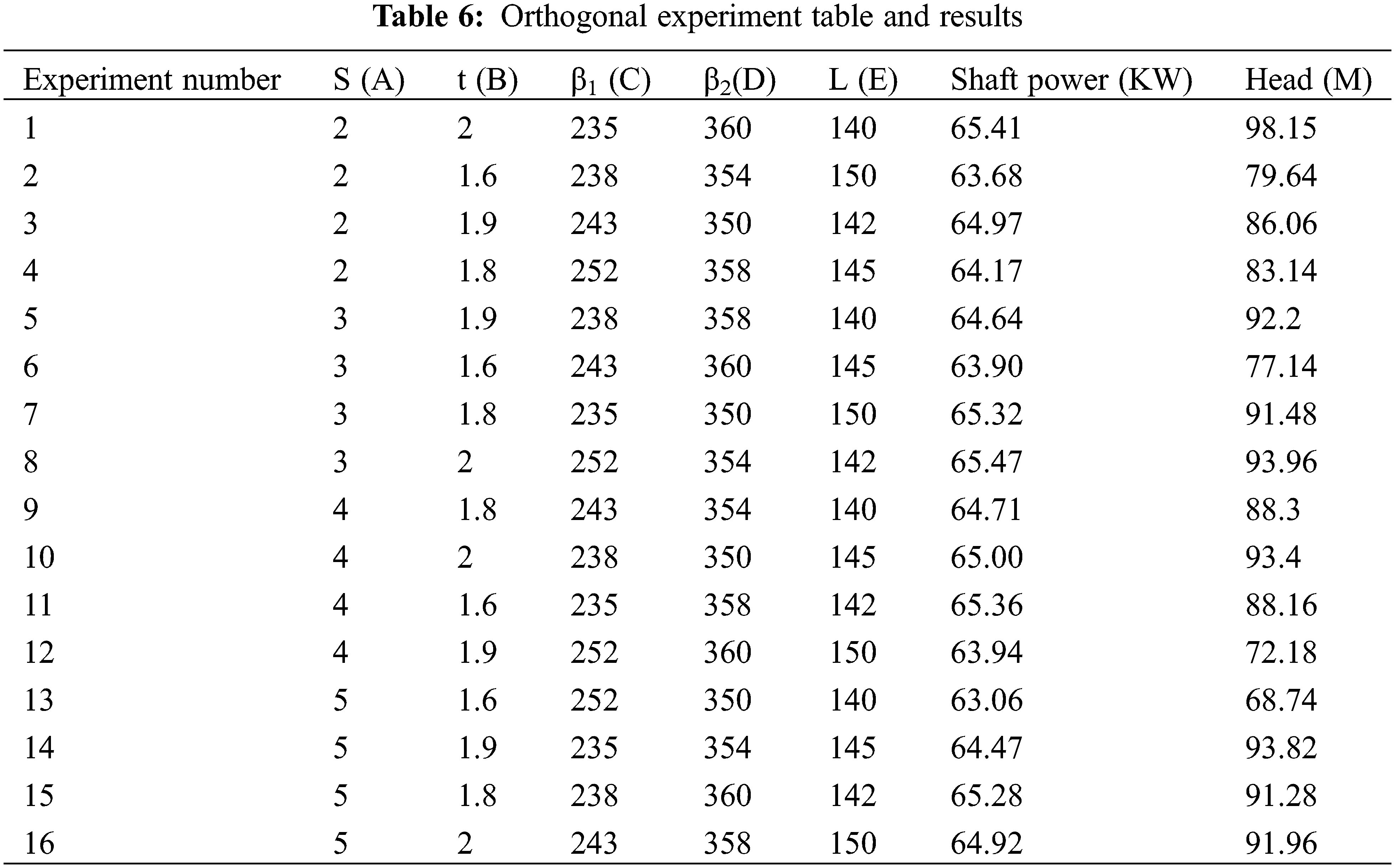
4.2.1 Orthogonal Experimental Results and Range Analysis

For the five-factor four-level orthogonal experiments can be selected from the orthogonal table L16 (165), and through the CFX simulation software for the orthogonal test permutations of 16 groups of parameters one by one numerical simulation, and the results were calculated to obtain the specific orthogonal experimental results are shown in Table 6.

4.2.2 Data Processing of the Experimental Results

According to the experimental results in Table 6, the R-value of each parameter is calculated, and the magnitude of the influence of each factor (parameter) on the index (shaft power, head) can be clearly seen in Tables 7 and 8.

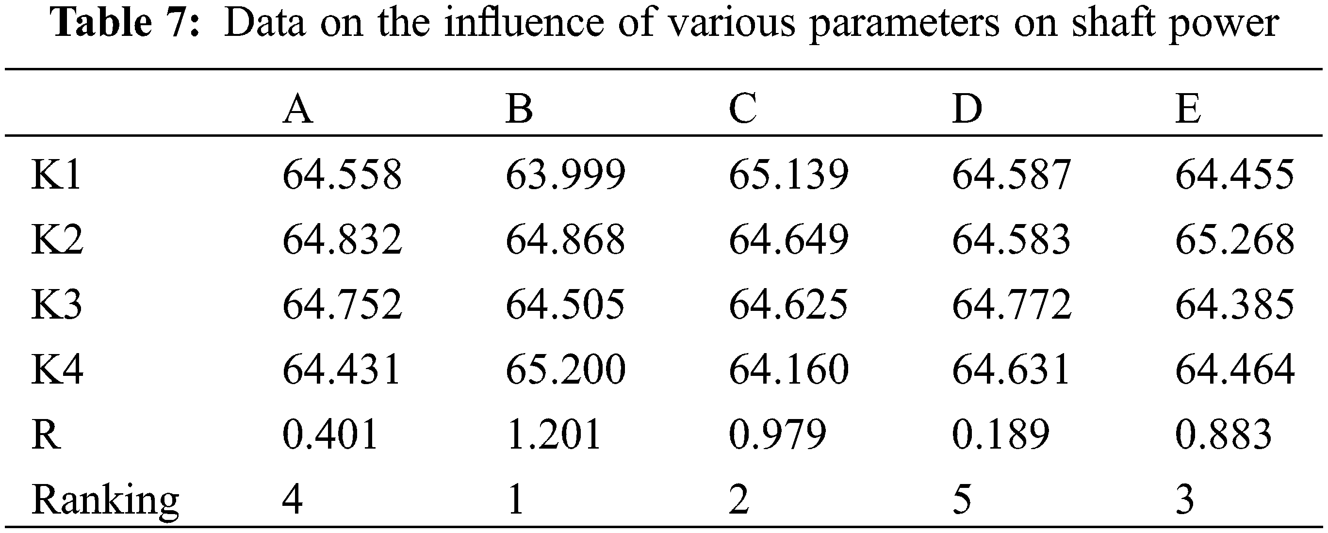
(1)    Table 7 shows the results obtained with the shaft power as the evaluation index:

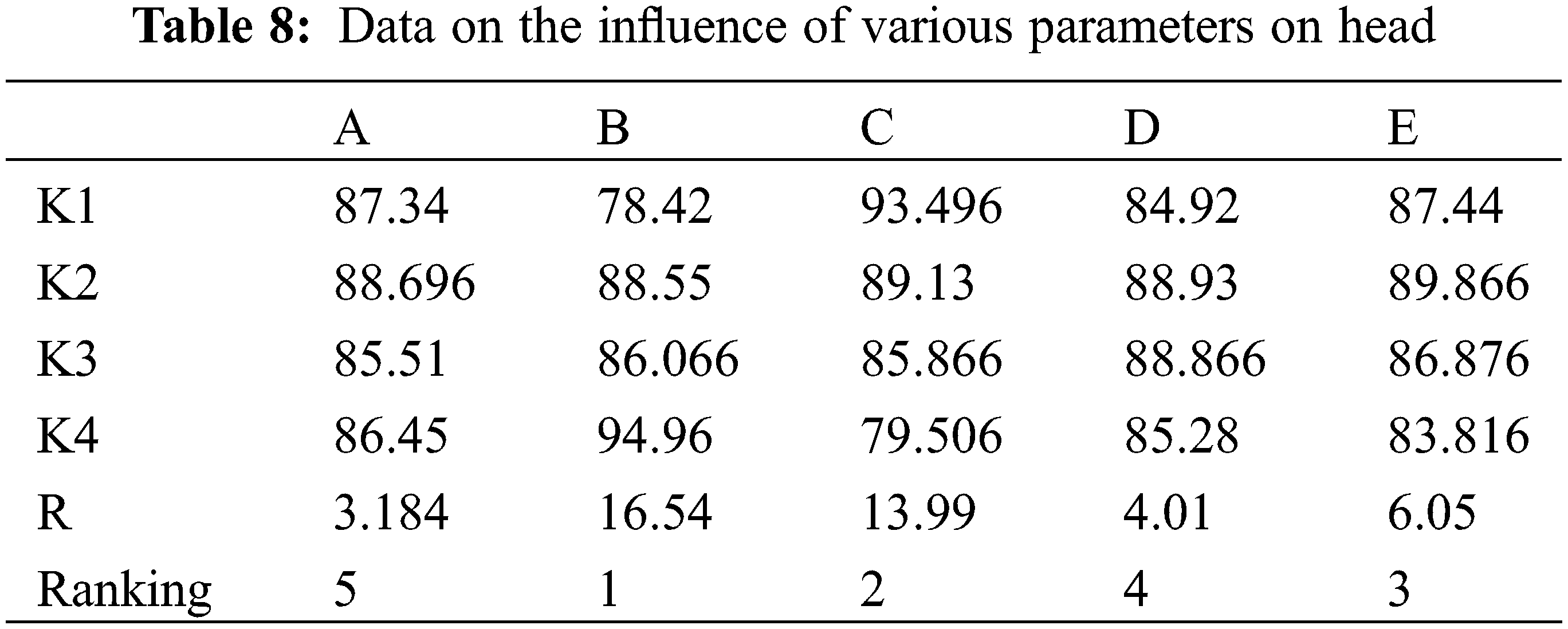
(2)    Table 8 shows the results obtained with the head as the evaluation index:

4.2.3 Analysis of the Experimental Results

1.    For the shaft power

In Table 7, Kl, K2, K3 and K4 denote the sum of the axial power values of each factor at the 1st, 2nd, 3rd and 4th levels, respectively, and the size of the extreme difference R reflects the degree of influence of each factor on the axial power. According to the evaluation index, the best combination is obtained as A4 B1 C4 D4 E1, that is, when the inducer blade thickness is 5 mm, the cascade solidity is 1.6, the blade rim angle is 252°, the blade hub angle is 350°, and the hub length is 140 mm, the minimum shaft power can be obtained.

The results of the orthogonal experiments were processed using the extreme difference analysis method, and the trend of the influence of each influencing factor on a single evaluation index can be obtained. The order of the influence of each parameter on the shaft power is: Cascade solidity > blade rim angle > hub length > blade thickness > blade hub angle.

2.    For the head

In Table 8, Kl, K2, K3 and K4 denote the sum of the head values of each factor at the 1st, 2nd, 3rd and 4th levels, respectively, and the size of the extreme difference R reflects the degree of influence of each factor on the shaft power. According to the evaluation index, the best combination of is obtained as A1 B4 C1 D4 E1, that is, When the blade thickness, cascade solidity, rim angle, hub angle, and hub length were 2 mm, 2, 235°, 360°, and 140 mm, respectively, the maximum head can be obtained.

The results of the orthogonal experiments were processed using the extreme difference analysis method, and the trend of the influence of each influencing factor on a single evaluation index can be obtained. The order of the influence of each parameter on the shaft power is: Cascade solidity > blade rim angle > hub length > blade hub angle > blade thickness.

5  Parameter Optimization of Inducer Structure Based on Least Squares and Fish Swarm Algorithm

5.1 The Least-Squares Method

It is a method to find out the curve by using mathematical formulae or computer-aided methods when the data of X and Y are known. In essence, it is a data processing method that approximates the discrete point data according to the analytical expressions, and approximates the relationship between the discrete point data by continuous smooth curves, and finds the relationship between the variables from these discrete point data, thus reflecting the change pattern of the discrete point data [24].

5.2 Least Squares Curve Fitting

(1)    Set weights

In this paper, five factors are integrated into one by using the way of setting weights, and by referring to relevant information and considering the actual situation in the process of optimizing the structural parameters of the inducer, the weights of each factor are set as follows:

ω=(ω1,ω2,ω3,ω4,ω5)=(0.4,0.3,0.1,0.1,0.1) (58)

(2)    Numerical calculation

Using the weight values to weight the 16 sets of structural parameter combinations, the obtained is the X among the least squares method, whose values are 74.9, 75.48, 74.87, 76.84, 75.37, 76.48, 75.24, 76.6, 75.84, 75.5, 75.58, 78.37, 76.68, 75.97, 76.54, and 77.7. The evaluation indexes in this paper are shaft power and shaft power, so the Y values in the least squares fit are the values of head and shaft power for the 16 groups in the orthogonal test table, which can be obtained by checking Table 5.

(3)    Curve fitting

In order to make the curve fitting more accurate, the weighted obtained data were imported into Matlab and the discrete points were connected, as in Fig. 13.

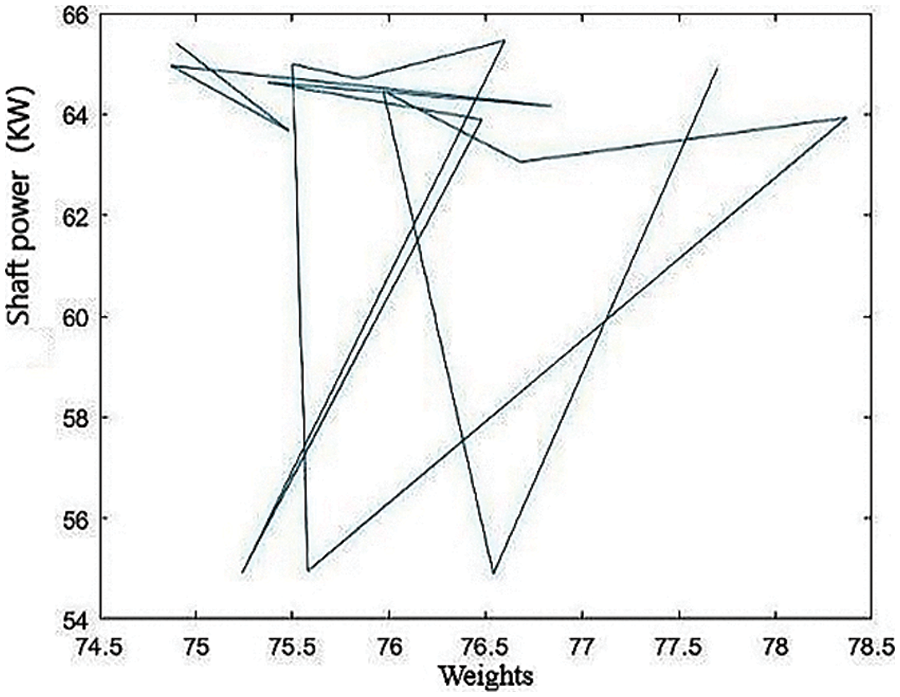
Figure 13: Data import

Fig. 13 shows the data distribution obtained after automatic import using Matlab software. Next, the software was used to simulate the curve for this set of discrete data, and through several attempts and optimization, the final fitted curve is shown in Fig. 14.

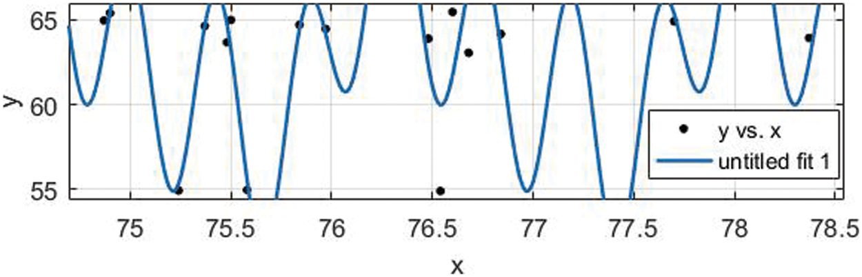
Figure 14: Fitting curve

As shown in Fig. 14, the imported 16 sets of data are basically distributed on the fitted curve, and some points deviate from the fitted curve, because curve fitting itself is a process of infinite approximation, and it is impossible to guarantee that all the discrete points are on the fitted curve, but it is an important evaluation index to ensure that as many as possible are on the curve, so the fitted curve meets the requirements from the overall point of view. The analytic equation of the curve after fitting by the software is a 4th order Fourier polynomial. And Fig. 15 is a schematic diagram of fish school optimization, which mainly shows the activity state of fish school.

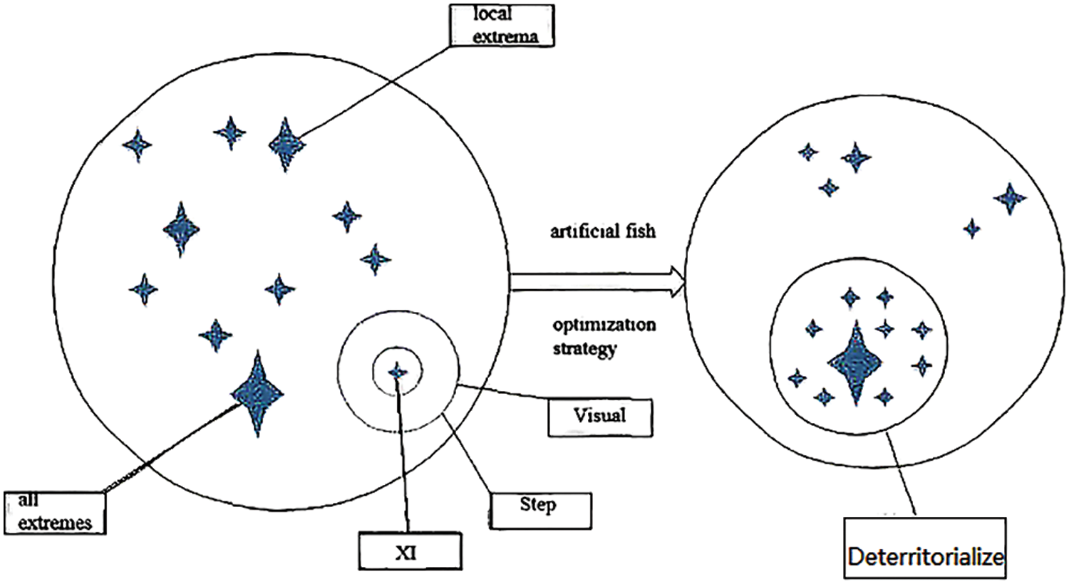
Figure 15: Schematic diagram of fish school optimization

5.3 Optimization of Structural Parameters Based on Fish Swarm Algorithm

5.3.1 Introduction to Fish Swarm Algorithm

The artificial fish is constructed with the characteristics of fish, imitating the behavior of fish swarms, each fish corresponds to an optimization solution, the virtual water corresponds to the solution space of the optimization problem, and the food concentration corresponds to the objective function value, and the optimization search is achieved by the fish swimming in the virtual water [25]. Fig. 16 represents a flow chart of the algorithm used in this paper, and Fig. 17 shows a schematic diagram of each parameter.

(1)    Foraging behavior: Let the current state of the artificial fish be Xa ; choose a random state within its field of view Xb , for

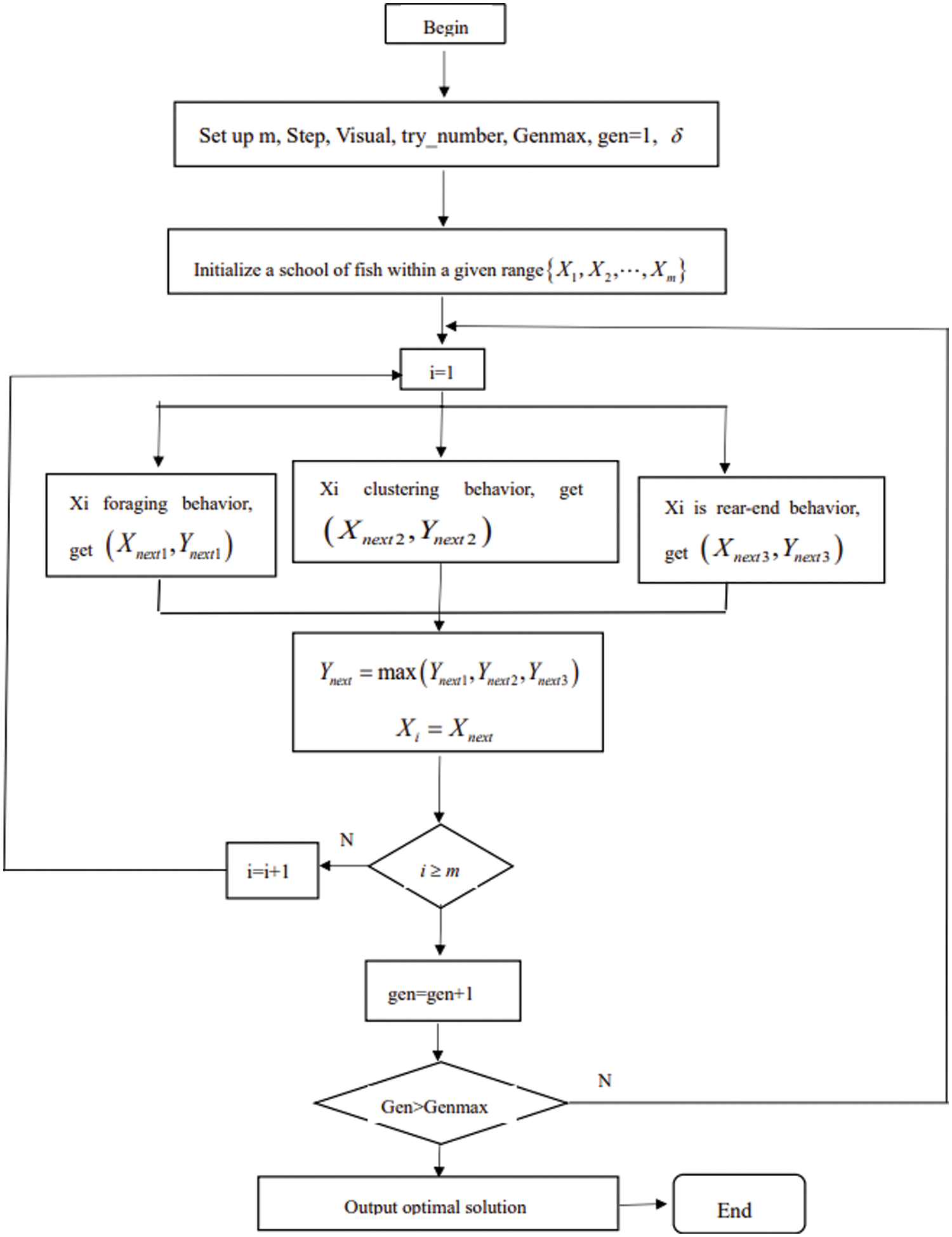
Figure 16: Algorithm flow chart

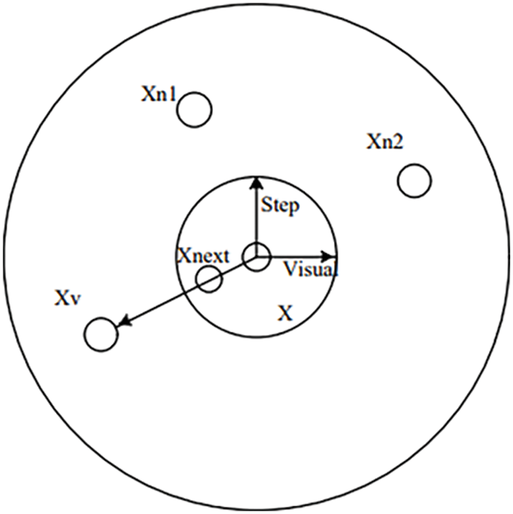
Figure 17: Schematic diagram of each parameter

Xb=Xa+Visual⋅Rand() (59)

If the food concentration Ya > Yb, then a step forward in that direction is

Xat+1=Xat+Xb−Xat‖Xb−Xat‖Step⋅Rand() (60)

(2)    Clustering behavior: Let the current state of the artificial fish be Xa , detect the number of partners in its neighbourhood nf , if nf/N<δ , indicating that there is more food and less crowded in the center of the partners, and Ya>Yc , then move one step forward to the central position Xc , for

Xat+1=Xat+Xc−Xat‖Xc−Xat‖Step⋅Rand() (61)

Otherwise, perform other acts.

(3)    Tail-chasing behavior: Let the current state of the artificial fish be Xi , detect its neighbour Xmax with the best state in its neighborhood, and if Ya>Ymax and the number of partners in the neighborhood of Xmaxnf satisfies nf/N<δ , indicating that there is more food and less crowded in the vicinity of Xmax , then move forward in the direction of Xmax , as

Xat+1=Xat+Xmax−Xat‖Xmax−Xat‖Step⋅Rand() (62)

Otherwise perform foraging behavior.

(4)    Random behavior: in essence, a default default behavior for foraging behavior

Xat+1=Xat+Visual⋅Rand() (63)

(5)    Bulletin board: It is mainly used to record the status of the optimal artificial fish individuals during the optimization process [26–30].

5.3.2 Optimization Process of Fish Swarm Algorithm

(1)    Mathematical model input and initialization settings

According to the specific situation of this paper, the number of artificial fish is set to 50; from the practical consideration, the maximum number of iterations is set to 50 and the maximum number of tries is 100; the perceptual distance is set to 1; the congestion factor is set to 0.618; finally, the merit-seeking step is set to 0.1.

(2)    Analytical calculations

After the initial setup, the algorithm will be run and the computer will perform internal calculations based on the set parameters to solve for the adaptation values of individual fish, based on which the best artificial fish state will be selected by comparison and assigned to the bulletin board.

5.3.3 Optimization Results of the Fish Swarm Algorithm for the Structural Parameters of the Inducer

In the initialization setup of 5.3.2, the parameters required for the execution of the algorithm were input into the algorithm program, and then the fish swarm algorithm program was imported into Matlab for the merit search analysis. After several debugging and testing, the results are shown in Figs. 18 and 19.

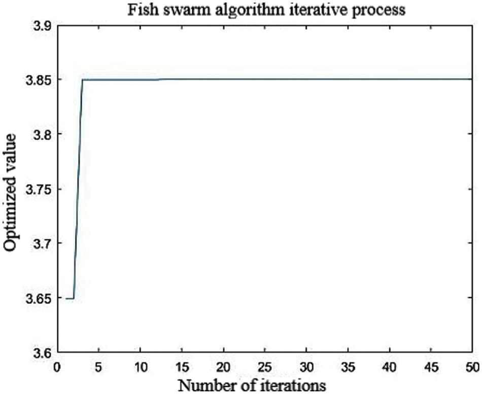
Figure 18: Number of iterations

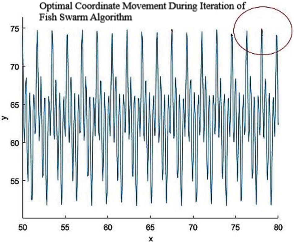
Figure 19: Location of optimal solution

By analyzing the results in Fig. 19, it can be concluded that the optimal solution X obtained by the artificial fish swarm algorithm optimization is 77.8762, which is approximately equal to 78.

5.3.4 Analysis and Verification of Optimization Results

In 5.3.3, a fish swarm algorithm was used to optimize the weighted parameters for the structural parameters affecting the shaft power, and the final optimal solution was 77.8762. 16 sets of data were analyzed, and the optimal combination of structural parameters was predicted to be 78.

The optimal structural parameters combination weighted value is approximated as 78 corresponding to the five structural parameters are: inducer blade thickness of 5 mm, lobe thickness of 1.9, blade flange angle of 252°, blade hub angle of 360°, hub length of 145 mm , through CFX simulation analysis, the head in this case is 91.90 m, shaft power is 64.83 KW, plastic centrifugal pump impeller and The pressure nephogram of the inducer impeller, as shown in Figs. 20–23 below, show a more uniform impeller pressure distribution, a lower pressure gradient on the impeller and inducer, and a lower pressure on the inducer compared to the previously obtained pressure nephograms, resulting in an improved overall performance of the centrifugal pump.

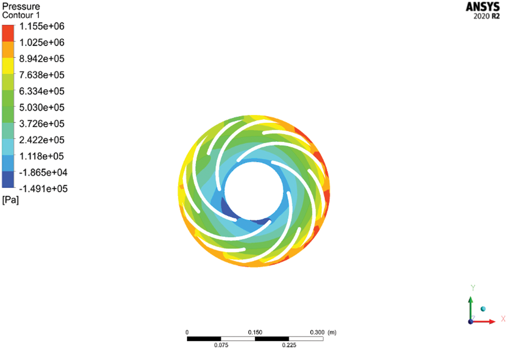
Figure 20: Impeller pressure cloud map after optimization

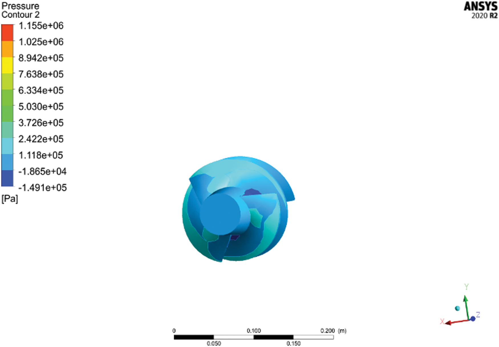
Figure 21: Inducer pressure cloud map after optimization

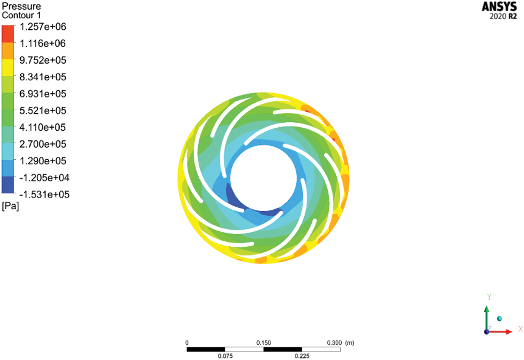
Figure 22: Impeller pressure cloud diagram before optimization

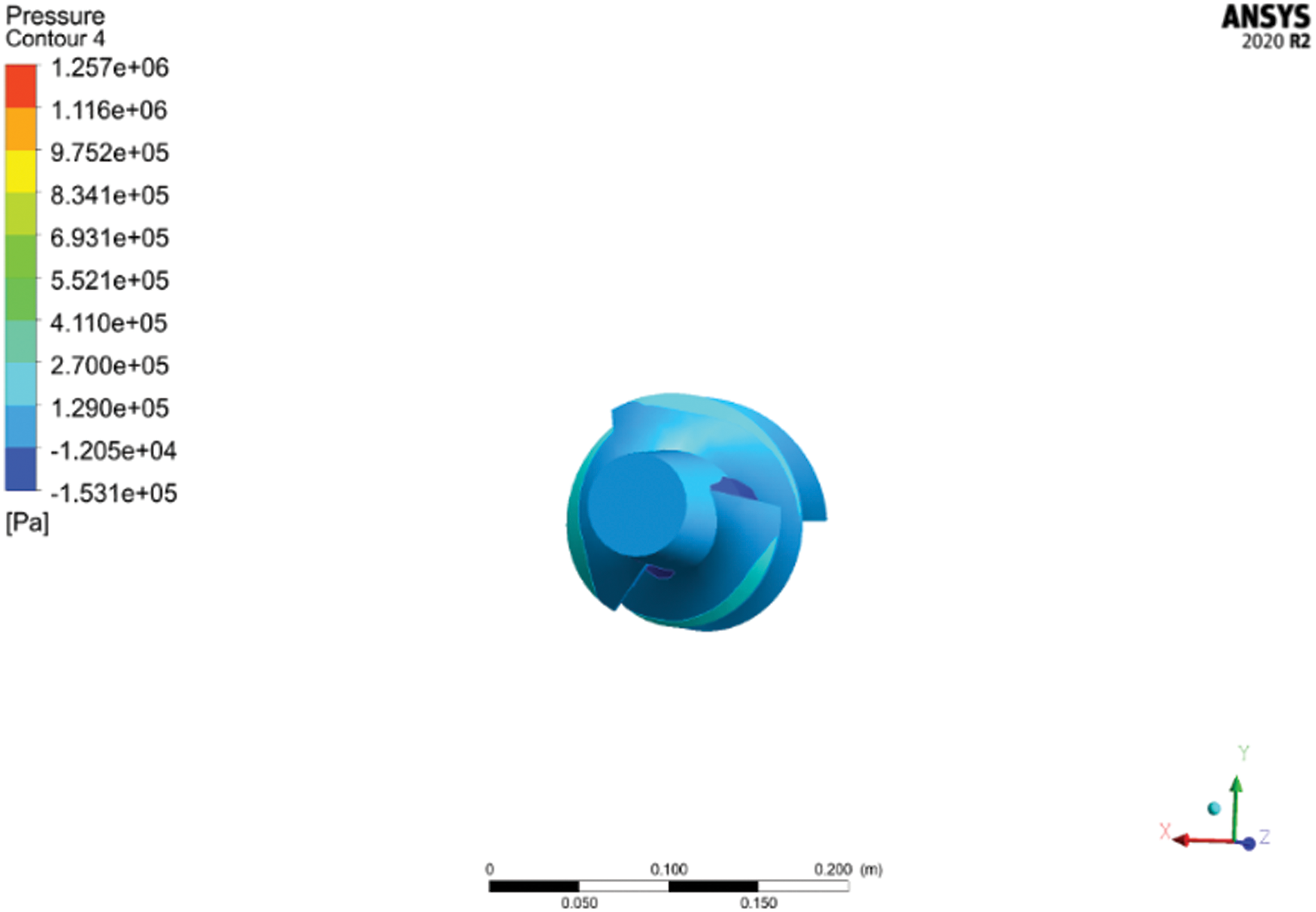
Figure 23: The pressure cloud map of the inducer before optimization

As can be seen from Table 9, different quality index values were obtained using orthogonal tests and least squares and fish swarm based algorithm analysis to optimize the plastic centrifugal pump inducer structural parameters. The head and shaft power obtained from the analysis based on least squares and fish swarm algorithms are not optimal among the three sets of quality evaluation index data mentioned above, but they are taken into account for both head and shaft power. Therefore, it is also verified that the least squares and fish swarm based algorithms are useful for optimizing the structural parameters of the plastic centrifugal pump inducer.

6  Conclusion

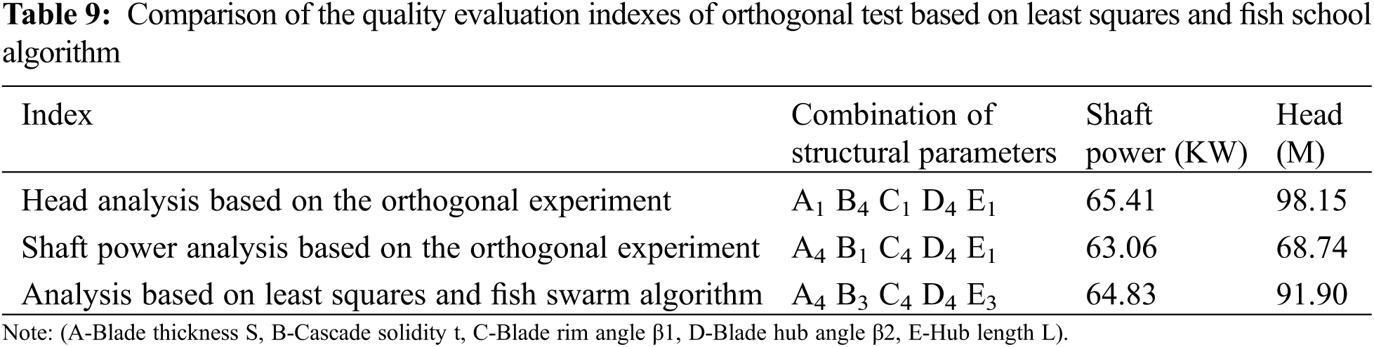
(1)   In this paper, L16 (165) orthogonal experiment table is designed. The influence of each factor on the shaft power of plastic centrifugal pump is in descending order: cascade solidity > blade rim angle > hub length > blade thickness > blade hub angle. The best combination of parameters under the condition of shaft power is: A4 B1 C4 D4 E1, the minimum shaft power can be obtained when that the inducer blade thickness is 5 mm, the cascade solidity is 1.6, the blade rim angle is 252°, the blade hub angle is 350°, the hub length is 140 mm. The influence of each factor on the head of the plastic centrifugal pump is, in descending order, cascade solidity > blade rim angle > hub length > blade hub angle > blade thickness. The best combination of parameters for the head condition is: A1 B4 C1 D4 E1, i.e., The maximum head can be obtained when the inducer blade thickness is 2 mm, the cascade solidity is 2, the blade rim angle is 235°, the blade hub angle is 360° and the hub length is 140 mm.

(2)   Using based on least squares and fish swarm algorithm to optimize the multi-objective optimization with the minimum shaft power as the optimization objective, the optimal combination of parameters of the plastic centrifugal pump inducer is obtained: A4 B3 C4 D4 E3, that is, inducer blade thickness is 5 mm, cascade solidity is 1.9, blade rim angle is 252°, blade hub angle is 360°, hub length is 145 mm, and the combination has the greatest impact on the head and shaft power. has the greatest impact.

(3)   The head and shaft power obtained by CFX analysis of the optimized model are 91.90 m and 64.83 KW, respectively. the head and shaft power obtained by applying the least squares and fish swarm algorithms are not optimal among the three sets of quality evaluation index data, but both the head and shaft power are taken into account. Therefore, it is known that the least squares and fish swarm algorithms are useful for optimizing the structural parameters of the plastic centrifugal pump inducer.

Funding Statement: This article belongs to the project of the “The University Synergy Innovation Program of Anhui Province (GXXT-2019-004)”, “Natural Science Research Project of Anhui Universities (KJ2021ZD0144)”, “Wuhu Key R&D Project: Research and Industrialization of Intelligent Control Method of Engine Energy-Feeding Hydraulic Semi-Active Mount”.

Conflicts of Interest: The authors declare that they have no conflicts of interest to report regarding the present study.

References

1. Guan, X. (2009). Modern pump theory and design, pp. 241–298. Beijing, China: China Aerospace Press. [Google Scholar]
2. Pasini, A., Torre, L., Cervone, A., d’Agostino, L. (2011). Continuous spectrum of the rotordynamic forces on a four bladed inducer. Journal of Fluids Engineering, 133(12), 121101. DOI 10.1115/1.4005258. [Google Scholar] [CrossRef]
3. Wang, W., Chen, H., Li, Y., Du, Y. J. (2015). Matching between inducer and centrifugal wheel of high-speed centrifugal pump. Journal of Drainage and Irrigation Mechanical Engineering, 33(4), 301−305. [Google Scholar]
4. Wu, G., Yang, J., An, C. (2017). Research on the influence of inducer on the performance of aviation fuel centrifugal pump. Gansu Science Journal, 29(3), 73–76. [Google Scholar]
5. Shojaeefard, M. H., Hosseini, S. E., Zare, J. (2019). CFD simulation and pareto-based multi-objective shape optimization of the centrifugal pump inducer applying GMDH neural network, modified NSGA-II, and TOPSIS. Structural and Multidisciplinary Optimization, 60, 1509–1525. DOI 10.1007/s00158-019-02280-0. [Google Scholar] [CrossRef]
6. Kang, B. Y., Kang, S. H. (2015). Effect of the number of blades on the performance and cavitation instabilities of a turbopump inducer with an identical solidity. Journal of Mechanical Science and Technology, 29, 5251–5256. DOI 10.1007/s12206-015-1126-6. [Google Scholar] [CrossRef]
7. It, Y., Tsunoda, A., Nagasaki, T. (2015). Experimental comparison of backflow-vortex cavitation on pump inducer between cryogen and water. Journal of Physics Conference Series, 656(1), 012063. DOI 10.1088/1742-6596/656/1/012063. [Google Scholar] [CrossRef]
8. Tani, N., Yamanishi, N., Tsujimoto, Y. (2012). Influence of flow coefficient and flow structure on rotational cavitation in inducer. Journal of Fluids Engineering, 134(2), 021302. DOI 10.1115/1.4005903. [Google Scholar] [CrossRef]
9. Cheng X, R., Liu, H., Tu Y, X. (2018). Effect of inducer sweepback on cavitation performance of centrifugal pump. IOP Conference Series: Earth and Environmental Science, 163(1), 012107. DOI 10.1088/1755-1315/163/1/012107. [Google Scholar] [CrossRef]
10. Sun, Q. Q., Jiang, J., Zhang, S. S., Chen, Q. (2017). Effects of variable pitch inducer on cavitation performance of high-speed centrifugal pumps. Journal of Drainage and Irriga-tion Machinery Engineering, 35(10), 856–862. [Google Scholar]
11. Kang, D., Watanabe, T., Yonezawa, K. (2010). Inducer design to avoid cavitation instabilities. American Institute of Physics, 433–446. DOI 10.1063/1.3464890. [Google Scholar] [CrossRef]
12. Furukawa, A., Ishizaka, K., Watanabe, S. (2001). Experimental study of cavitation induced oscillation in helical inducer with various blade lengths. Transactions of the Japan Society of Mechanical Engineers Series B, 67, 2425–2430. DOI 10.1299/kikaib.67.2425. [Google Scholar] [CrossRef]
13. Kim, S., Choi, C., Kim, J. (2013). Tip clearance effects on cavitation evolution and head breakdown in turbo pump inducer. Journal of Propulsion Power, 29(29), 1357–1366. [Google Scholar]
14. Cheng, X., Liu, X., Lv, B. (2022). Influence of the impeller/guide vane clearance ratio on the performances of a nuclear reactor coolant pump. Fluid Dynamics & Materials Processing, 18(1), 93–107. DOI 10.32604/fdmp.2022.017566. [Google Scholar] [CrossRef]
15. Parikh, T., Mansour, M., Thévenin, D. (2022). Maximizing the performance of pump inducers using CFD-based multi-objective optimization. Structural and Multidisciplinary Optimization, 65(1), 1–23. DOI 10.1007/s00158-021-03108-6. [Google Scholar] [CrossRef]
16. Shojaeefard, M. H., Hosseini, S. E., Zare, J. (2019). CFD simulation and pareto-based multi-objective shape optimization of the centrifugal pump inducer applying GMDH neural network, modified NSGA-II, and TOPSIS. Struct. Structural and Multidisciplinary Optimization, 60(4), 1509–1525. DOI 10.1007/s00158-019-02280-0. [Google Scholar] [CrossRef]
17. Zhang, Y. (2019). Research on the influence of the blade placement angle of the plastic centrifugal pump on the pump performance based on fluid-structure coupling. Wuhu, China: Anhui Polytechnic University. [Google Scholar]
18. Le, Z. (1985). Design and research of low specific speed pump. Pump Technology, 10(4), 1–4. [Google Scholar]
19. Zhu, Z., Wang, L. (1996). Empirical design of low specific speed and high-speed compound impeller centrifugal pump. Fluid Machinery, 24(2), 18–21. [Google Scholar]
20. Chebanowski (1997). Cavitation characteristics of high-speed inducers. Pump Technology, 6(3), 1–17. [Google Scholar]
21. Wang, F. (2004). Computational fluid dynamics analysis, pp. 136–196. Beijing, China: Tsinghua University Press. [Google Scholar]
22. Li, X., Yuan, S., Pan, Z. (2012). Realization and application evaluation of boundary layer grid for centrifugal pumps. Journal of Agricultural Engineering, 28(20), 67–72. [Google Scholar]
23. Gu, C., Li, D., Chen, S. (2012). Methods of mathematical physics, pp. 236–296. Beijing, China: Higher Education Press. [Google Scholar]
24. Liang, X., Zhao, J. (2019). Application of artificial fish swarm and genetic hybrid algorithm in path planning of unmanned boat. Computer Engineering and Science, 41(5), 942–947. [Google Scholar]
25. Li, X., Fang, L. (2016). Infrared image segmentation based on two-dimensional renyi entropy and adaptive artificial fish swarm algorithm. Ship Electronics Engineering, 36(7), 109–113. [Google Scholar]
26. Fei, O. (2020). Research on port logistics distribution route planning based on artificial fish swarm algorithm. Journal of Coastal Research, 115(sp1), 78–80. DOI 10.2112/JCR-SI115-023.1. [Google Scholar] [CrossRef]
27. Bi, L. (2015). Hybrid optimization algorithm based on artificial fish swarm and particle swarm algorithm. Engineering of Surveying and Mapping, 15(2), 763–777. DOI 10.1007/978-3-642-31346-2_68. [Google Scholar] [CrossRef]
28. Du, T., Hu, Y., Ke, X. (2015). Improved quantum artificial fish algorithm application to distributed network considering distributed generation. Computational Intelligence and Neuroscience, 2015, 851863. DOI 10.1155/2015/851863. [Google Scholar] [CrossRef]
29. Ma, X., Liu, N. (2014). Artificial fish swarm algorithm with adaptive vision to solve the shortest path problem. Journal of Communications, 35(1), 1–6. [Google Scholar]
30. Neshat, M., Sepidnam, G., Sargolzaei, M. (2014). Artificial fish swarm algorithm: A survey of the state-of-the-art, hybridization, combinatorial and indicative applications. Artificial Intelligence Review, 42, 965–997. DOI 10.1007/s10462-012-9342-2. [Google Scholar] [CrossRef]
Cite This Article
Copyright © 2023 The Author(s). Published by Tech Science Press.
This work is licensed under a Creative Commons Attribution 4.0 International License , which permits unrestricted use, distribution, and reproduction in any medium, provided the original work is properly cited.
Downloads
Citation Tools