Performance of a Phase Change Material Battery in a Transparent Building

1  Introduction

The demand for low-energy buildings has encouraged the development of new technologies for Heating, Ventilation, and Air Conditioning (HVAC). In this sense, thermal batteries seem to be ideal for dealing with variable heat sources once the systems reach a steadier operation level to save energy [1]. In buildings, PCMs could fulfill that role; and they have been mostly employed for thermal control in roofs [2], floors [3], and walls [4]. Moreover, PCMs have also been considered for space cooling [5], solar chimneys [6], PV/T (Photovoltaic/Thermal) modules [7], and residential electricity production [8], and heat exchangers [9–12]. Among the materials, Calcium Chloride Hexahydrate has a satisfactory cost-benefit balance and, more importantly, has no fire risk like the paraffin-based PCMs [13,14]. Additionally, nanoparticles have promised to suppress relevant drawbacks, such as the salt’s low thermal conductivity and degree of sub-cooling [15].

The literature shows various applications in the built environment sector. However, the focus of most of this literature is on liquid/PCM heat-exchangers, and studies utilizing three phases, gas, liquid, and solid, are somewhat more limited. Much literature on liquid/PCM heat-exchangers evaluates the effect of surface-enlargement like with the addition of fins [16,17]. The analyses reported by other workers generally compare numerical and experimental approaches [18]. Nevertheless, there is no consensus in the literature about the best numerical approach since it depends on the system configuration. Some authors have validated models considered in commercial software [19] and the coupling of software, e.g., CFD (computational fluid dynamics) with EnergyPlus [20]. Furthermore, some studies suggest that the PCM’s hysteresis is still a hurdle and requires more attention [21,22]. A fast overview of air-PCM applications based on IEA- and Solar Decathlon-research is given in [10,23].

This article focuses on using a PCM in a vertical air-handling unit with Heating, Ventilation, and Air Conditioning (HVAC) in a climate tower. This tower was originally designed as a thermal chimney in which the PCM is used as a buffer to reduce temperature fluctuations of the lightweight building itself [24]. The performance of the PCM battery is evaluated experimentally and theoretically. The experimental measurements are carried out in the battery with a high air-flow capacity (3 kg/s) and 18 Negative Temperature Coefficient (NTC) sensors, which are used to validate the simulation results. These are obtained from CFD simulations performed using PHOENICS, a Fortran-based CFD tool [25], and a simplified model for system control and optimization, implemented in MATLAB [26]. The accuracy of the models is validated, and the effect of simplifications and PCM hysteresis are investigated. Furthermore, we analyze the system performance under the flow-rate constraints and the demand for heating and cooling. The experimental setup and theoretical approaches are presented in Sections 2 and 3, respectively, while the results, plate temperatures, load times, and the models’ variance are discussed in Section 4. Conclusions and directions for future research are provided in Section 5.

The aim of the research is to investigate to what extent it is possible to model the existing PCM-battery and how it can be integrated in the building as a whole. CFD is used to get a better understanding of the fundamental background of the physical processes and is a reference for the MATLAB-model. With the MATLAB-model calculation time can be reduced, the energy savings over a whole year can be evaluated and an integration of the model with all the relevant components of the building is possible to find the most optimal control strategy.

2  Starting Points of the PCM Battery Design

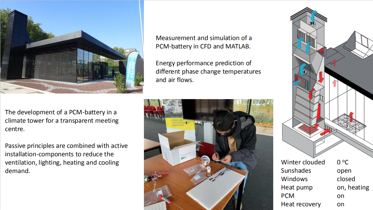
The building in which the battery is applied is around 315 m2 and is designed to be as transparent as possible for a passive building with active components (see Figs. 1a and 1b). The façade is made of triple glazing, and is the main framework of structural glass. The building has dynamic outdoor sunshades and is largely heated by solar irradiation, internal heat generation from people, and electrical devices like computers. Cooling is provided mainly by outdoor air. As the building can be occupied by many individuals (e.g., 130–240 people), cooling via PCMs and a heat pump is sometimes necessary. The PCM and the heat pump also provide heat in winter. The PCM battery and heat pump are installed in the climate tower, as shown in Figs. 1c and 1d, via which the fresh supply air is generally passing through a counter-flow heat exchanger. The comfort requirements of the building are realized firstly by natural sources like the sun and outdoor air (e.g., rooftop windows), secondly by mechanical air supplied via the heat exchanger and/or the PCM battery, and finally by the heat pump.

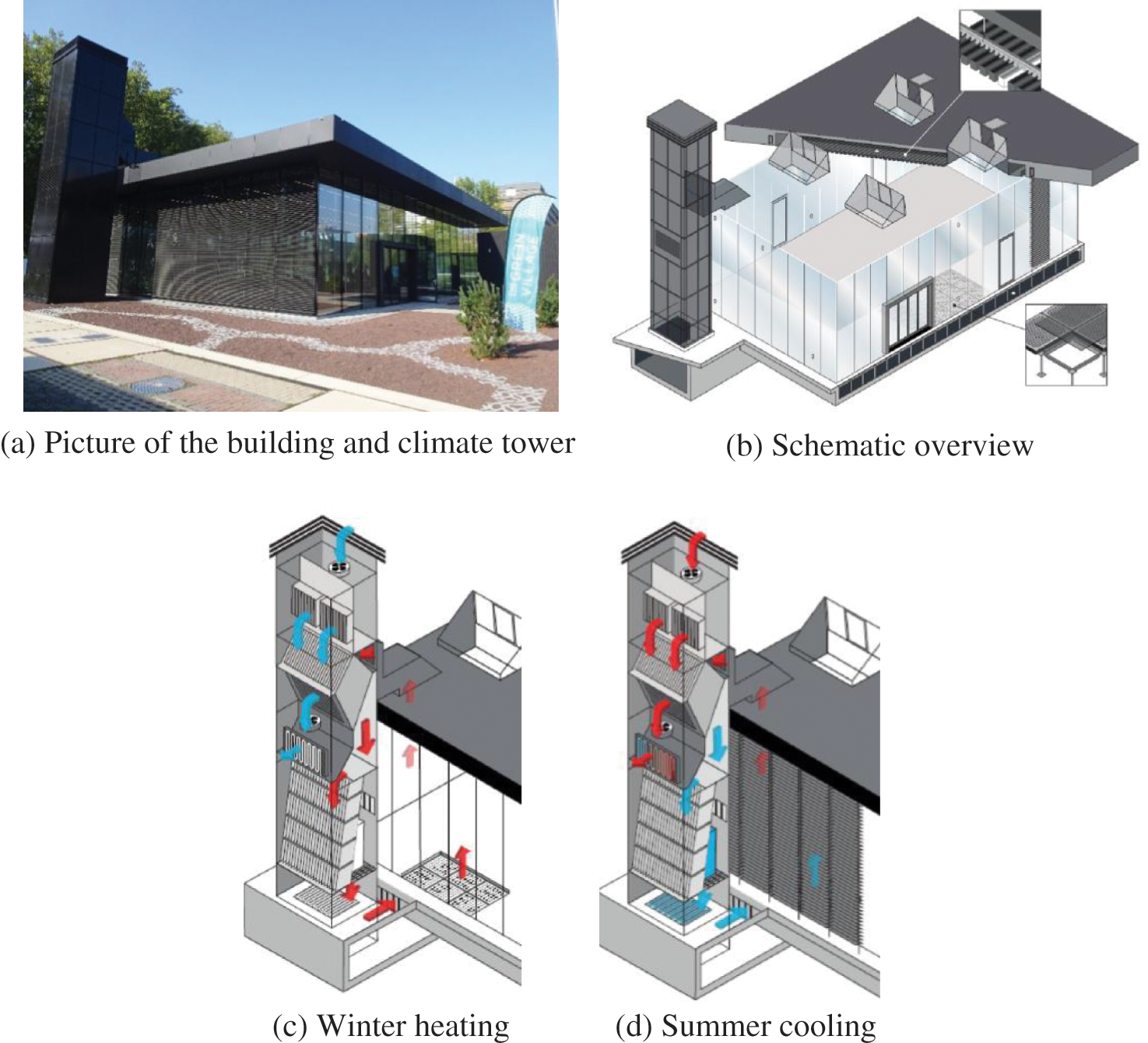
Figure 1: (a) Real picture and (b) schematic overview of the building and climate tower, with illustrations for (c) winter heating and (d) summer cooling operation modes

The thermal battery has 2,106 kg of PCM in the climate tower with a minimum cooling and heating power of 7.2 kW. The storage capacity of the PCM is 181 kWh (18.5 m3 natural gas equivalent). Additionally, the heat pump has a nominal cooling power of 30 kW and heating power of 15 kW. This analysis is presented in Fig. 2. With a capacity of 7.2 kW, the PCM battery could deliver most of the heating and a large part of the cooling demand. However, in practice, it is still tricky to load the PCM with sufficient heat because of the lack of solar heat in winter. As for the cooling load in summer, the temperature of the nights should be sufficiently low. The PCM battery is distributed across 1,170 PCM panels, each with 275 × 570 × 13 mm dimensions and stacked inside the climate tower, as illustrated in Fig. 3. Between each of the 1,170 PCM panels, there is a free space of 4 mm, through which the airflow is driven by forced convection. The total free space area is circa 1.29 m2, and so a maximum airflow of 10,800 m3/h produces an air velocity of 2.3 m/s between each panel.

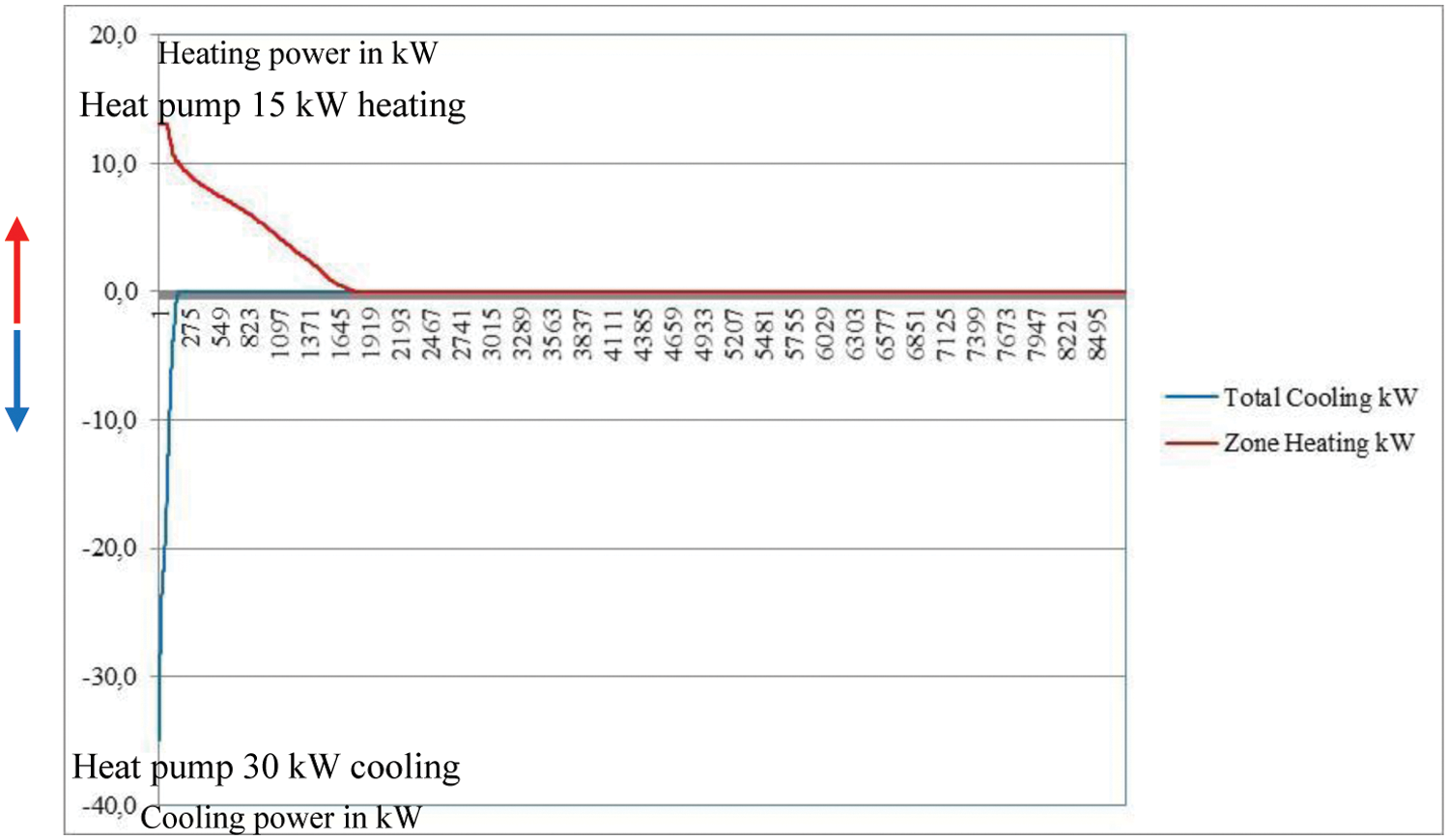
Figure 2: Heating and cooling demand and potential capacity of the PCM and the heat pump. The calculation has been executed in DesignBuilder for the year 2021 and the weather station of Rotterdam

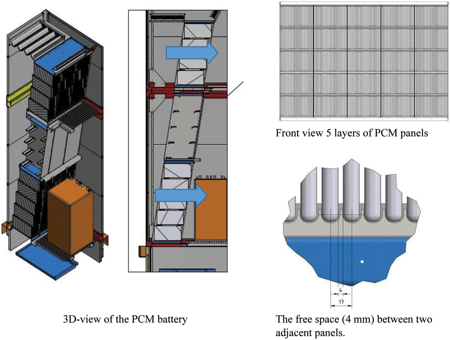
Figure 3: Configuration of the PCM battery (1,170 panels)

Some (unforeseen) limiting parameters for the airflow are stated below:

•   The noise level from the fans should not exceed 40 dB(A) according to the Dutch building code. The high-efficiency EBM-Past fans (VBH0450PTTLS K3G450-PAA23-71) in the climate tower have a source noise of 87.6 dB(A) at 8,000 m3/h, so the maximum airflow is limited by this fan choice. The high noise level is produced mainly by a valve and the fans having too small a free-flow surface area. This leads to a very high maximum velocity of 37 m/s via the fans, a high measured pressure difference of circa 2,500 Pa, and unnecessary high electrical-energy consumption. This could be solved by replacing the fans with lower-velocity fans using a maximum velocity of 10 m/s. However, the current fan noise produced at 10,800 m3/h is still acceptable to the building owner. This amount of air is only used with a very high occupancy of 240 people in a reception-like meeting. During such a meeting, with the fans producing an indoor sound level of 49.2 dB(A), the noise of talking people is comparable. During the day, for this laboratory-like location, a 55 dB(A) noise level at a distance of 40 m is still acceptable to the people living in the surrounding environment. The main problem is not the noise level in general but a disturbing sharp, so-called Aeolian sound via a grille or by the PCM battery. The Aeolian sound is already present at velocities below three m/s, the maximum air velocity via the valve. It is not clear yet how to solve this problem.

•   The minimum airflow for operating the heat pump is limited to prevent malfunction. Thus, the airflow via the fans cannot be reduced below circa 3,500 m3/h. This will be solved by connecting the heat pump to energy storage in the ground in the near future.

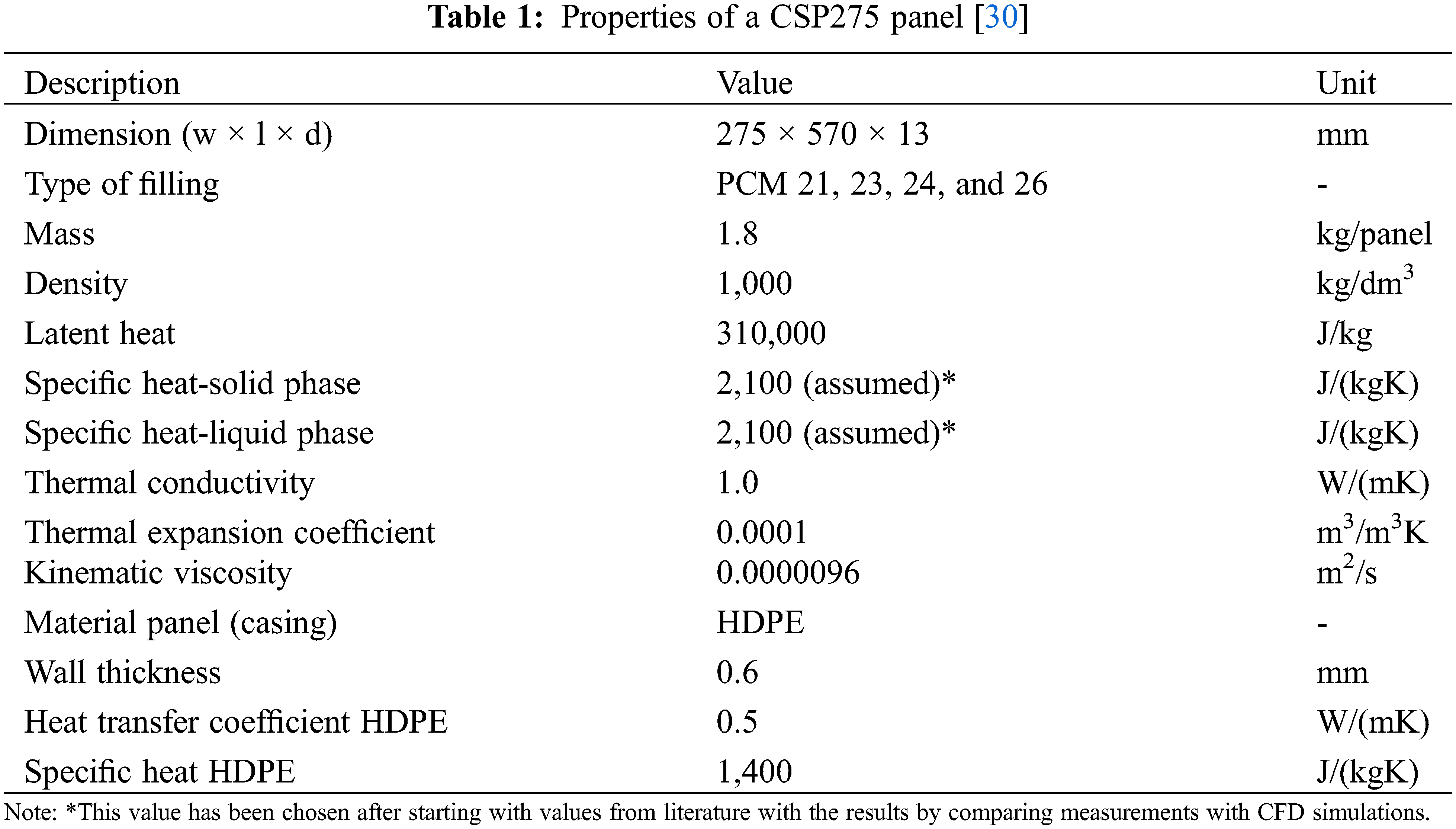
The material in the panels is Calcium Chloride Hexahydrate, which is encapsulated within Crystal Storage Panels (CSP) made of HDPE (high-density polyethylene) material, as shown in Fig. 4. The melting temperature of the PCM is between 20°C and 23°C (Fig. 5), and the total storage capacity depends on the density of material in the panel. In this case, the panels have a salt density that is 1.8 times greater than the density in kg/m3 for the one shown in Fig. 5; and they have a mole fraction of approximately 0.4% of CaCl2 by weight [27]. The total thermal storage capacity of the panel, associated with phase change, is calculated as 310 kJ/kg. The overall properties of the panel are presented later on in Table 1.

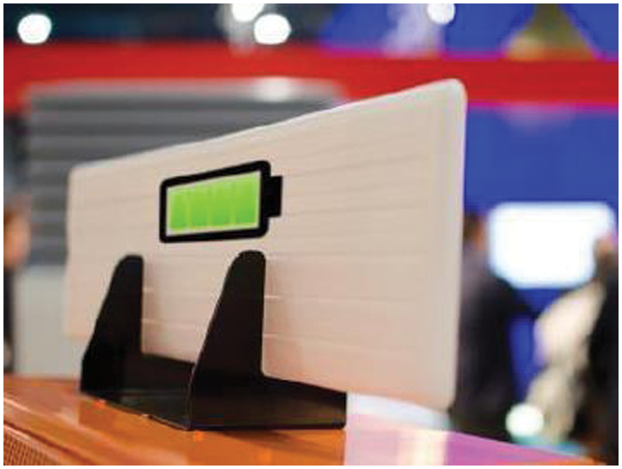
Figure 4: Impression of a PCM in a single crystal storage panel (CSP275). As visible, the panel is divided into 6 semi-closed sections

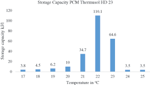
Figure 5: Phase-change profile of a PCM with a melting and solidification zone between 20°C and 23°C, and a total storage capacity of 172 kJ/kg. A PCM with a total storage capacity of 310 kJ/kg is used here

3  Methods and Models

3.1 General

Three approaches are used to evaluate the PCM battery performance. First, the temperature of the PCM panels is evaluated experimentally, relying on the set of sensors installed in situ, as described in Section 3.2. Later, a set of numerical simulations are developed using the CFD tool PHOENICS and MATLAB, which are detailed in Sections 3.3 and 3.4, respectively.

3.2 Measurements

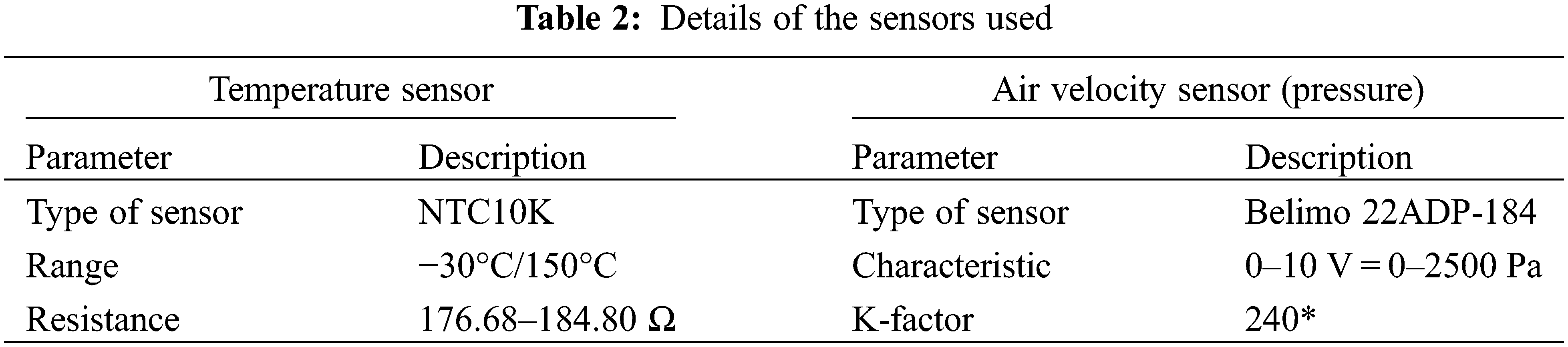
The PCM surface, supply, and exhaust air temperatures are measured, as are the air flow rate and relative humidity. These are collected at 5-min intervals by a set of sensors installed in the system. Additionally, temperature sensors are installed at the inlet and outlet of each sub-system, such as the heat exchanger, the PCM battery, and the heat pump. The specifications of the installed temperature and air velocity sensors and their operational features are listed in Table 2.

The air velocity is calculated from the pressure difference and the K-factor, which is defined by

q=ΔPK ∗3600 (1)

where q is the volumetric flow rate in m3/h. For instance, with a K-factor of 240 and a pressure difference of 40.1 Pa, the airflow q is 1,471 m3/h. In K the flow area and air density ρ are included, which is a limitation of the accuracy of this equation.

The 1,170 panels in the PCM battery are divided into two decks separated by a metallic plate, and panels fill the unused third deck with a lower phase-change temperature. The temperature of the PCM battery is measured with 18 sensors, of which 9 are located on the upper deck and 9 on the lower deck. The temperature sensors are placed within the 4 mm gap between the panels in each deck. The sensors are located to facilitate the temperature profile measurement over the entire PCM battery, as shown in Fig. 6c. On the panels located in the center, there are five sensors to verify the surface temperature profile on a single plate, as shown in Fig. 6a. The influence of air temperature on the measurements is reduced by isolating the temperature sensors from the airflow with Polyurethane (PU) foam, as shown in Fig. 6b. While this isolation prevents, to some extent, the direct flow of air over the sensors, it does not completely prevent the sensors from measuring the air temperature. Hence, a marginal error in measuring the actual PCM panel temperature is to be expected, as will be elaborated on further in Section 4.2. Two additional temperature sensors are placed at the positions marked as ‘X’ in Fig. 6c: one at the inlet and the other at the outlet of the PCM battery. These sensors measure the air temperature before and after it passes through the battery.

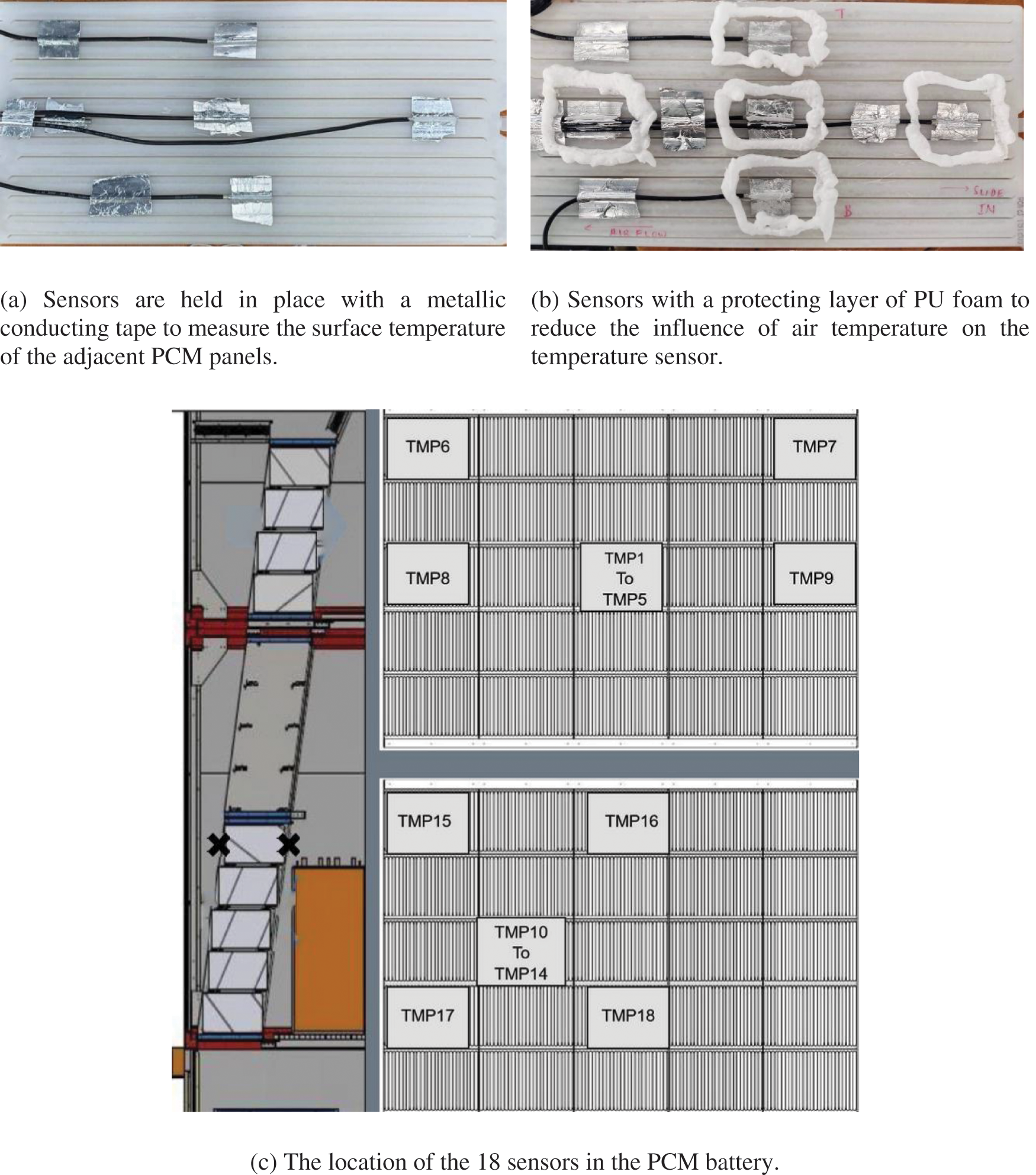
Figure 6: Temperature sensor locations in the PCM battery and centrally-located panels

The overall temperature of the PCM battery is calculated by taking an average of the measurements provided by the 18 sensors. The measured data are provided in real-time by a monitoring interface that can be accessed online through its corresponding website (see Fig. 7). The flow rate readings from the building management system (BMS) are used to calculate the inlet velocity for the CFD model.

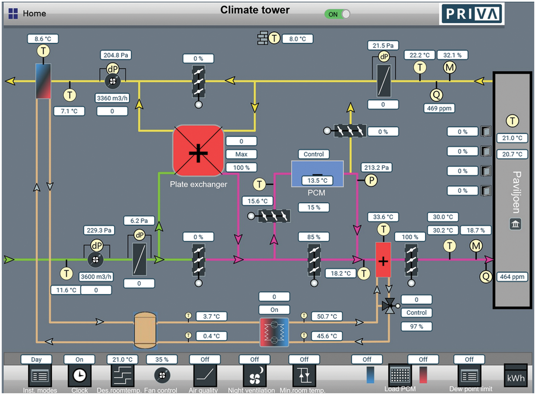
Figure 7: An overview of the BMS interface, the PCM battery is presented by the central blue box

3.3 CFD Model

3.3.1 Mathematical Model

A transient, three-dimensional CFD model of the PCM battery is developed using the general-purpose CFD code PHOENICS to solve the conservation equations for mass, momentum and energy. The battery comprises the liquid and solid regions of the PCM which are housed within solid casings, and these in turn undergo conjugate heat transfer with the air flow in the adjacent channels. The PCM’s undergo melting and solidification processes with natural convection in the melt, and they are modelled using the enthalpy-porosity formulation of Voller et al. [28], but with the use of an effective specific heat capacity for the treatment of the latent-heat evolution. A similar approach was adopted for transparent facades by Tenpierik et al. [29].

3.3.2 Physical Properties

In the air channels between the PCM panels, the following uniform values are used for the physical properties of air: k = 0.023 W/mK, Cpa = 1,005 J/kgK, ρ = 1.189 kg/m3 and ν = 1.154.10−5 m2/s. Table 1 presents the properties of the PCM panel used in the simulations.

3.3.3 Discussion on the Heat Transfer Coefficients

The temperature difference between the PCM panel and the air and the convective heat transfer coefficient ( hc ) are the main parameters that determine the time needed to load or unload the PCM panel. For internal flow, the overall convective heat-transfer coefficient is defined as

hc=NukD (2)

where Nu is the Nusselt number, k is the thermal conductivity of the air, and D is the hydraulic diameter for internal flow. This defines the overall heat transfer coefficient, as do Eqs. (3) to (6) below. Transport phenomena literature [31] can find correlations between laminar and turbulent air flows in ducts.

For laminar flow, the following expressions are in use for making estimates of the heat transfer coefficient:

Nu=1.62Re0.33Pr0.33(dD)−0.33,whenax⟨v⟩D2<0.05 (3)

Nu=3.66ifax⟨v⟩D2>0.1 (4)

where Re is the Reynolds number, Pr is the Prandtl number, and d is the distance between the surface and fluid. In the case of a turbulent regime, when Re > 5722 [32] and Pr ≥ 0.7, the model considers the following expression:

Nu=0.027Re0.8Pr0.33 (5)

However, even at Reynolds numbers as low as 800, perturbations in the channel flow can initiate a transition to a turbulent regime [33]. Hence, assuming a turbulent airflow already with a Reynolds number of 1,053, at 2 m/s, and hydraulic diameter of 0.00784 m, a Prandtl number of 0.713 at 20°C and k of 0.023 W/mK, the hc value can be calculated as 18.3 W/m2K. A high convective heat transfer coefficient can lead to a rapid rise in the air temperature in the cavity. When the airflow is laminar, the hc value is much lower, for instance, 10.2–10.8 W/m2K.

The value of hc , halfway through the (un)loading process, can also be estimated at an early stage. With a constant velocity of 2 m/s, a supplied air temperature of 15°C and a peak wall temperature of 23°C, the following energy balance can be used

hc=V˙ρcΔTtotal/((Apcm,surface)(Tinlet−Tpcm,highest2)) (6)

With 100% heat transfer efficiency and assuming a linear rise of temperature in the cavity, the convective heat transfer coefficient from a steady-state CFD simulation is calculated as hc = 16.8 W/m2K. This hc -value lies between the expected values for laminar (10.2 W/m2K) and turbulent (18.3 W/m2K) flow.

3.3.4 Turbulence and Standard-Wall Function

Turbulence is ignored in the PCM melt, whilst the Chen-Kim k-ε model [34] is employed in the air channels together with a standard wall-function treatment [35]. The latter ensures that if the near-wall grid node lies in laminar flow or in the turbulent flow regime, Fourier’s law is employed so that the local heat transfer coefficient hc = k/δ where δ is the wall-to-node distance. Suppose the near-wall flow is in the turbulent regime, then the local heat-transfer coefficient is computed from a wall function, so that hc = St ρ Ur Cp where Ur is the near-wall air velocity and St is the local Stanton number, which is computed from a modified Reynolds analogy [35].

3.3.5 CFD Solution Method

The foregoing mathematical model has been incorporated into the general-purpose, commercial CFD code PHOENICS for solution on a structured Cartesian grid using a finite-volume numerical method. Fully implicit backward differencing is employed for the transient terms and central differencing for the diffusion terms. The convection terms are discretized using hybrid differencing [36] where these terms are approximated by central differences, which is second-order accurate, if the cell face Peclet number Pe < 2 and by upwind differences, which are first-order accurate, if Pe > 2. At faces where the upwind scheme is used, physical diffusion is omitted altogether.

The set of finite volume equations are solved iteratively using the SIMPLEST [37] algorithm, which is a variant of the well-known SIMPLE algorithm [38]. These are segregated solution methods which employ pressure-velocity coupling to enforce mass conservation by solving a pressure-correction equation and making corrections to the pressure and velocity fields. Many iterations are conducted until convergence is attained at the current time level, and the pressure-correction equation is solved in a simultaneous whole-field manner at the end of each iteration. Thereafter the solution proceeds to the next time level where the iterative process is repeated.

The numerical solution procedure requires appropriate relaxation of the flow variables in order to procure convergence. Two types of relaxation are employed, namely inertial and linear. The former is normally applied to the velocity variables, whereas the latter is applied to all other flow variables, as and when necessary.

The convergence requirement is that for each set of finite volume equations the sum of the absolute residual sources over the whole solution domain is less than 1% of reference quantities based on the total inflow of the variable in question. An additional requirement is that the values of monitored dependent variables at a selected location do not change by more than 0.1% per cent between successive iteration cycles.

3.3.6 Conservation Equations

The continuity and momentum equations for each fluid phase can be written in generic form as follows:

∂ρ∂t+∇.(ρU)=0 (7)

∂(ρU)∂t+∇.(ρUU)=−∇p++ ∇.τ+Sg+Sm (8)

where ρ is the density, τ is the viscous stress tensor, p the pressure, U the velocity vector, Sg is a momentum source term representing the effects of gravity, and Sm is a flow resistance term which is zero in air space and given by Eq. (13) below in the melt. In the air channels, gravitational effects are negligible, so Sg = 0; whereas Boussinesq’s approximation is used within the melt so that Sg = ρgβΔT, where g is the gravity vector, β is the coefficient of thermal expansion, and ΔT is the temperature difference between the local and reference temperature. This means that uniform densities are used in both the melt and the air space, but the foregoing equations are written in generic form to reflect the flexibility of the PHOENICS implementation.

The energy equation for both fluid and solid regions can be written as follows:

∂(ρh)∂t+∇.(ρUh)=∇.(k∇T) (9)

where h refers to the specific enthalpy, k the thermal conductivity, and T the temperature. In solid regions, U = 0 so that convection is absent. The enthalpy-temperature relationship of the PCM is defined in the next section; and within the air space and solid casings, h = CpT, where Cp is the specific heat capacity of the air or solid.

3.3.7 PCM Modelling

The PCM considered is Calcium Chloride Hexahydrate, and this is represented in the CFD model by employing a linear phase-change equation, where the evolution of latent heat is expressed as a linear function of temperature based on an effective specific heat capacity corresponding to the estimated solid fraction. Therefore, the specific enthalpy h, at temperature T, is expressed as follows:

h=∫0T⁡CpdT+(1−fs)L (10)

where L is the latent heat of the material, fs the solid fraction, and Cp the effective specific heat capacity, given by:

Cp=fsCps+(1−fs)Cpl (11)

where Cps is the solid-phase specific heat capacity, and Cpl is the liquid-phase specific heat capacity. The solid fraction, fs , at temperature T, is calculated according to the Scheil-Gulliver equation [39]:

T≤Ts:fs=1

Ts<T<Tl:fs=(Tl−T),(Tl−Ts) (12)

T≥Tl:fs=0

where Ts is the solidus temperature and Tl is the liquidus temperature. The partially-solidified region is treated as a porous medium and the porosity in each mesh cell is defined in terms of the solid fraction fs , which is equal to unity in fully solidified regions. A flow resistance term is then introduced into the momentum equations to reduce the PCM-liquid velocities in partially-solidified regions, and suppress them completely in fully solid regions. The resistance term is based on the Kozeny-Carman equation for a porous medium, and takes the following form:

Sm=−(ρCfs2vi)/[E+(1−fs)3] (13)

where Sm is the momentum volumetric force vector, ρ the melt density, vi the velocity vector, C is a constant equal to 106 which controls the degree of velocity damping and E is a small number equal to 0.001 to prevent division by zero.

3.3.8 Computational Details, Spatial and Temporal Discretization Study

The final solution domain for the CFD simulations consists of one complete panel at the center and two half panels on either side. The mesh used for the domain consists of 30 cells in the X direction, 36 cells in the Y direction, and 20 cells in the Z direction, as illustrated in Fig. 8. The chosen mesh is selected after a mesh-sensitivity study. Further, within the solution domain, two 4 mm wide cavities are included on either side of the central panel. To reduce the computational time, a smaller section of the panel of l × w × h = 0.57 × 0.036 × 0.05 m is used in the final simulations. This approaches the size of a compartment within a panel. Since the actual height of the panel is 0.275 m, the results from the CFD predictions are used to calculate the overall heat transfer coefficient associated with the entire PCM battery. For verification, the temperature from the simulations with the original panel dimensions is compared with the results of this smaller panel. The two simulations show the same temperature trends, affirming the validity of the approach. The casing of the PCM is modeled as glass with a conductivity comparable to 0.0006 m of HDPE.

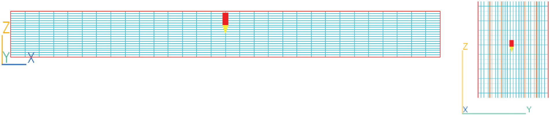
Figure 8: CFD grid for simulation of the PCM battery

The simulation settings used for the final CFD simulations in PHOENICS are summarized in Table 3. A summary of spatial and temporal grid studies are illustrated in Tables 4 and 5, respectively. The Grid Convergence Index (GCI) is calculated for different grid refinement ratios in the range 1.5 to 2 along X, Y and Z directions, by considering the lowest value among the respective values. The observed order of convergence is taken as a conservative estimate of unity. The evaluating parameters, temperature of the PCM (TPCM) and the temperature of the outlet air (TAir) are chosen to calculate the errors. The values imply good grid independence given that the GCI is less than 9% for coarse grids and less than 3% for fine grid given that the refinement ratio is in the range 1.5 to 2 [40]. Furthermore, the number of cells within the PCM and in the air channels were varied along the Y direction independently. Through this, it is noted that the values of Tair are much more sensitive than the values of TPCM which is clearly reflected in their respective GCI. For the temporal convergence a constant refinement ratio of 2 is considered and the observed order of convergence is calculated to be 1.23. The GCI here, is also calculated to be within permissible limits. All the values of GCI are calculated with a conservative factor of safety of 3. It is noted that the simulation is sensitive to large fluctuations in temperature and velocity (seen in Fig. 9). Hence the temperature and velocity input data are averaged over a span of 30 min to smoothen the abrupt changes caused by the errors in measurements. The number of time steps and the number of the inner iterations for each are chosen with care to achieve convergence with the fluctuation in the input data. Finally, to ensure convergence of the simulation, the values of the local and global residuals are obtained at intervals of 10 time steps, and these were observed to be below 0.1%. Furthermore, the values of velocity and temperatures from the simulations were observed at a single monitoring point across the entire time duration and the largest variations were found to be within 3% of the computed value.

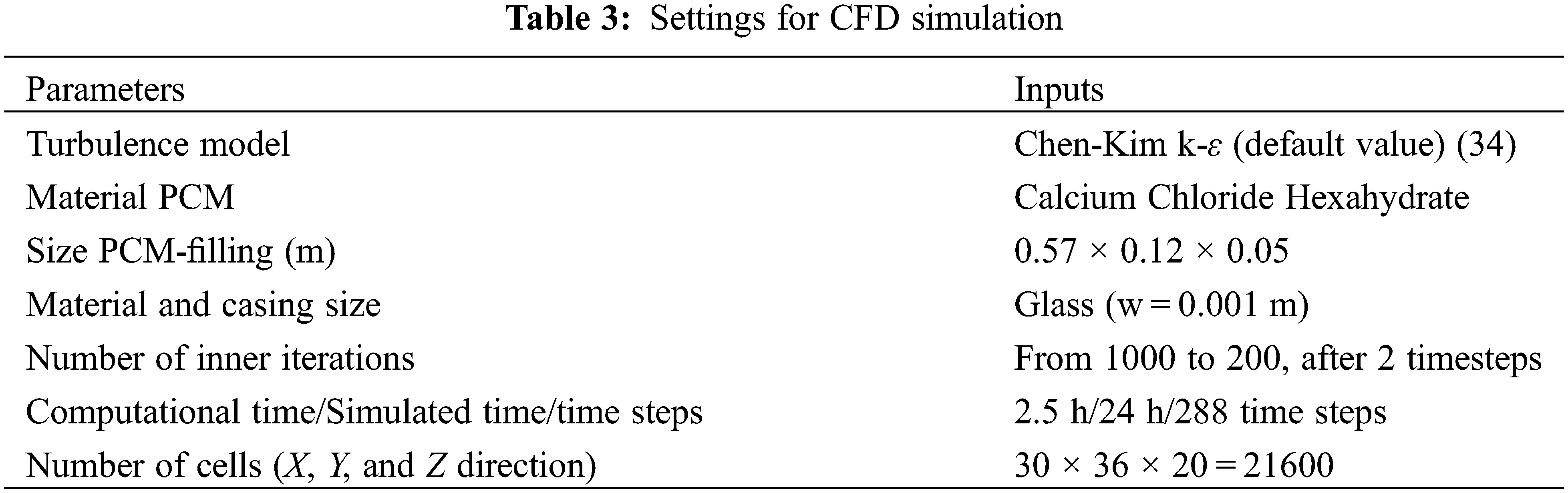
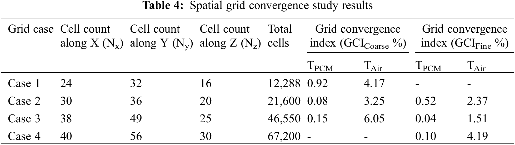
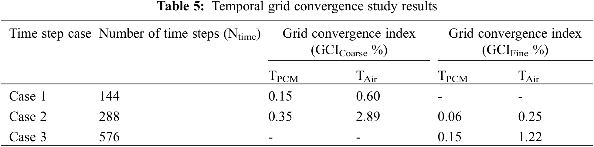
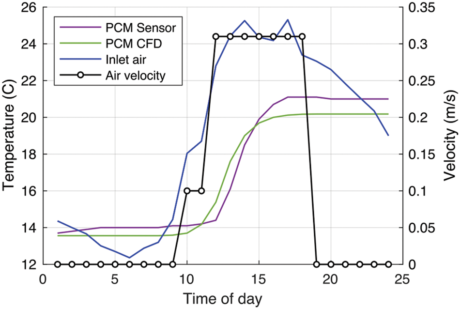
Figure 9: Hourly-averaged values from measurements (on 30-03-2021) and CFD simulations of the model with an increased number of cells of Fig. 8

3.4 MATLAB Model

The CFD simulations can be time-consuming for performing dynamic tasks. Therefore a flexible, dynamic model was implemented in MATLAB for integration into optimization algorithms used for developing control strategies. Such modeling essentially reduces the conservation Eqs. (7) to (9) to a one-dimensional transient system by making simplifications, such as ignoring effects like buoyancy, heat losses, and friction while assuming incompressible, one-dimensional flow. The convective heat transfer between the airflow and the PCM plates is determined from Eqs. (2) and (5). Moreover, the model assumes a lumped capacitance approach for transient conduction and, similar to the CFD-simulations, disregards any irradiation heat exchanges. Furthermore, the MATLAB model does not consider the HDPE case enclosing the PCM plates.

3.4.1 Mathematical Model

The control volume, which is here defined as the battery volume, is discretized into three subsections in the flow direction x. At each time interval t, the temperatures of the airflow at the downstream nodes (Ta,x+1t) and PCM plates (Tp,xt) at can be determined by applying Eq. (14) for the air and plates volume in each subsection x. Therefore, disregarding the thermal capacity of the air, the energy balance considers the change in the advective flow rate equivalent to the convective heat exchange between the air and PCM plates, such that the 1d quasi steady-state formulation for the airflow is determined as

(m˙aCa+hcA2)Ta,x+1t+(hcA2−m˙aCa)Ta,xt−(hcA)Tp,xt=0forx=1…3 (14)

where m˙a is the airflow rate, Ca the specific heat of air, and A the heat transfer area. Similarly, when dealing with PCM plates, their thermal capacity is taken into account so that the energy balance considers that the convective heat transfer between the plates and the air is equivalent to the variance in the amount of heat stored in the plates. When there is no phase change, i.e., the PCM plates are in the solid state or the liquid state, the following equation describes the transient 1d-energy balance for the PCM:

(hcA2)Ta,x+1t+(hcA2)Ta,xt−(hcA+MpCpΔt)Tp,xt=(−MpCpΔt)Tp,xt−1forx=1…3 (15)

where Mp is the mass of PCM, Cp is the specific heat of PCM, and Δt is the time step of integration. On the other hand, during the phase transition period (i.e., when Tp,xt is between 20°C and 23°C), the energy balance additionally accounts for the solid fraction fs,xt and the latent heat stored in the PCM plates. Hence, the corresponding equations for calculating the temperatures of fluid (Ta,x+1t) and PCM plates (Tp,xt) are determined by the 1d-energy balance for air and PCM, respectively, as follows:

(m˙aCa+hcA2)Ta,x+1t+(hcA2−m˙aCa)Ta,xt=(hcA)Tp,xt−1forx=1…3 (16)

(hcAΔt2MpCp)Ta,x+1t+(hcAΔt2MpCp)Ta,xt−(hcAΔtMpCp)Tp,xt−(1−fs,xt)=−(1−fs,xt−1)forx=1…3 (17)

Note that in contrast to Eqs. (14) and (16) assumes an explicit discretization as a simplification, in which the PCM-temperature for convective heat transfer with the air is taken as the temperature at the previous time step ( Tp,xt−1 ). For closing the balance, the system considers Eq. (12) for calculating fs,xt while considering α=1 , such that the fraction of solid in each discretization node is expressed as

Tp,xt+3fs,xt=23forx=1…3 (18)

The system of equations above, i.e., Eqs. (14)–(18), is implemented and solved in MATLAB, during the time interval [0, t Δt ]. The results of these simulations are discussed in Section 4 below.

4  Results and Analysis

4.1 General

The results produced by the CFD and MATLAB models are compared with those of experiments. The analysis shows that with an assumed constant high enthalpy in the phase change (20°C–23°C) period, a good prediction of the loading/unloading time can be made. In the following paragraphs, the results are discussed.

4.2 CFD Model

The accuracy of the CFD model is evaluated by considering the PCM temperatures obtained numerically and experimentally. Such an analysis is based on a time horizon of 24 h, each hour denoting the average of 12 measurements carried out every 5 min. During this time interval, the temperature and velocity of the air entering the PCM battery (as shown in Fig. 9) are specified at the inlet boundary of the CFD simulations. These values are obtained from the measurements provided by the Building Management System on a real-time basis, as measured on March 30, 2021. The initial temperature of the supplied air and PCM panels is 13.5°C. The temperature sensors only measure the surface temperature of the PCM along the X and Z directions at 5 points. The internal temperature of the PCM along the Z direction cannot be measured without compromising the panel’s integrity, and so it is not taken into consideration. Since the temperature of the PCM panel is not the same along the X, Y, and Z directions, an average value of the temperature was taken by averaging the PCM temperature across all the cells within the central panel. This average temperature of the panel is compared with that of the PCM battery, which is the average of the 18 sensors in Fig. 6c. As seen in Fig. 9, both curves show the same trend. The measurement curve shows that the PCM temperature rises rather fast even at velocities lower than 0.31 m/s and the CFD results reaffirm this observation. However, the temperature curve of the PCM panel obtained from the simulations seems to under-predict the phase transition temperature by 1°C when compared with the measurements. This difference can be explained with the following reasoning:

•   The PCM is modeled with a linear phase change, as described by the Scheil-Gulliver equation, between 20°C to 23°C. Whereas the phase change in the PCM is non-linear with the maximum phase change occurring at 22°C (see Fig. 5).

•   Although the temperature sensors are isolated with PU foam, some influence of the air temperatures on the panel temperature sensors is expected. This leads to the temperature sensors measuring a marginally different temperature than its actual value.

•   Finally, the simulation average is calculated, including the inner temperatures of the PCM, while the measurements only consider the surface temperatures of the panel.

Another noticeable deviation of the CFD results from the measurements can be seen in the time interval between 02:00 and 10:00; where the CFD predicts a uniform trend in the PCM temperature, whereas the measurements show a marginal increase during this period. It is to be noted that the measured temperatures rise despite the decreasing inlet air temperature during the period mentioned above (see Fig. 9). This can be attributed to the influence of the heat pump on the PCM battery and a marginal error in the lower limit of the flow-rate measurement sensor. Despite these deviations, the study indicates an accurate prediction of the trends by the CFD model in comparison with the measured temperature, with a marginal error of 4.7%. Hence, the CFD model can be considered validated against the measurements and can be used to evaluate the PCM battery’s performance.

The performance of the PCM battery is evaluated by using a steady inflow rate of air at three different uniform inlet velocities: 0, 8, 1.5, and 2.3 m/s, and a constant inlet temperature of 15°C. However, a fixed inlet temperature cannot be realized in the battery. This is why the validation is derived from simulations of a “real-life” working pattern, as in Fig. 9. The results are summarized in Table 6.

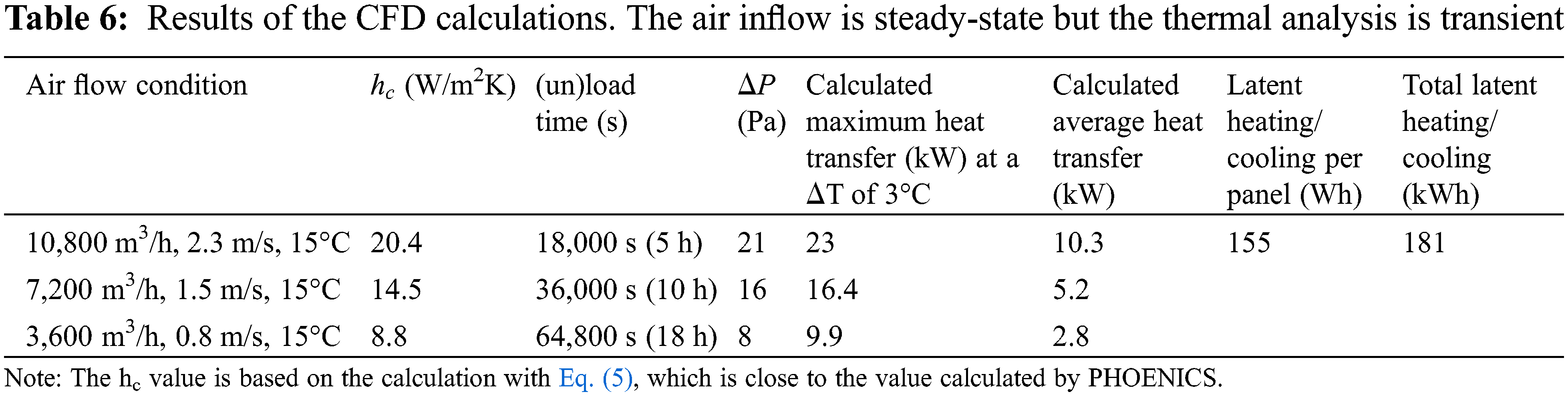
The study shows that initially, the heating and cooling capacity of the PCM battery is higher than the nominal power of the PCM battery (stated as 7.2 kW) and then becomes lower with time, depending on the inlet air velocity and temperature. Another observation from this study is that the buoyancy effect used in the CFD model of the PCM shows a minimal influence on the temperature profile of the PCM panel. This highlights that even at low or zero flow rate, the effects of natural convection in the air channel, on the temperature profile of the PCM panels can be ignored. Finally, it can be seen from Table 6 that even a low air velocity of 1 m/s is sufficient to heat or cool the building when combined with the heat pump (when necessary). The importance of this is twofold: apart from the noise reduction, the axis-power of the fan P is proportional to the third root of the rotational frequency N (or the airflow) of the fan. The equation relating the axis power with the rotational frequency is as follows:

P1P2=N13N23 (19)

Therefore, in theory, the electrical power of a fan for an air velocity of 1 m/s will be, theoretically, 23 = 8 times lower than for a velocity of 2 m/s. However, in practice, the difference will be much smaller in practice due to energy losses.

Finally, temperature contours at a central plane of the PCM panel are shown in Fig. 10, where each plot is displayed at a different time step (t = 61,200 s to t = 86,400 s). These temperature profiles are simulated for the night-cooling period of the 10th of August using air conditions for a peak summer day in Delft. The yellow zone identifies temperatures above 20°C, so one can see the phase-change front (i.e., the yellow zone) getting cooler with time. The buoyancy effect can also be seen in the contours with a larger quantity of warmer PCM mass at the top of the panel, and a colder mass at the bottom. Consequently, the rate of solidification inside the PCM is higher at the bottom, while the melting rate is higher at the top of the panel. Fig. 10 also highlights that the phase change is not spatially uniform, which brings up the challenge of measuring these temperatures. In reality, the panel is divided into six semi-closed compartments (see Fig. 4), and so the temperature distribution will differ.

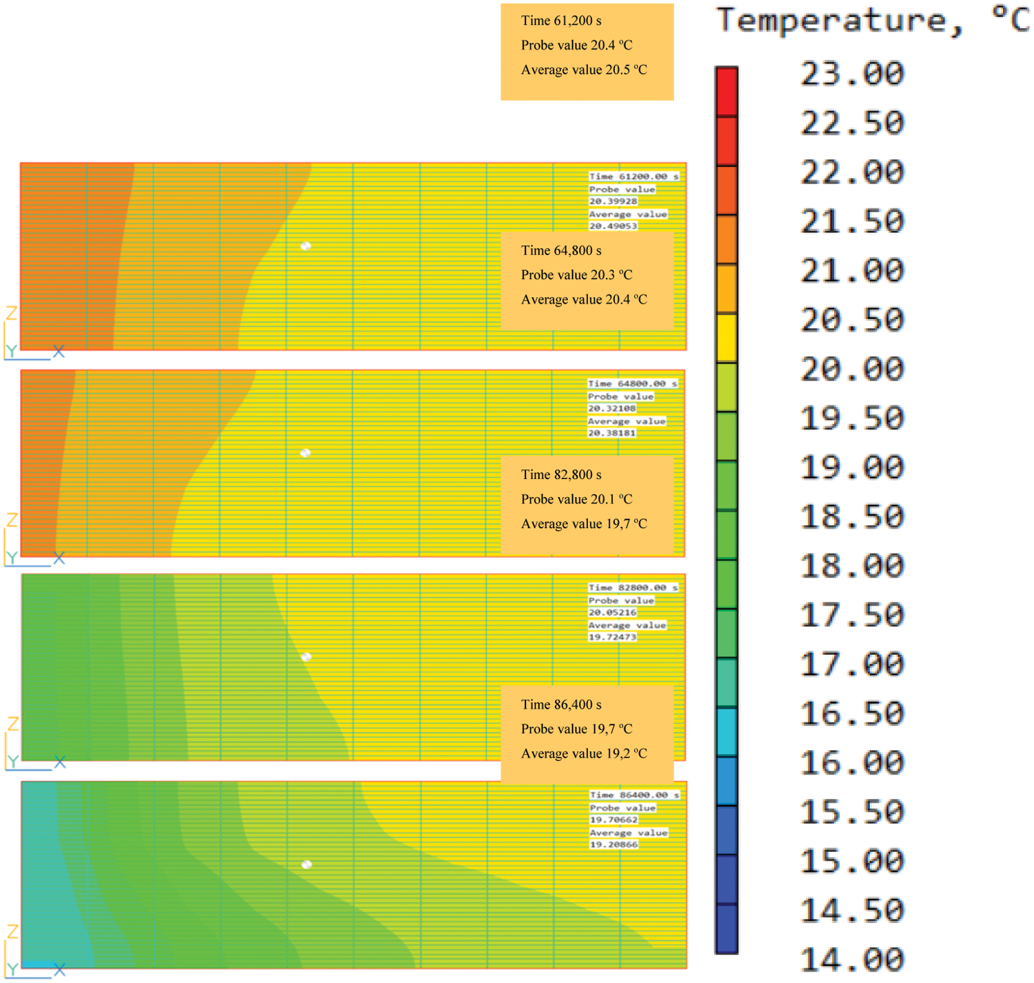
Figure 10: Contour plot of temperature at the core of PCM panel obtained from the CFD simulations, the panel is simulated as one compartment here

The numbers of cells x-, y- and z-direction are: 10, 36, 40 (14,400) here. For the final simulations in Table 6, the CFD model of Fig. 8 is used, where the total number of cells is increased in a smaller circa-1/6 section of the panel: 30, 36, 20 (21,600).

For this model, an additional grid-refinement evaluation has also been executed. The maximum numbers of cells in this evaluation are x = 60, y = 56 and z = 30. The effect of increasing the number of cells can be neglected, as also could be concluded by comparing the MATLAB and CFD calculations in Fig. 11.

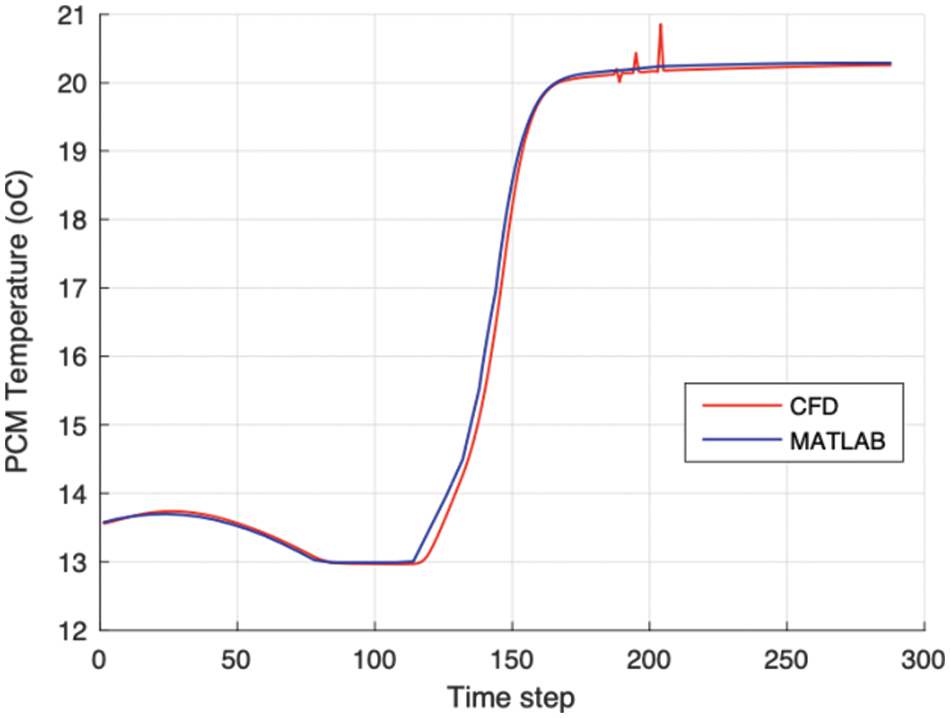
Figure 11: Temperature of the PCM plates calculated in CFD (red) and MATLAB (blue) using the same input data

4.3 MATLAB Model

In Fig. 11, the PCM-temperatures calculated in MATLAB are compared with CFD (PHOENICS, with the model of Fig. 10), and the resemblance between both numerical approaches is evident. The temperatures show an almost perfect agreement throughout the entire time interval. The minimal differences displayed over the heating period from time step 120 to 160 can be attributed to the simplifications made in the MATLAB model, such as lumped capacitance, one-dimensional flow, and no casing. Nevertheless, the temperature profiles shown in Fig. 11 demonstrate that the numerical implementation is consistent and exempt from major mistakes, as suggested by the code-to-code validation.

Next, we compare the temperatures obtained in MATLAB against the sensor measurements extracted from a different time horizon, which was recorded on December 02, 2021. First, Fig. 12 presents the measured airflow and temperatures, which were used at the inlet boundary of the MATLAB simulation.

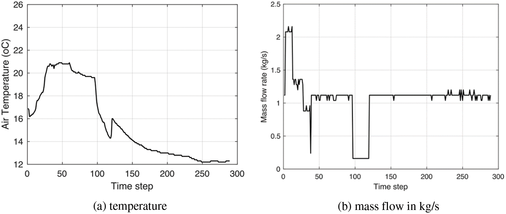
Figure 12: Input data recorded on December 02, 2021

The strange peak in the CFD simulation values after 200 time-steps has a relation with the warm supplied air at that moment (see Fig. 9). This is probably related to using too coarse a grid.

The PCM temperatures calculated in MATLAB are displayed in Fig. 13 where the temperatures read by the sensors are also shown (green curve). The MATLAB predictions are similar to the experimental measurements, which indicates the accuracy of the numerical approach. Such fair agreement is also reflected in the variance, which reveals an average value of 2.4% and a maximum of 10%. The slight discrepancy shown during charge and discharge is a consequence of the simplifications, such as constant latent heat and the correlations used for the heat transfer coefficient. Moreover, the phase-change period in MATLAB happens before the sensor measures this. For instance, between the time steps 50 and 100, the sensor data in Fig. 13a shows temperatures that surpass the melting temperature of 20°C, while the MATLAB data adhere to this value; this occurs because the sensor measurements record the air temperature on the actual PCM surface, resulting in a sensible thermal storage behavior. The effect is illustrated and verified in Fig. 13b, where the predicted PCM temperatures are those for when the phase change only starts from 21°C. The MATLAB curve shown in the figure replicates the sensor measurements better between time steps 50 and 100. On the other hand, the latent thermal storage indicated in time steps 100–120 is not reached, in contrast to the MATLAB curve shown in Fig. 13a, which induces a more severe decay when operating in discharge mode. The variance-accounted-for, in this case, is slightly higher, yielding an average of 2.9% and a peak of 12.8%.

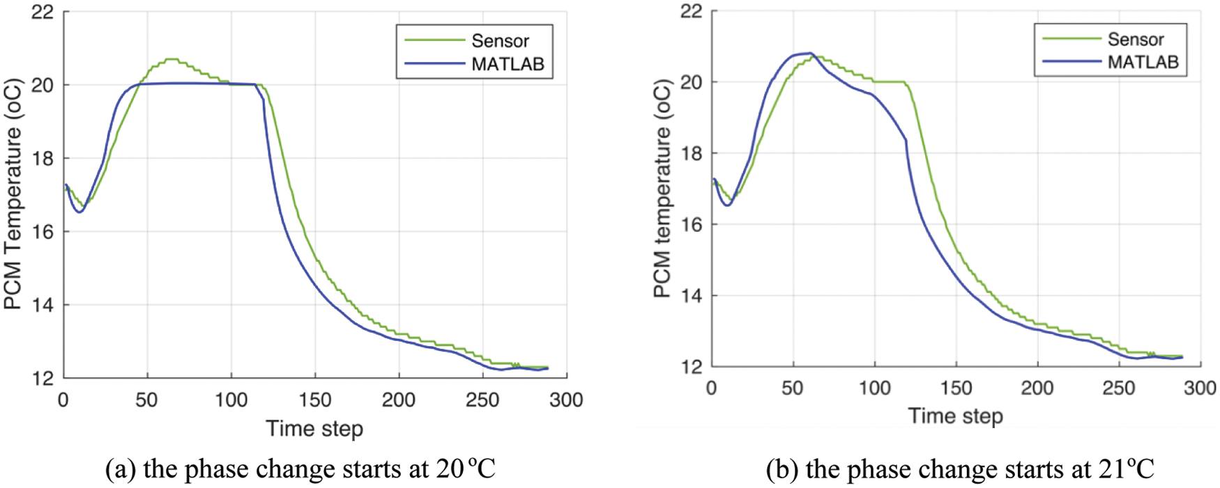
Figure 13: PCM temperatures from MATLAB and sensor measurements (December 02, 2021), considering a melting temperature of 20°C (a) and 21°C (b)

After assessing the conformity between numerical and experimental results, we now employ the MATLAB model to evaluate the PCM-battery performance over different conditions while extrapolating scenarios with full charge/discharge periods. Such conditions depend on weather conditions rarely reached in the building in winter, such as, for example, an inlet air temperature >23°C. Therefore, an initial condition where the PCM battery is fully charged is assumed. At a PCM temperature of 23°C, the discharge time depends on the airflow through the PCM and the inlet air temperature, as shown in Fig. 14. The mapping shows that the discharge takes between 2 to 50 h, depending on the airflow conditions. The message in Fig. 14 is that at lower air temperatures, a higher ΔT , the system may operate at lower flow rates and that the discharge time can be kept in the magnitude of 2 to 15 h (blue zone). Higher inlet temperatures are more sensitive to a drastic increase in flow rate, in which the discharge time can change from 10 to 50 over the same operation range.

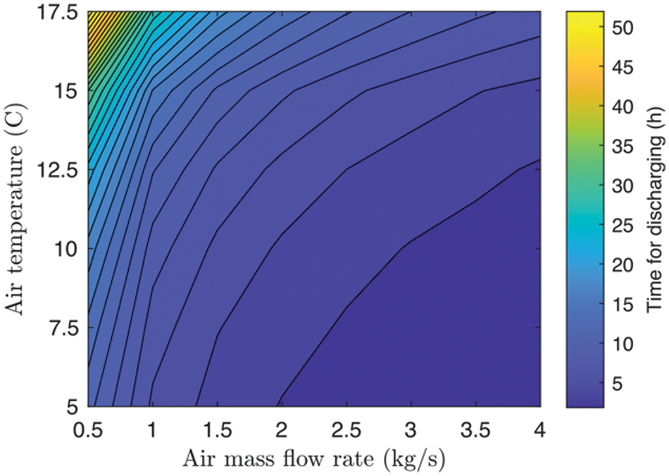
Figure 14: Discharge time as a function of the mass flow rate and inlet temperature of the supply air

5  Conclusions and Future Research

The dynamic behavior of a PCM battery, designed for buffering part of the energy demand, is investigated experimentally and numerically. The measurements use 18 sensors distributed over the system and provide the PCM-temperature profile over 5-min intervals. Numerical data are available from CFD (PHOENICS) and MATLAB simulations.

The following conclusions can be drawn:

•   A PCM-based heat exchanger can be designed for air preheating and cooling in climate systems of large office buildings.

•   The PCM battery, a composite of air/solid/liquid, can be simulated in CFD and MATLAB while predicting the loading and unloading times with a maximum variance of circa 10%.

•   The analyses show that the simulation-methods are comparable when evaluating the PCM-battery performance. The charge/discharge times are 2–50 h, depending on the inlet airflow rate (m3/h) and temperature differences.

•   The use of MATLAB as an addition to CFD reduces the calculation time and makes it possible to find an integrated solution. There is also a MATLAB-model developed for the whole building, so in this way it is possible to find the most optimal phase change temperatures.

•   The latent storage of the PCM can be simulated as a material with high enthalpy and to a considerable degree of accuracy. This shows that the effect of buoyancy or natural convection is low. This, and the limited effect of the grid size, has also been concluded by other researchers [12].

•   The heat transfer coefficient and specific latent heat play a major role when comparing numerical and experimental results. Further works are suggested to improve such correlation, including developing a grey-box model using Sequential Quadratic Programming to calibrate relevant system parameters [41].

•   The measured COP for cold and heat loading is circa 27 with the current fans operating at an airflow rate of 6.480 m3/h with an average ΔT of 6.5 K. For heating or cooling during occupancy time, the COP is much higher because the usage of fans is a part of the total system. The resistance of the battery with a maximum below 25 Pa is only a small percentage of the total system resistance. The fans themselves have a maximum flow already at a resistance of circa 2,500 Pa.

The following areas could become the subject of future research:

•   A low-pressure fan should be applied and the valve openings, and maybe the battery as well, should be designed in such a way that ventilation (and Aeolian) noise stays within an acceptable level at a much lower electrical energy consumption.

•   With a low-pressure ventilation system, the COP can become higher, above 100, considering the high current resistance of the current ventilation system.

•   Since the PCM battery is a low-pressure solution (<25 Pa), it can even be integrated into natural ventilation systems.

•   In the present building, a combination of PCMs with a heat pump connected to pipes in the ground (foundation pillars) will be applied soon. This will reduce the relevance of PCMs for cooling and heating, and this will also increase the general COP for heating from 2 to circa 5. Summer cooling by PCMs will reduce any unwanted warming up of the cold storage in the ground.

•   A main point of attention is how to load the PCM with sufficient warm air. In the current design, the availability of sufficient (passive solar) heat is very limited, especially in mid-winter.

•   A future option could be to load the PCM panels with heat from solar panels on the roof or to load the panels via the heat pump when there is a surplus of PV energy during the day.

•   More detailed simulations considering the material’s hysteresis (Fig. 5) will increase the accuracy of the CFD and MATLAB predictions.

•   The intention is to apply PCM batteries like this in other buildings. However, more insight into the added value of PCM batteries, often combined with heat pumps, is still necessary to be able to draw more detailed conclusions about the advantages and most optimal integration of such a system.

•   In the meantime more PCMs (1/3 of the total capacity) in the free part of the PCM battery (Fig. 6c) have been added. These PCMs have lower phase-change temperatures of 17°C–20°C. These return temperatures are more common in practice than 20°C–23°C and will reduce the energy-demand.

Acknowledgement: The PCM-battery and installations are designed and built by van Dorp B.V. (https://vandorp.eu/) and Orange Climate B.V. (https://www.orangeclimate.com/). Both companies have different locations in The Netherlands (see websites).

Funding Statement: The project is financed via a public grant of the Rijksdienst Voor Ondernemend Nederland (RVO, https://www.rvo.nl/) within the Urban Energy 2018 Research-Line with Grant No. TEUE318008. The grant is awarded to the following consortium: The Delft University of Technology (https://www.tudelft.nl/en), Van Dorp B.V., Hunter Douglas Europe B.V. (https://www.hunterdouglasarchitectural.eu/), Priva B.V. (https://www.priva.com/nl) and the Green Village Foundation (https://www.thegreenvillage.org/en/).

Conflicts of Interest: The authors declare that they have no conflicts of interest to report regarding the present study.

References

1. Cabeza, L. F., Chafer, M. (2020). Technological options and strategies towards zero energy buildings contributing to climate change mitigation: A systematic review. Energy and Buildings, 219, 110009. DOI 10.1016/j.enbuild.2020.110009. [Google Scholar] [CrossRef]
2. Lizana, J., de-Borja-Torrejon, M., Barrios-Padura, A., Auer, T., Chacartegui, R. (2019). Passive cooling through phase change materials in buildings. A critical study of implementation alternatives. Applied Energy, 254, 113658. DOI 10.1016/j.apenergy.2019.113658. [Google Scholar] [CrossRef]
3. Heng, W., Wang, Z., Wu, Y. (2021). Experimental study on phase change heat storage floor coupled with air source heat pump heating system in a classroom. Energy and Buildings, 251, 111352. DOI 10.1016/j.enbuild.2021.111352. [Google Scholar] [CrossRef]
4. Lamrani, B., Johannes, K., Kuznik, F. (2021). Phase change materials integrated into building walls: An updated review. Renewable and Sustainable Energy Reviews, 140, 110751. DOI 10.1016/j.rser.2021.110751. [Google Scholar] [CrossRef]
5. Chen, X., Zhang, Q., Zhai, Z., Ma, X. (2019). Potential of ventilation systems with thermal energy storage using PCMs applied to air conditioned buildings. Renewable Energy, 138, 39–53. DOI 10.1016/j.renene.2019.01.026. [Google Scholar] [CrossRef]
6. Jiménez-Xamán, C., Xamán, J., Moraga, N. O., Hernández-Pérez, I., Zavala-Guillén, I. et al. (2019). Solar chimneys with a phase change material for buildings: An overview using CFD and global energy balance. Energy and Buildings, 186, 384–404. DOI 10.1016/j.enbuild.2019.01.014. [Google Scholar] [CrossRef]
7. Yu, Q., Yu, Q., Chen, X., Yang, H. (2021). Research progress on utilization of phase change materials in photovoltaic/thermal systems: A critical review. Renewable and Sustainable Energy Reviews, 149, 111313. DOI 10.1016/j.rser.2021.111313. [Google Scholar] [CrossRef]
8. Violidakis, Ι, Zeneli, M., Atsonios, K., Strotos, G., Nikolopoulos, N. et al. (2020). Dynamic modelling of an ultra high temperature PCM with combined heat and electricity production for application at residential buildings. Energy and Buildings, 222, 110067. DOI 10.1016/j.enbuild.2020.110067. [Google Scholar] [CrossRef]
9. Morovat, N., Athienitis, A. K., Candanedo, J. A., Dermardiros, V. (2019). Simulation and performance analysis of an active PCM-heat exchanger intended for building operation optimization. Energy and Buildings, 199, 47–61. DOI 10.1016/j.enbuild.2019.06.022. [Google Scholar] [CrossRef]
10. Haghighat, F. (2014). Applying energy storage in ultra-low energy buildings-final report. ANNEX 31. DOI 10.13140/RG.2.1.4995.4727. [Google Scholar] [CrossRef]
11. Dardir, M., Panchabikesan, K., Haghighat, F., El Mankibi, M., Yuan, Y. (2019). Opportunities and challenges of PCM to air heat exchangers (PAHXs) for building free cooling applications–A comprehensive review. Journal of Energy Storage, 22, 157–175. DOI 10.1016/j.est.2019.02.011. [Google Scholar] [CrossRef]
12. Gholamibozanjani, G., Farid, M. (2019). Experimental and mathematical modeling of an air-PCM heat exchanger operating under static and dynamic loads. Energy & Buildings, 202, 109354. DOI 10.1016/j.enbuild.2019.109354. [Google Scholar] [CrossRef]
13. Tyagi, V., Buddhi, D. (2008). Thermal cycle testing of calcium chloride hexahydrate as a possible PCM for latent heat storage. Solar Energy Materials & Solar Cells, 92, 891–899. DOI 10.1016/j.solmat.2008.02.021. [Google Scholar] [CrossRef]
14. Rezvanpour, M., Borooghani, D., Torabi, F., Pazoki, M. (2020). Using CaCl2⋅6H2O as a phase change material for thermo-regulation and enhancing photovoltaic panels’ conversion efficiency: Experimental study and TRNSYS validation. Renewable Energy, 146, 1907–1921. DOI 10.1016/j.renene.2019.07.075. [Google Scholar] [CrossRef]
15. Wong-Pinto, L. S., Milian, Y., Ushak, S. (2020). Progress on use of nanoparticles in salt hydrates as phase change materials. Renewable and Sustainable Energy Reviews, 122, 109727. DOI 10.1016/j.rser.2020.109727. [Google Scholar] [CrossRef]
16. Mohamed, T., AjarosTagh, S. S. M., Yildiz, Ç., Arici, M., Kamal, A. et al. (2021). Performance enhancement of latent heat storage systems by using extended surfaces and porous materials: A state-of-the-art review. Journal of Energy Storage, 44, 103340. DOI 10.1016/j.est.2021.103340. [Google Scholar] [CrossRef]
17. Kahtra, L., Quarnia, H. E., Ganaoui, M. E. (2019). The effect of the fin length on the solidification process in a rectangular enclosure with internal fins. Fluid Dynamics & Materials Processing, 15(2), 125–137. DOI 10.32604/fdmp.2019.04713. [Google Scholar] [CrossRef]
18. Hu, Y., Heiselberg, P. K., Drivsholm, C., Søvsø, A. S., Vogler-Finck, P. J. C., Kronby, K. (2022). Experimental and numerical study of PCM storage integrated with HVAC system for energy flexibility. Energy and Buildings, 255, 111651. DOI 10.1016/j.enbuild.2021.111651. [Google Scholar] [CrossRef]
19. Wijesuriya, S., Tabares-Velasco, P., Biswas, K., Heim, D. (2020). Empirical validation and comparison of PCM modeling algorithms commonly used in building energy and hygrothermal software. Building and Environment, 173, 106750. DOI 10.1016/j.buildenv.2020.106750. [Google Scholar] [CrossRef]
20. Pandey, B., Banerjee, R., Sharma, A. (2021). Coupled EnergyPlus and CFD analysis of PCM for thermal management of buildings. Energy and Buildings, 231, 110598. DOI 10.1016/j.enbuild.2020.110598. [Google Scholar] [CrossRef]
21. Klimeš, L., Charvát, P., Mastani, J. M., Zálešák, M., Haghighat, F. et al. (2020). Computer modelling and experimental investigation of phase change hysteresis of PCMs: The state-of-the-art review. Applied Energy, 263, 114572. DOI 10.1016/j.apenergy.2020.114572. [Google Scholar] [CrossRef]
22. Zhou, Y., Zheng, S., Zhang, G. (2020). A review on cooling performance enhancement for phase change materials integrated systems—Flexible design and smart control with machine learning applications. Building and Environment, 174, 106786. DOI 10.1016/j.buildenv.2020.106786. [Google Scholar] [CrossRef]
23. Rodriguez-Ubinas, E., Ruiz-Valero, L., Vega, S., Neila, J. (2012). Applications of phase change material in highly energy-efficient houses. Energy and Buildings, 50, 49–62. DOI 10.1016/j.enbuild.2012.03.018. [Google Scholar] [CrossRef]
24. van den Engel, P. J. W., Bokel, R. M. J., Bembrilla, E., de Araujo Passos, L. A., Lucuere, P. G. (2022). Converge: Low energy with active passiveness in a transparent highly occupied building. Proceedings of CLIMA2022, Rotterdam, Netherlands. [Google Scholar]
25. CHAM: Experts in CFD Software and Consultancy, PHOENICS (2022). http://www.cham.co.uk/phoenics/d_polis/polis.htm. [Google Scholar]
26. MathWorks, MATLAB & Simulink (2022). https://mathworks.com/. [Google Scholar]
27. Farnam, Y., Dick, S., Wiese, A., Davis, J. M., Bentz, D. P. et al. (2015). The influence of calcium chloride De-icing salt on phase changes and damage development in cementitious materials. Cement & Concrete Composites, 64, 1–15. DOI 10.1016/j.cemconcomp.2015.09.006. [Google Scholar] [CrossRef]
28. Voller, V. R., Prakash, C. (1987). A fixed grid numerical modelling methodology for convection-diffusion mushy region phase-change problems. International Journal of Heat and Mass Transfer, 30, 709–1719. DOI 10.1016/0017-9310(87)90317-6. [Google Scholar] [CrossRef]
29. Tenpierik, M., Wattez, Y., Turrin, M., Cosmatu, T., Tsafou, S. (2019). Temperature control in (translucent) phase change materials applied in façades: A numerical study. Energies, 12, 3286. DOI 10.3390/en12173286. [Google Scholar] [CrossRef]
30. ISSO (2018). Phase change materials. Ontwerprichtlijn ten behoeve van klimatisering van gebouwen. ISSO-Publicatie 111. [Google Scholar]
31. van den Akker, H. E. A., Mudde, R. F. (1996). Fysische transportverschijnselen I. Delft: Delftse Universitaire Pers, Delft, Netherland. [Google Scholar]
32. Orszag, S. A. (1971). Accurate solution of the Orr–Sommerfeld stability equation. Journal of Fluid Mechanics, 50(4), 689–703. DOI 10.1017/S0022112071002842. [Google Scholar] [CrossRef]
33. Sano, M., Tamai, K. (2016). A universal transition to turbulence in channel flow. Nature Physics, 12(3), 249–253. DOI 10.1038/nphys3659. [Google Scholar] [CrossRef]
34. Chen, Y. S., Kim, S. W. (1987). Computation of turbulent flows using an extended k-e turbulence closure model. NASA CR-179204. [Google Scholar]
35. Launder, B. E., Spalding, D. B. (1974). The numerical computation of turbulent flows. Computer Methods in Applied Mechanics and Engineering, 3, 269–289. DOI 10.1016/0045-7825(74)90029-2. [Google Scholar] [CrossRef]
36. Spalding, D. B. (1972). A novel finite-difference formulation for differential expression involving both first and second derivatives. International Journal for Numerical Methods in Engineering, 4(4), 551–559. DOI 10.1002/(ISSN)1097-0207. [Google Scholar] [CrossRef]
37. Spalding, D. B. (1980). Mathematical modelling of fluid-mechanics, heat-transfer and chemical-reaction processes: A lecture course, HTS/80/1. Computational Fluid Dynamics Unit, London: Imperial College, University of London. [Google Scholar]
38. Patankar, S. V., Spalding, D. B. (1972). A calculation procedure for heat, mass and momentum transfer in three-dimensional parabolic flows. International Journal of Heat and Mass Transfer, 15(10), 1787–1806. DOI 10.1016/0017-9310(72)90054-3. [Google Scholar] [CrossRef]
39. Porter, D. A., Easterling, K. E. (2009). Phase transformations in metals and alloys, Boca Raton, USA: CRC Press. [Google Scholar]
40. Roache, P. J. (1994). Perspective: A method for uniform reporting of grid refinement studies. Journal of Fluids Engineering, 116, 405–413. DOI 10.1115/1.2910291. [Google Scholar] [CrossRef]
41. Fletcher, R. (2010). The sequential quadratic programming method. In: Lecture notes in mathematics. DOI 10.1007/978-3-642-11339-0. [Google Scholar] [CrossRef]
Cite This Article
Copyright © 2023 The Author(s). Published by Tech Science Press.
This work is licensed under a Creative Commons Attribution 4.0 International License , which permits unrestricted use, distribution, and reproduction in any medium, provided the original work is properly cited.
Downloads
Citation Tools