A Variational Multiscale Method for Particle Dispersion Modeling in the Atmosphere

Nomenclature

1  Introduction

1.1 Previous Works and Evolutions

In 2014, a DNS model for fluids laden with small particles was developed in the thesis of Janssens [1]. The model, using FEM for both the fluid and the dispersed phase, was validated by reference and experimental CFD case studies (e.g., “Turbulent channel flow” case from Fig. 1, “Taylor-Green vortex flow” case and “Turbulence-induced coalescence in aerosols” case).

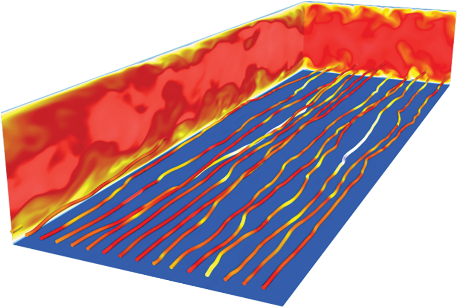
Figure 1: Turbulent channel flow (source: [1])

Consequently to these validations, the aim of the proposed CFD model is to predict the dispersion of particles in the atmosphere, for an area on the order of the hectometer, taking into account detailed geometries of the topography. However, correctly resolving the atmospheric boundary layer is not straight forward and its representation needs to be validated first. In article [2], a Schumann’s wall model was implemented and tested in 2D. It used the Streamline Upwind Petrov-Galerkin (SUPG) stabilization method implemented by Janssens [1] to stabilize the numerical oscillations. The results were encouraging but in 3D, spurious numerical fluctuations near the wall were observed. There are suspicions concerning the stabilization currently used in our finite element method. It appears as insufficient to damp the oscillations occurring with high Reynolds number flow. So, we intend to amend it using the techniques from the Variational Multiscale Method (VMS), which provides a combined framework for stabilization and turbulence modeling. In this article, the proposed solution is first described and then compared theoretically to the SUPG method. In the second part, a comparison is proposed on the Taylor-Green test case and the results are being analyzed.

2  Theory

In current work, the described methods are implicit. Thus, the system of equations is coupling the velocity and the pressure.

2.1 Navier-Stokes in FEM

The model that is being implemented is based on the incompressible two Navier-Stokes transport equations. These can be written following [1]:

∇⋅u=0

∂u∂t+(u⋅∇)u+u(∇⋅u)2+∇p−ν∇2u=0 (1)

The finite element formulation of the continuity and momentum equations can be achieved by multiplying these equations with weighting functions. The unknown variables can be interpolated between the discrete nodes by using shape functions and eventually, these equations can be integrated over the whole domain. The expressions can be simplified by choosing weighting functions equal to shape functions, which leads to a Galerkin formulation. After applying a θ-method to the time derivative and because the shape functions are non-zero only on their respective node and surrounding element, the integrals for all the elements can be replaced by a sum of the integral on each element. By solving this discrete system, the pressure and the velocity for the next timestep can be found:

∑e=1N⁡(1ΔtTe+θAe)(xen+1−xen)=−Aexen (2)

where θ is set to 1 for a forward Euler scheme or 0.5 for a Crank-Nicolson scheme. By default, it is set to 0.5 in [1]. The unknown xen for each element, grouped by nodal values, have following format for a 3D element with m + 1 nodes:

xen=[p0n⋯pmn(u0n)0⋯(u0n)m⋯(u2n)m] (3)

Matrices Ae and Te have the following structure:

Ae=[AppApuAupAuu]=[AppApu0Apu1Apu2Au0pAu0u0Au0u1Au0u2Au1pAu1u0Au1u1Au1u2Au2pAu2u0Au2u1Au2u2] (4)

2.2 SUPG Stabilization Method

By applying the SUPG stabilization method detailed in [3] to Eq. (1), each block of Ae can be formulated as follows:

App=∫Ωe⁡τPS∇NpT∇NpdΩe (5)

Apui=∫Ωe⁡((Np+τPSu~adv∇Np2)T(∇Nu)i+τPS(∇Np)iTu~adv∇Nu)dΩe (6)

Auip=∫Ωe⁡(Nu+τSUu~adv∇Nu)T∇NpdΩe (7)

Auiui=∫Ωe⁡(ν∇NuT∇Nu+(Nu+τSUu~adv∇Nu)Tu~adv∇Nu)dΩe+Auiuj (8)

Auiuj=∫Ωe⁡(τBU(∇Nu)i+12(u~adv)i(Nu+τSUu∇Nu))T(∇Nu)jdΩe (9)

Tpui=∫Ωe⁡τPS(∇Np)iTNudΩe (10)

Tuiui=∫Ωe⁡(Nu+τSUu~adv∇Nu)TNudΩe (11)

where u~adv is the advection velocity, obtained, in [1], by a Taylor expansion of the previous velocities. And where the stabilization terms, multiplied by their respective stabilization coefficients (τPS, SU, BU), are presented in [4]. These coefficients have to be chosen in such a manner that the numerical values are properly stabilized but not over-dissipated. This stabilization method was implemented by Janssens in [1] and successfully helped to solve oscillations for reasonable Reynolds simulation (e.g., the channel flow test case). Nevertheless, to be able to tackle the spurious numerical oscillations observed in [5], the idea is to use a generalized version of the SUPG stabilization method, called Variational Multiscale method (VMS), introduced by Hughes in [6]. The next section will present an implementation of the VMS algorithm proposed by Bazilevs [7].

2.3 Variational Multiscale Method (VMS)

The VMS applies the scale separation (coarse vs. fine) primarily and only approximate the fines scales. In these small scales, the stabilization terms appear “naturally”.

2.3.1 Structure

The proposed VMS method follows a predictor/multi-corrector structure, schematized in Fig. 2. This method has more parameters than the standard SUPG method, allowing it to better respond to numerical oscillations.

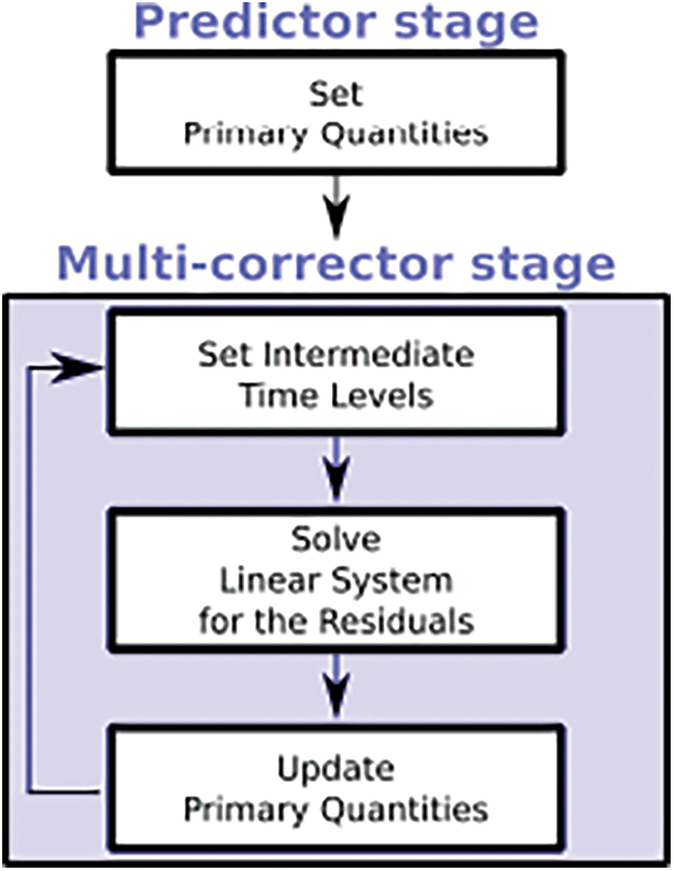
Figure 2: Predictor/Multi-corrector’s structure

2.3.2 Stages

Predictor stage

For each timestep, during the first stage, the predictor stage, the three variables (velocity u, derivative of the velocity u⋅ and pressure p) are set according to previous timestep.

Un+1,(0)=Un (12)

U˙n+1,(0)=γ−1γU˙n (13)

Pn+1,(0)=Pn (14)

γ (as well as αf and αm that are presented in this section) is a real-valued parameter defining the α-method. It is developed in [8,9].

Multi-corrector stage

Then, a number of iterations (l = 1, 2, …, lmax) is performed (typically between 2 and 4) to converge to steady values, or in other words, the residuals for, both, the continuity and momentum equations of Eq. (1) are minimized. To be more explicit, during these iterations, the following steps are performed:

1)   The first step is to set the intermediate time levels:

U˙n+αm,(l)=U˙n+αm(U˙n+1,(l−1)−U˙n) (15)

Un+αf,(l)=Un+αf(Un+1,(l−1)−Un) (16)

Pn+1,(l)=Pn+1,(l−1) (17)

αf and αm are intermediate time level parameters. They (as well as previously mentioned γ) are selected, taking accuracy and stability considerations into account. According to [9], obtaining second-order accuracy in time is possible if:

γ=12+αm−αf (18)

and the method is unconditionally stable if:

αm≥αf≥12 (19)

2)   These intermediate values are used to assemble the residuals of the continuity and momentum equations and solve the following linear system:

Au˙u˙ΔU˙n+1,(l)+Au˙pΔPn+1,(l)=−R(l)M (20)

Apu˙ΔU˙n+1,(l)+AppΔPn+1,(l)=−R(l)C (21)

that can be rearranged as below:

[Au˙u˙Au˙pApu˙App][ΔU˙n+1,(l)ΔPn+1,(l)]=[−R(l)M−R(l)C] (22)

3)   This will provide values for the derivative of the velocity and the pressure that can be updated in the last step of the multi-stage corrector:

U˙n+1,(l)=U˙n+1,(l−1)+ΔU˙n+1,(l) (23)

Un+1,(l)=Un+1,(l−1)+γΔtΔU˙n+1,(l) (24)

Pn+1,(l)=Pn+1,(l−1)+ΔPn+1,(l) (25)

In terms of computation, the second step of the multi-corrector stage, namely, assembling and solving the linear system, is the costliest.

2.3.3 VMS Assembly Matrix Ae

Below, compared to Eqs. (5)–(11), a slightly different assembly matrix Ae is provided:

Ae=[Au˙u˙Au˙pApu˙App] (26)

Indeed, in this case, the first block depends on the derivative of the velocity u⋅ and the last block on the pressure p. This structure was chosen to match the proposed implementation of [7] but it is equivalent to the one presented in the SUPG Section 2.2.

For each block, the expression is detailed hereafter:

Au˙iu˙i=∫Ωe⁡(αmNu˙TNu˙+αm(uτM∇Nu˙)TNu˙+αfγΔtNu˙Tu∇Nu˙+αfγΔt(∇Nu˙ν)T∇Nu˙+αfγΔt(u∇Nu˙τM)T(u∇Nu˙))dΩe (27)

Au˙iu˙j=∫Ωe⁡(αfγΔt(∇Nu˙)jTν(∇Nu˙)i+αfγΔt(∇Nu˙)iTτC(∇Nu˙)j)dΩe (28)

Au˙ip=∫Ωe−(∇Nu˙)iTNp+(uTτM(∇Nu˙)i)T∇NpdΩe (29)

Apu˙i=∫Ωe⁡(αfγΔtNpT(∇Nu˙)i+αfγΔt(∇Np)iTτMu∇Nu˙+αm(∇Np)iTτMNu˙)dΩe (30)

App=∫Ωe⁡(∇Np)TτM∇NpdΩe (31)

As previously described, the N[u˙,p] represent the shape functions; α[f,m] and γ the intermediate time level parameters; Δt the difference between timestep tn+1 and tn; u is the advection velocity (different of u~adv because computed during the simulation and not constructed from a Taylor serie); ν is the kinematic viscosity; and τ[C,M] are the stabilizing coefficients that still needs to be described thoroughly.

2.3.4 Defining the Stabilizing Coefficients

τM and τC are the stabilizing coefficients associated to the momentum and continuity equations. Below, their respective expressions:

τM=(4Δt2+uh⋅Guh+C1ν2G:G)−12 (32)

τC=(τMg⋅g)−1 (33)

where C1 is a positive constant, derived from an element-wise inverse estimate described in [10] and set to 1 in our work. And where three specific operations have to be introduced:

1.    The tensor product G:G=∑i,j=13⁡GijGij

2.    The tensor product uh⋅Guh=∑i,j=13⁡uihGij(ujh)T

3.    The tensor product g⋅g=∑i=13⁡gi(gi)T

where Gij=∑k=13⁡Jk,i−1(Jk,j−1)T is the element metric tensor, computed from the element shape function inverse Jacobian matrix J−1=(∂xi∂ξk)−1 . For the last item gi=∑j=13⁡(J−1)j,i .

2.4 SUPG vs. VMS Assembly Matrix Comparison

Now that both SUPG (2.2) and VMS (2.3) are described, it is convenient to show that, indeed, the VMS method can be considered as a generalized version of the older and more used SUPG method.

To ease the comprehension, the intermediate time level parameters are set to unity: αf = αm = γ = 1, and Δt is set equal to 1 making the value of u˙ and u equal.

For each block of the assembly matrices, the observation is given:

1.    PP block (Eqs. (5), (31)): Both equations are expressing the shape functions related to the pressure and can be considered equivalent, assuming τPS ≡ τM

2.    PUi block (Eqs. (6), (10), (30)): Both Ae and Te for SUPG are gathered into Ae in VMS. Besides, Eq. (6) is proportional to the two first terms of Eq. (30), while the third term in Eq. (30) is equivalent to Eq. (10).

Note that the second term of the SUPG formulation is written in skew symmetric form to improve its stability and accuracy properties.

3.   UiP block (Eqs. (7), (29)): After an integration by parts, the first term of Eq. (7) can be expressed as the first term of Eq. (29). The second terms are directly equivalent.

This also implies that, for setting the pressure to 0 on a boundary (i.e., at the outlet), nothing has to be done. It is the “do-nothing” boundary condition [11].

4.   UiUi block (Eqs. (8), (11), (27)): All the terms are identical.

5.   UiUj block (Eqs. (9), (28)): In the last block, there is a clear distinction between the SUPG and the VMS formulation. For the first term of Eq. (9), supposing τBU ≡ τC, it can be considered equivalent to the second term of Eq. (28). The second term of Eq. (9) is the skew-symmetric form in the SUPG matrix while the viscous tensor in VMS is treated differently.

3  Results

Now that the VMS theory that is implemented has been described, a few tests will be presented.

Note that, to reduce the computer cost, all tests are performed in 2D.

The first section is focused on the structure of the algorithm whereas the second, on the implementation.

3.1 VMS Structure: Poisson and Taylor-Green

The VMS structure described in Section 2.3.1 is a predictor/multi-corrector structure. To confirm the correctness of our implementation, it was first tested qualitatively, with classical equations that have analytical values.

The two chosen tests are the Poisson equation (with a uniform velocity boundary condition) for its simple implementation and the Taylor-Green equation for its periodical boundary conditions (Fig. 3).

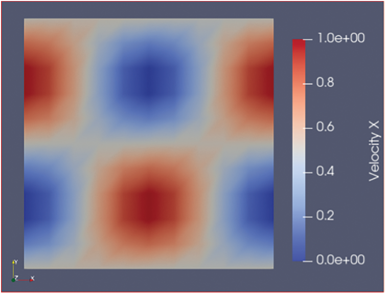
Figure 3: Taylor-Green test case

The objective of these tests was to ensure the output, with the new structure, would correlate with the one produced with a standard Navier-Stokes structure.

3.2 Tests for the VMS Implementation

Having acquired confidence in the structure, the next step was to test the algorithm’s implementation. The latter is more complicated because the only comparison that can be performed is to compare the assembly matrix Ae between the SUPG implementation and the VMS algorithm implementation, when both the viscosity ν and the stabilization coefficients τx are reduced to zero.

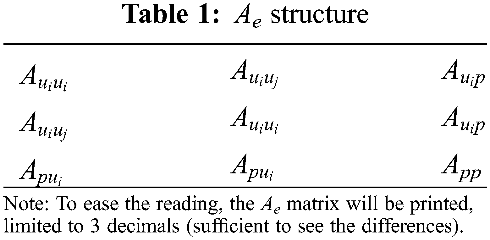
To better analyse how each equation described in Section 2.3.3 is influencing Ae, they are schemed with blocks in Table 1. Note that each block is actually a 3 × 3 matrix.

3.2.1 Results with ν = τx = 0

A simulation was performed, for an identical mesh, with both the SUPG implementation and the VMS implementation. Table 2 displays Ae for the SUPG implementation. This is the reference result.

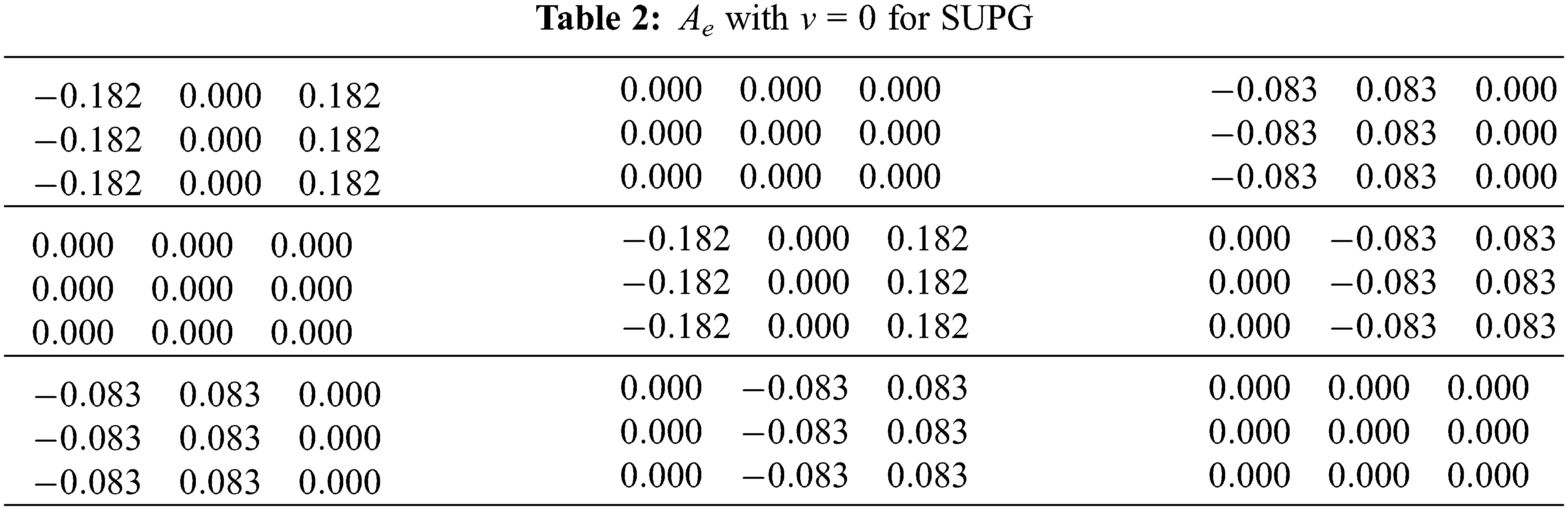
In Table 2, one can see the matrix is symmetrical, considering the blocks. Another observation is that Auiuj and App blocks are null value. Eventually, all blocks have a column structure (values varying only column-wise).

The next table (Table 3) proposes the VMS implementation (Eqs. (27)–(31)).

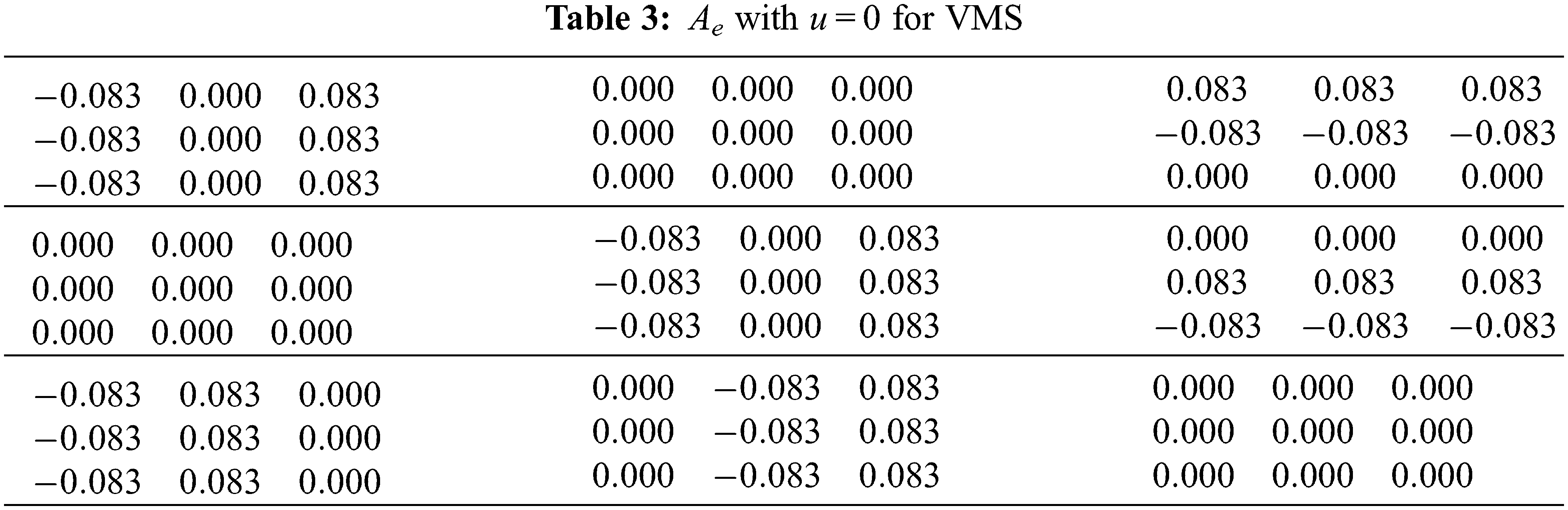
When analysing Table 3 for the similarities, the observation is that the null valued blocks are identical. For the differences, the first remark is that Ae is column-wise except for Auip that is row-wise and has the opposite sign, compared to SUPG values. Second, the Auiui values are not equal to SUPG ones.

After modifying Auip by transposing it and taking its opposite value, Table 3 becomes Table 4.

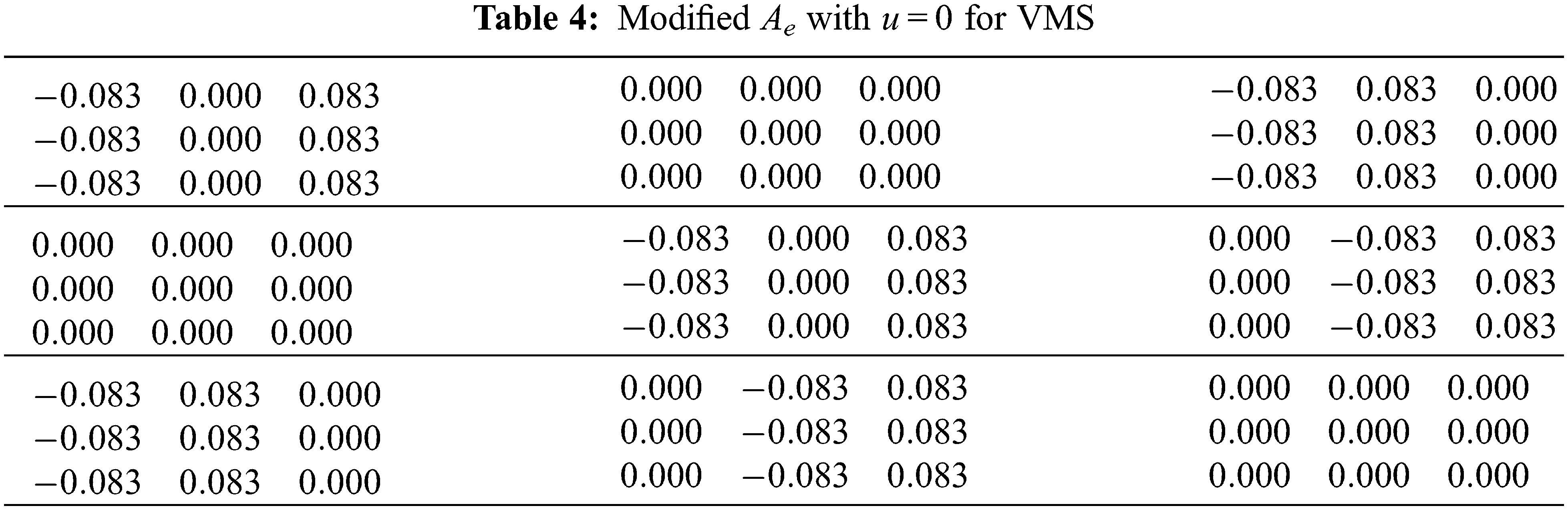
In the latter, the only difference resides in Auiui . This issue is still under investigation. When the issue will be solved, the next step will be to reactivate the stabilization coefficients and the viscosity to study their behavior.

4  Conclusion

In this article, after having acknowledged the purpose of the work and its context, the aim was to present the Variational Multiscale Method, to describe the chosen implementation, to demonstrate that it can be considered as a more general version of the SUPG method, and to present its similarities and differences with that method.

In the first part, the main objective of the work and its context were briefly recalled.

Then, in the second part, a theoretical explanation was provided for these two methods. Their respective assembly matrices were described and a comparison revealed their characteristics.

The third part was more focused on the results of the implementation. It was shown that the predictor/multi-corrector stages structure was properly implemented. It was also shown that the implementation of the algorithm itself is not yet correct although evolving in the right direction.

Eventually, when the VMS implementation will reflect perfectly the SUPG (for the non-viscous case), it will offer a robust foundation to explore the VMS capacities.

Acknowledgement: This study is promoted by the Royal Military Academy (RMA), in cotutelle with the Université de La Rochelle (ULR) and the von Karman Institute for Fluid Dynamics (VKI). The author is thankful to these three institutions to give him the opportunity to work on this subject.

Funding Statement: The authors received the funding of the Royal Higher Institute for Defence (MSP16-06).

Conflicts of Interest: The authors declare that they have no conflicts of interest to report regarding the present study.

References

1. Janssens, B. (2014). Numerical modeling and experimental investigation of fine particle coagulation and dispersion in dilute flows (Ph.D. Thesis). Universite de La Rochelle. [Google Scholar]
2. Nishio, Y., Janssens, B., van Beeck, J., Limam, K. (2019). CBRN dispersion modeling in the atmosphere. Review of the VKI Doctoral Research 2018–2019, pp. 85–93. Von Karmann Institute for Fluid Dynamics, Belgium. [Google Scholar]
3. Banyai, T., van Abeele, D., Deconinck, H. (2006). A fast fully-coupled solution algorithm for the unsteady incompressible Navier stokes equations. Conference on Modelling Fluid Flow (CMFF’06), pp. 91–98. Budapest, Hungary. [Google Scholar]
4. Braack, M., Burman, E., John, V., Lube, G. (2007). Stabilized finite element methods for the generalized oseen problem. Computer Methods in Applied Mechanics and Engineering, 196(4–6), 853–866. DOI 10.1016/j.cma.2006.07.011. [Google Scholar] [CrossRef]
5. Nishio, Y., Janssens, B., Limam, K., van Beeck, J. (2018). Multiphase flow modeling for CBRN applications. International Conference on Materials and Energy (ICOME’18), San Sebastian, Spain. [Google Scholar]
6. Hughes, T. J., Mazzei, L., Jansen, K. E. (2000). Large Eddy Simulation and the variational multiscale method. Computing and Visualization in Science, 3(1–2), 47–59. DOI 10.1007/s007910050051. [Google Scholar] [CrossRef]
7. Bazilevs, Y., Calo, V., Cottrell, J., Hughes, T. J., Reali, A. et al. (2007). Variational multiscale residual-based turbulence modeling for large eddy simulation of incompressible flows. Computer Methods in Applied Mechanics and Engineering, 197(1–4), 173–201. DOI 10.1016/j.cma.2007.07.016. [Google Scholar] [CrossRef]
8. Chung, J., Hulbert, G. M. (1993). A time integration algorithm for structural dynamics with improved numerical dissipation: The generalized-α method. Journal of Applied Mechanics, 60(2), 371–375. DOI 10.1115/1.2900803. [Google Scholar] [CrossRef]
9. Jansen, K. E., Whiting, C. H., Hulbert, G. M. (2000). A generalizedα method for integrating the filtered Navier–stokes equations with a stabilized finite element method. Computer Methods in Applied Mechanics and Engineering, 190(3), 305–319. DOI 10.1016/S0045-7825(00)00203-6. [Google Scholar] [CrossRef]
10. Johnson, C. (2012). Numerical solution of partial differential equations by the finite element method. In: Dover books on mathematics series, Courier Corporation. [Google Scholar]
11. Braack, M., Mucha, P. B. (2014). Directional do-nothing condition for the Navier-stokes equations. Journal of Computational Mathematics, 32(5), 507–521. DOI 10.4208/jcm.1405-m4347. [Google Scholar] [CrossRef]
Cite This Article
Copyright © 2023 The Author(s). Published by Tech Science Press.
This work is licensed under a Creative Commons Attribution 4.0 International License , which permits unrestricted use, distribution, and reproduction in any medium, provided the original work is properly cited.
Downloads
Citation Tools