
 Submit a Paper
 Propose a Special lssue
 Open Access
ARTICLE
Numerical Analysis of the Tunnel-Train-Air Interaction Problem in a Tunnel with a Double-Hat Oblique Hood
1 School of Mechanics and Engineering, Southwest Jiaotong University, Chengdu, 610031, China
2 State Key Laboratory of Traction Power, Southwest Jiaotong University, Chengdu, 610031, China
* Corresponding Author: Minglu Zhang. Email:
Fluid Dynamics & Materials Processing 2023, 19(2), 345-359. https://doi.org/10.32604/fdmp.2022.020233
Received 12 November 2021; Accepted 12 April 2022; Issue published 29 August 2022
 View Full Text
 Download PDF
Abstract
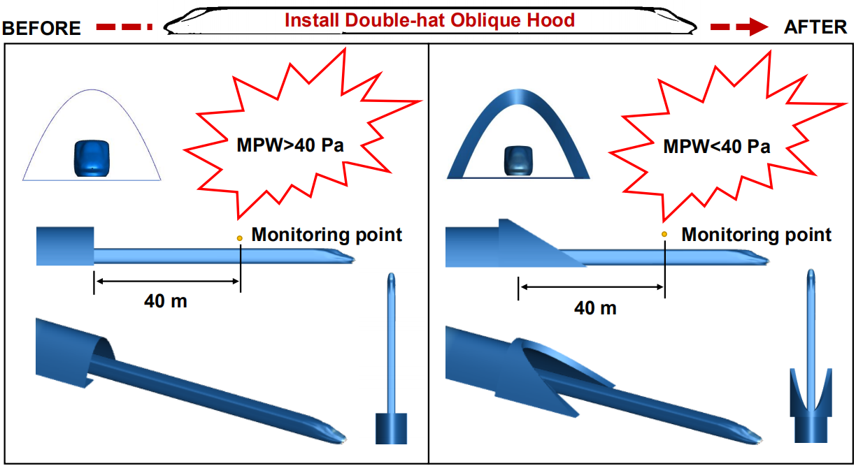
The tunnel-train-air interaction problem is investigated by using a numerical method able to provide relevant information about pressure fluctuations, aerodynamic drag characteristics and the “piston wind” effect. The method relies on a RNG k-ε two-equation turbulence model. It is shown that although reducing the oblique slope can alleviate the pressure gradient resulting from initial compression waves at the tunnel entrance, the pressure fluctuations in the tunnel are barely affected; however, a large reduction of micro-pressure wave amplitudes is found outside the tunnel. In comparison to the case where no tunnel hood is present, the amplitudes of micro-pressure waves at 40 m from the tunnel reach an acceptable range. The aerodynamic drag of the head and tail fluctuates greatly while that of the intermediate region undergoes only limited variations when the high-speed train passes through the double-hat oblique tunnel. It is shown that the effects of the oblique slope of the portal on the aerodynamic drag can almost be ignored while the train speed plays an important role.Graphic Abstract
Keywords
High-speed railways usually employ straight lines, large curve radii, and small slopes such that bridges and tunnels account for a large proportion of the total length of the railway line in regions with vast expanses and mountainous areas [1].
With the increasing speed of high-speed trains passing through tunnels, the aerodynamic performance of tunnels is attracting greater attention. Problems such as micro-pressure wave, wake flow, and piston wind induced by a passing train not only pose threats to safe and stable train operation but also reduce passenger comfort. In many countries, these problems are usually alleviated by optimizing the opening rate of tunnel hoods [2–4] and redesigning tunnel portals [5–7]. Studies have shown that some new tunnel portals can effectively reduce the pressure gradient. In particular, hat oblique tunnel portals have the most obvious effects in terms of alleviating the amplitudes of micro-pressure waves at the tunnel exit; hence, they are widely used in engineering practice, such as passenger dedicated lines [8]. Based on a railway passenger line project, Liu [9] presented a detailed analysis of the construction difficulties and the buffering effects of a combination of the hat oblique portal and tunnel hood at the entrance under actual working conditions. Zhang et al. [10] presented a 1:20 scale moving model to study the mitigation of micro-pressure waves by a combination of the hat oblique portal and top opening hood. Guo et al. [11] comprehensively studied the effect of several architectural parameters of the hat oblique portal on micro-pressure waves in tunnels.
All aforementioned studies suggest that appropriate settings of hat oblique portals at tunnel entrances can effectively alleviate the aerodynamic effects of tunnels. However, according to statistics on the construction of tunnel hoods at entrances, the mitigation effects on micro pressure waves gradually decrease as the length of the tunnel hood increases beyond a certain threshold. Furthermore, many commonly used measures (such as changing the streamline of the train head and setting hoods at tunnel entrances) have economic and commercial limitations [12]. In addition, the construction of tunnel hoods is restricted by insufficient terrain space, complicated operations, etc. Increasing the length of tunnel hoods at entrances poses a major challenge to the current construction methodology. Some studies have shown that setting up different portal forms and tunnel hoods at exits can significantly reduce micro-pressure wave amplitudes and noise [6,13]. To overcome the drawbacks of previous studies, this study proposes a novel tunnel model equipped with double-hat oblique portals and tunnel hoods to reduce the aerodynamic side effects and increase the feasibility of using tunnel hoods.
This study aims to establish a three-dimensional numerical model for investigating micro-pressure waves at the exits of tunnels and aerodynamic drag fluctuations when high-speed trains pass through a double-hat oblique tunnel. The results can provide guidelines for designing high-speed railway tunnels.
The passing of a high-speed train through a tunnel can be regarded as a transient problem. The air in the tunnel is squeezed between the train surface and the tunnel wall; hence, it can be treated as a compressible ideal gas. The airflow around the train is strongly disturbed; in general, the Reynolds number is greater than 106 and the flow field is in a turbulent state [14]. Therefore, this study employs the commonly used renormalization group (RNG) k-ε two-equation turbulence model to simulate the fluctuating process of the flow fields when trains pass through the tunnel. The governing equations are expressed as follows [15]:
Mass conservation equation:
Energy conservation equation:
Momentum equation in the x-direction:
Momentum equation in the y-direction:
Momentum equation in the z-direction:
Turbulent kinetic energy equation:
Turbulent dissipation equation:
At high Reynolds numbers, the turbulent viscosity (
where
2.2 Geometric Model and Boundary Conditions
Fig. 1 shows a simplified three-group model that is established on the basis of a certain type of Harmony train, where detailed structures such as pantographs, windshields, and bogies are ignored. The model has a length (L) of around 76 m, a width of 3.35 m, and a height of 3.50 m. It has been verified in [14] that the pressure calculated using the simplified train model is consistent with the pressure measured in the corresponding real train test in [16]. Therefore, these details are ignored in this study to improve computational efficiency. During the calculation, the boundary condition of the train surface is set as a non-slip wall. The layout of the three-dimensional model at the initial moment is shown in Fig. 2. When the train starts running, the head of the train is around 90 m from the tunnel entrance. The external atmosphere at both ports of the tunnel is simulated using a semi-cylinder with a radius of 190 m and a length of 250 m. Furthermore, the boundary condition of the semi-cylinder is set as the pressure outlet. The tunnel section, which has a length of around 400 m, is in the middle. Two hat oblique portals are installed in the two ports of the tunnel. The ports of the tunnel employ oblique slopes (the ratios of the height of the oblique section (H) to its length (D) are 1:1.00, 1:1.75, and 1:2.00, as shown in Fig. 3). The boundary conditions of the tunnel wall and the hat oblique portal are set to be a non-slip wall with a roughness of 0.5.
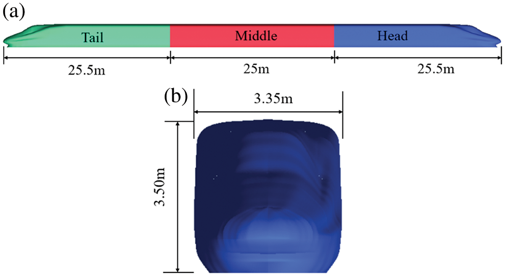
Figure 1: Geometric model of the train
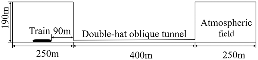
Figure 2: Overall layout of the geometric model
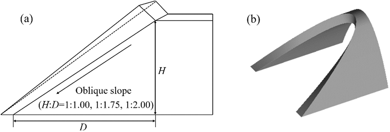
Figure 3: (a) Sketch and (b) 3D view of the hat oblique tunnel portal
2.3 Mesh Model and Solving Set
The train and tunnel models are divided using a structured hexahedral mesh in ANSYS ICEM. The slip grid is used for the train and the surrounding air to realize relative movement between the train and the ground. The static and moving areas exchange flow field information through the interface. To accurately simulate the evolution of the flow field around the body when the train passes through the tunnel, the thickness of the first layer of the train surface is set to 0.001 m; the boundary layer is expanded by 30 layers at a ratio of 1.05, and it then increases at a higher rate. The mesh size in the forward direction of the train changes from 0.1 m to 1 m while the mesh size of the body is around 0.15 m. The overall number of elements for the mesh model is around 8.8 million, of which the number of elements for the double-hat oblique portal is around 50,000. The mesh distributions of the train surfaces, tunnel, and boundary layer are shown in Figs. 4 and 5, respectively.
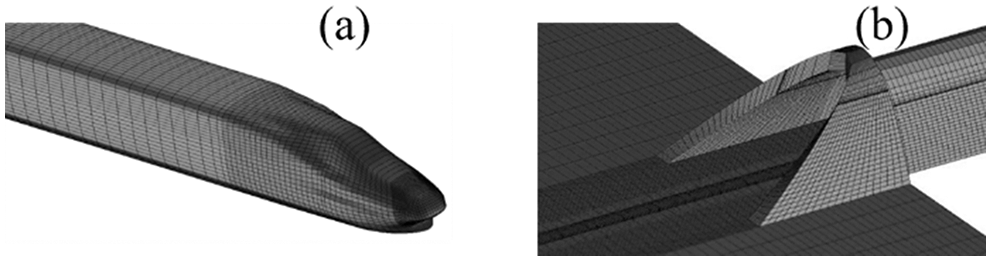
Figure 4: Meshes of (a) train and (b) tunnel
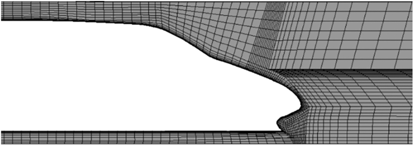
Figure 5: Mesh distribution at the boundary layer
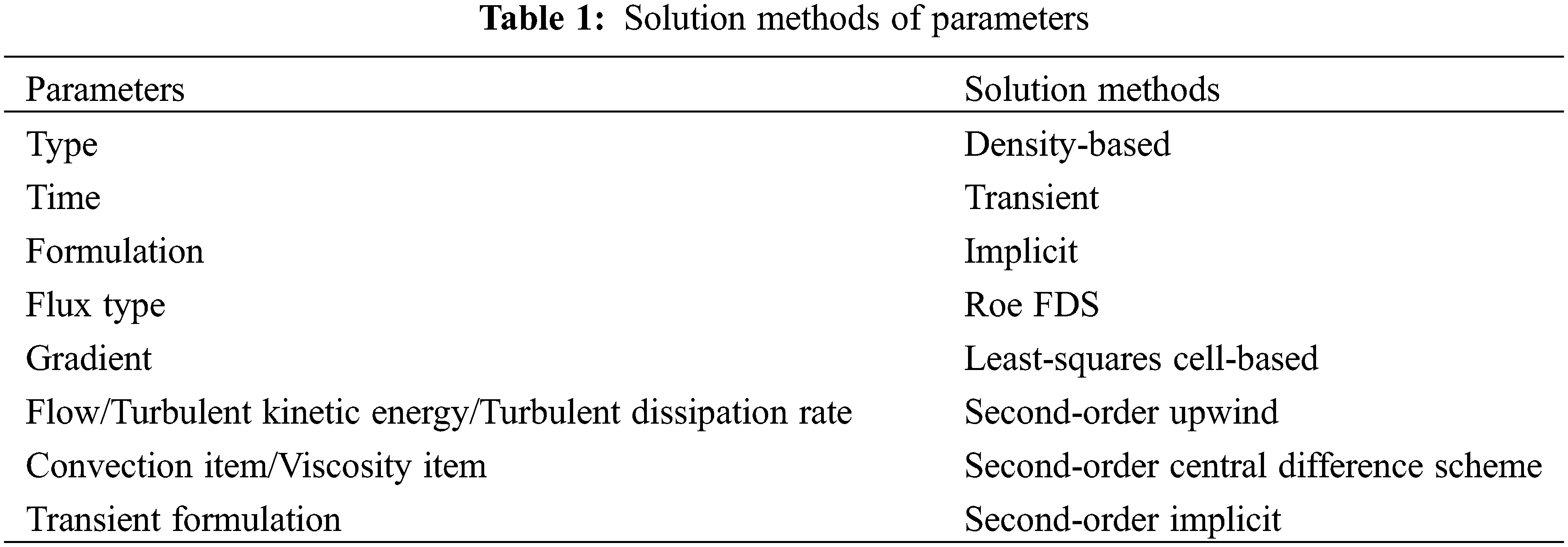
The meshed model is imported into ANSYS FLUENT CFD for calculation. The continuity and momentum equations are solved using a finite volume method [17]. Furthermore, a couple algorithm is used to solve discrete equations. The solution methods of the parameters are summarized in Table 1 [15]. The time step of the calculation is set to 1 × 10⁻³ s with 20 iterations in each time step, and the residual limit is 10−3. Deng et al. pointed out that the results calculated by using this time step are consistent with the results obtained by Schober et al. using a 1:15 scale train model [14,18]. The computing time is around 7.5 s.
The aerodynamic drag coefficient (
where
2.5.1 Analysis of Mesh Sensitivity
Two meshes with the same meshing strategy but different densities are constructed for mesh-independent analysis. The number of elements in the coarse mesh, which is the mesh model used in this study, is around 8.8 million. The fine mesh further refines the key areas, such as the train surface and the boundary layer; it contains more than 11.0 million elements.
As shown in Fig. 6, the results of the micro-pressure waves at the exit predicted by the coarse and fine meshes are consistent in terms of amplitude and trend. Specifically, the micro-pressure wave amplitudes calculated using the coarse and fine meshes are 0.0062 and 0.0061, respectively. The error is smaller than 2%. Thus, the mesh model used in this study can be employed for the following calculations.
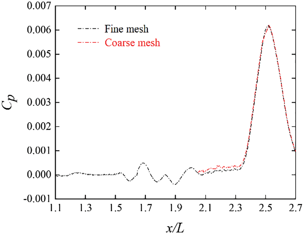
Figure 6: Comparisons of micro-pressure waves at the exit
2.5.2 Analysis of Mesh Sensitivity
Compared with the model used in [14], where the grid number is around 5.5 million, this study encrypts the flow field around the train to ensure high accuracy. As can be seen from [20], the change rate of the aerodynamic load in a time interval of 0.035 s can be used as an indicator of the degree of the impact of the aerodynamic load on the carriage. The maximum change rate of the aerodynamic load occurs when the corresponding carriage enters the tunnel. Table 2 summarizes the comparison of the maximum lift change rate (
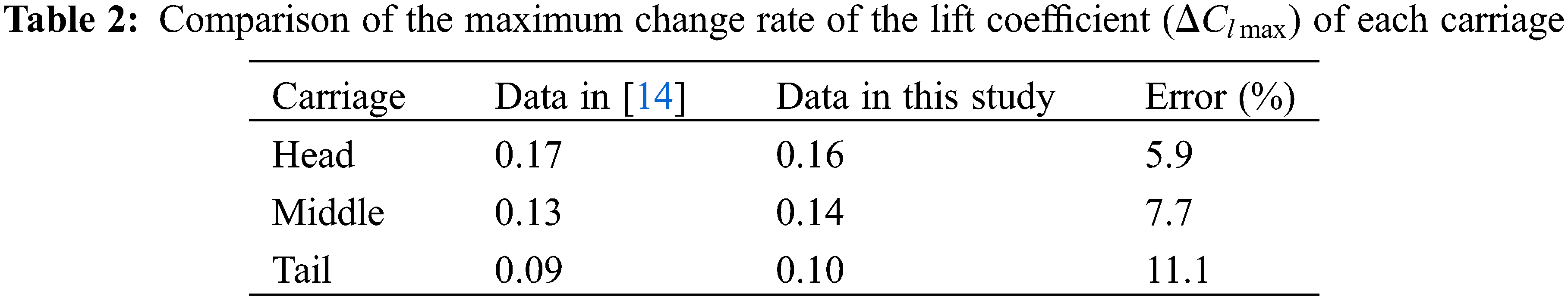
As can be seen from Table 2, the maximum lift change rate in this study is close to the data in [14] and the error is within an acceptable range. Thus, the numerical model used in this study can fulfill the calculation requirements and the numerical method is accurate.
Most of the compressed air flows forward together under the impetus of trains that pass through the tunnel at high speed [21]. This phenomenon is called the train piston effect, and the airflow is called the piston wind [22]. This is one of the factors that must be considered in tunnel ventilation design. Therefore, the velocity contour of the train passing through the tunnel at a speed of 350 km/h is selected to investigate the formation and fluctuation of the piston wind in the double-hat oblique tunnel, as shown in Fig. 7.
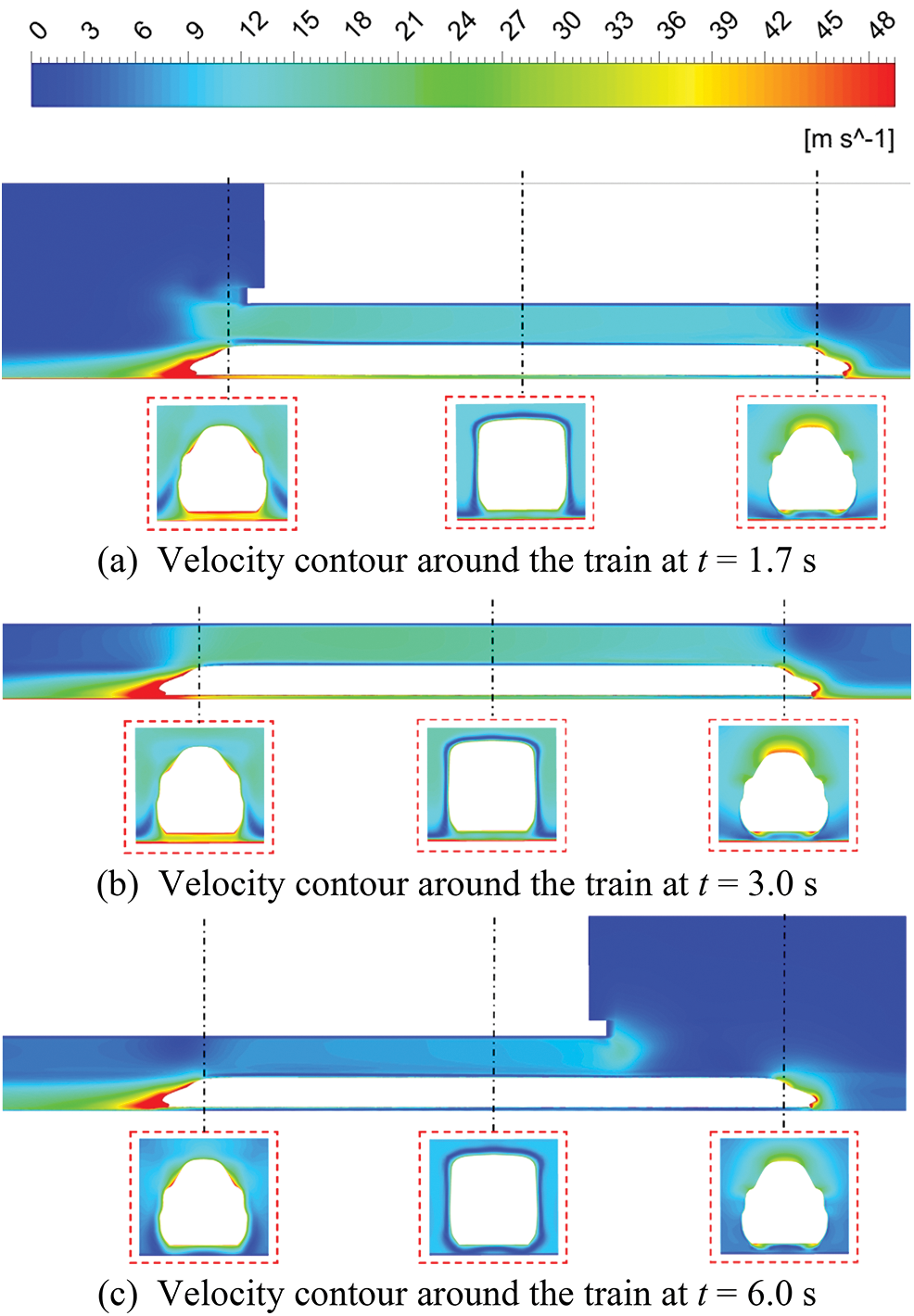
Figure 7: Velocity contour around the train at three moments
As can be seen from Fig. 7a, when the train enters the tunnel, the airflow in front of the train is hindered by the train head, and the incoming flow is stagnant at the train nose. Then, the flow velocity is reduced significantly. After flowing through the train head, the airflow around the train body gradually increases and then sprays at the tunnel entrance with a flow velocity of around 15 m/s. However, a strong wake flow is formed owing to the negative pressure at the rear of the train. As can be seen from Fig. 7b, when the train is running in the tunnel, owing to the boundary layer on the train surface, the airflow in the tunnel will advance with the train, and the airflow velocity first increases and then decreases. However, the fluctuation of the wake intensity is not obvious. As can be seen from Fig. 7c, when the train exits the tunnel, the flow field distribution at the head of the train is the same as that of the open line, which implies that the flow velocity is in a semicircular shape at the train head and radiates to the surroundings, while the wake flow still exists and the intensity does not change significantly.
3.2 Influence of Oblique Slope
Fig. 8 shows a comparison of the pressure and initial compression wave fluctuations at a distance of 30 m from the tunnel entrance when the train passes through the tunnel at a speed of 300 km/h under different oblique slopes. As can be seen from Fig. 8, owing to the long nose of the train head, the air in the tunnel is disturbed before the train enters the tunnel. At around point a, the air in front of the train is squeezed to form a compression wave when the high-speed train arrives at the tunnel entrance. At around point a, the compression wave reaches the monitoring point, causing the pressure to increase rapidly until the train head completely enters the tunnel, and it then reaches the first peak (point c). When the train head reaches the monitoring point, the pressure will increase again owing to the high pressure at the nose of the train head. At around point d, the pressure coefficient reaches its maximum value of around 0.42. The compression wave represented by the “a-b-c-d” segment in Fig. 8 is called an initial compression wave. When the train head passes the monitoring point, the pressure of the monitoring point starts to decline sharply owing to the cross-flow around the train body. Then, the expansion wave behind the train tail propagates to this point when the train is fully driven into the tunnel, which further reduces the pressure at the monitoring point, and it reaches the maximum negative pressure coefficient, which is around-0.51. Owing to the wake flow, the pressure at the monitoring point rapidly increases to 0 after the train passes the monitoring point. Then, the pressure at this point tends to be stable for some time. However, it will continue to fluctuate owing to the propagation and overlap of the compression and expansion waves.
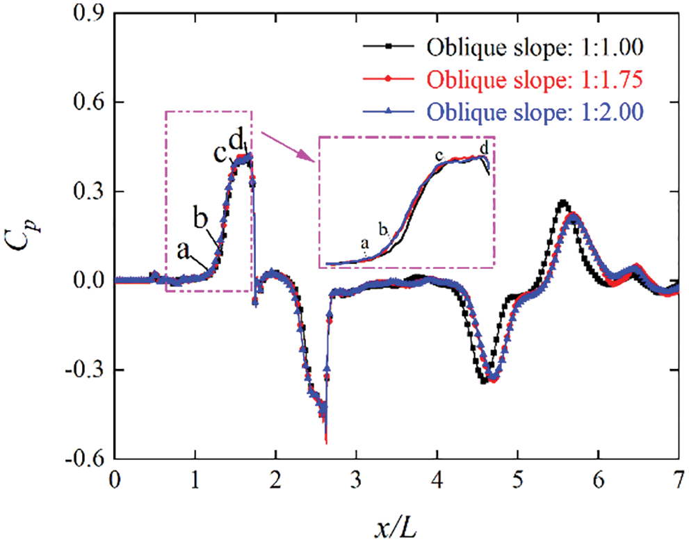
Figure 8: Pressure fluctuations at 30 m from the tunnel entrance
Further, As can also be seen from Fig. 8, when the high-speed train passes through the tunnel at three oblique slopes, they do not have significant effects on the trend and amplitude of the pressure in the tunnel. However, the initial compression wave at the monitoring point is divided into two rising stages of “ac” and “cd” under the three oblique slopes of the tunnel portal, and the amplitude of the initial compression wave (point d) is nearly the same. In particular, it should be noted that the time to reach the maximum value increases as the oblique slope decreases. Moreover, the first peak (point c) of the initial compression wave determines the amplitude of the micro-pressure wave at the tunnel exit.
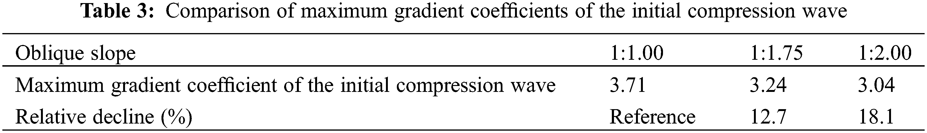
The comparison of the gradient amplitude of the initial compression wave at a distance of 30 m from the entrance is shown in Table 3. As can be seen from Table 3, when the oblique slope is 1:1.00, the gradient coefficient of the initial compression wave is the largest, i.e., around 3.71. When the oblique slope is 1:1.75, it is around 3.24. When the oblique slope is 1:2.00, it is the smallest, i.e., around 3.04, and the maximum drop is around 18.1%. Therefore, it can be concluded that the smaller the oblique slope of the portal, the better the relief effect on the transient pressure gradient.
3.3 Influence of Oblique Slope and Train Speed on the Micro-Pressure Wave
The micro-pressure wave is a typical infrasonic wave phenomenon in the aerodynamic effects of high-speed railway tunnels, which is characterized by low frequencies and long wavelengths [4,23].
Fig. 9 shows the fluctuations of the micro-pressure wave at the monitoring point around 40 m outside the tunnel exit when a high-speed train passes through the double-hat oblique tunnel. Table 4 summarizes the comparison of the amplitude of the micro-pressure wave at this monitoring point. As can be seen from Fig. 9 and Table 4, when the oblique slopes of the portal are 1:1.00, 1:1.75, and 1:2.00, the maximum coefficients of the micro-pressure waves outside the tunnel exit are 0.0092, 0.0086, and 0.0083, respectively, with a corresponding decrease of 6.5% and 9.8%. Therefore, reducing the oblique slope can effectively alleviate the amplitude of the micro-pressure wave.
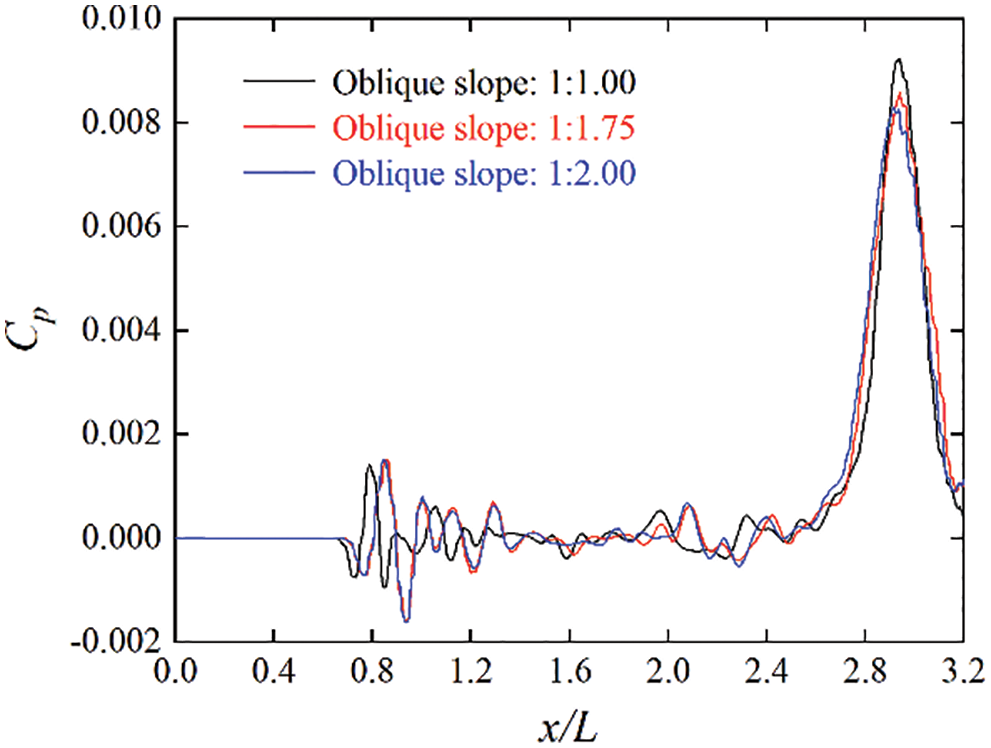
Figure 9: Micro-pressure wave fluctuations at around 40 m from the tunnel exit under three oblique slopes
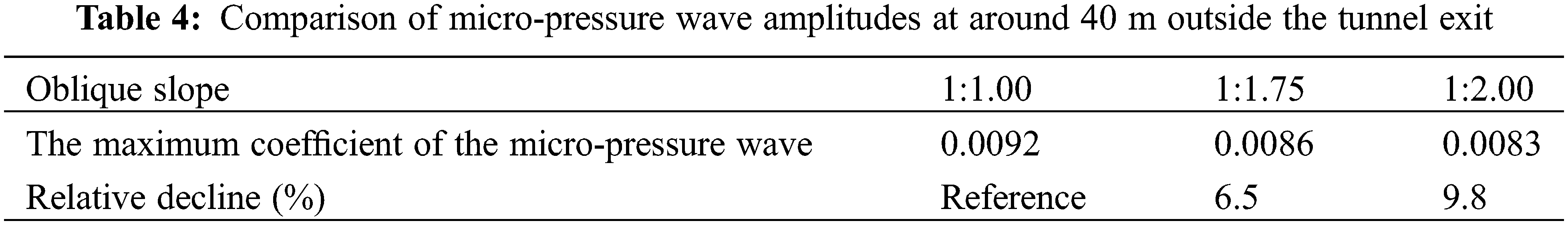
Fig. 10 shows a comparison of the micro-pressure wave fluctuations at the monitoring point when the train passes through the tunnel at two speeds. As can be seen from Fig. 9, when the train speed is 350 km/h, the maximum coefficient of the micro-pressure wave at this monitoring point is 0.0143, which is 35.7% higher than that when the train speed is 300 km/h. Thus, the train speed is an important factor affecting the micro-pressure amplitude.
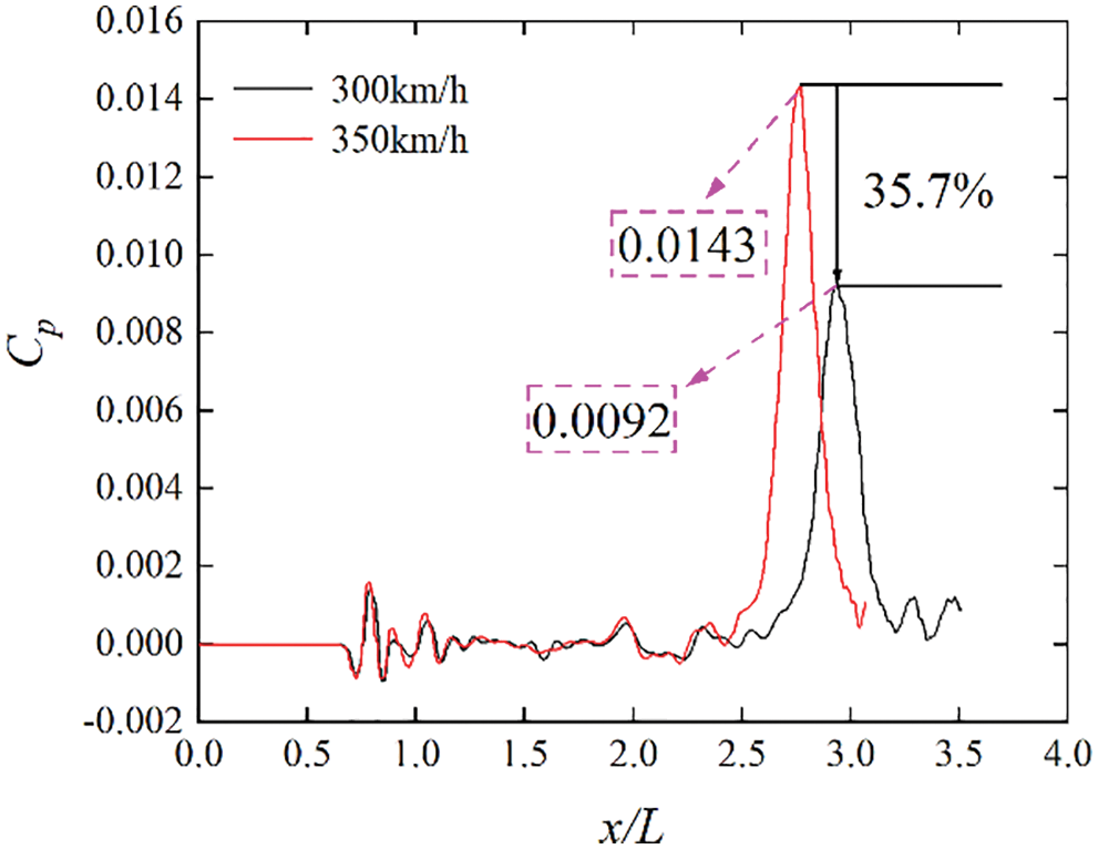
Figure 10: Micro-pressure wave fluctuations at around 40 m from the tunnel exit at two speeds
In [24], the micro-pressure wave coefficient reaches 0.0122 at 40 m outside the tunnel exit when a high-speed train passes through a tunnel without hoods under the same conditions. However, based on experience, the acceptable coefficient of the micro-pressure wave is around 0.0047–0.0094. Obviously, the mitigation effect of the micro-pressure wave can fulfill the requirements after the double-hat oblique tunnel portal is installed in the two ports of the tunnel in this study.
3.4 Fluctuations of Aerodynamic Drag
The flow field on the train surface undergoes alternating positive and negative fluctuations owing to the repeated action of the pressure when the high-speed train is running in the tunnel, which leads to complex fluctuations in the aerodynamic drag [25,26]. The aerodynamic drag can increase the energy consumption of the train and is difficult to measure. Thus, it is useful to analyze the trend of the aerodynamic drag. Moreover, it is important to discuss the influence of the train speed and the oblique slope of the tunnel portal on the aerodynamic drag (by considering the drag of the train head as an example).
Fig. 11 shows the fluctuation of the aerodynamic drag when the entire train passes through the tunnel with an oblique slope of 1:1.00 at a speed of 350 km/h. As can be seen from Fig. 11, when the train enters the tunnel, the drag increases sharply. Furthermore, the drag begins to decrease until the train completely enters the tunnel. The negative drag of the train appears when the train tail starts to pass through the tunnel midpoint, and it drops to the first valley value at t = 3.20 s. When the train leaves the tunnel, the maximum negative drag appears. Then, the train drag returns to the same value as that of the open line. Fig. 12 shows the pressure contour of the tunnel ground at t = 3.20 s. It can be clearly seen that the pressure behind the train tail is greater than that in front of the train head. The differential pressure between the tail and the head exerts a force on the train body that is in the same direction as the motion, which results in a negative aerodynamic drag.
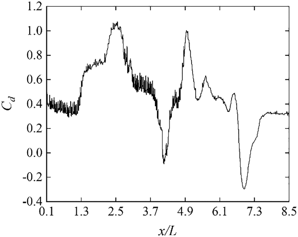
Figure 11: Drag fluctuation of the entire train
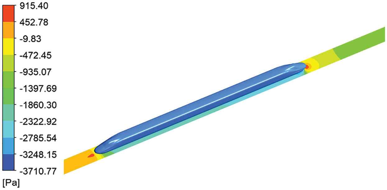
Figure 12: Pressure contour of the tunnel ground at t = 3.20 s
Fig. 13 shows the drag fluctuations of each carriage at a speed of 350 km/h. As can be seen from Fig. 13, the drag of the head and tail fluctuates severely during operation, while the fluctuation of the middle is relatively smooth. The head drag can also be understood to increase rapidly at the moment of entering the tunnel. Then, when the train head enters the tunnel completely, the drag increases gradually until the train tail begins to enter the tunnel, and the drag of the train head reaches its maximum value. At the same time, when the train tail starts to enter the tunnel, the drag of the train tail increases sharply. Furthermore, the drag of the train head begins to appear with a negative value when the train tail enters the tunnel completely. This can be interpreted as the transmission of the expansion wave from the front of the train to the rear of the train at this moment, and the strong negative pressure forms a “traction” in front of the train in the same direction as the motion. The drag of the train tail reaches its maximum value after passing through the midpoint of the tunnel and then begins to decrease. When the train tail exits the tunnel, the drag reaches its maximum negative value. This can be explained as follows. After multiple reflections, the compression waveforms a large resultant force at the rear of the train in the same direction as the movement. When the train passes through the tunnel, the drag of the intermediate train is always positive; the minimum value appears after the train passes through the midpoint of the tunnel, and the maximum value appears when the train reaches the tunnel exit. Fig. 14 shows the fluctuations of the train head drag at three speeds. As can be seen from Fig. 14, the higher the train speed, the more obvious the drag of the train head fluctuations and the farther back is the appearance of the maximum negative drag. Moreover, the maximum positive drag will appear when the train tail starts to enter the tunnel at three speeds. A comparison of the average drags of each carriage when the train passes through the tunnel under three oblique slopes is shown in Fig. 15. As can be seen from Fig. 15, the change in oblique slopes does not have significant effects on the aerodynamic drag of each carriage.
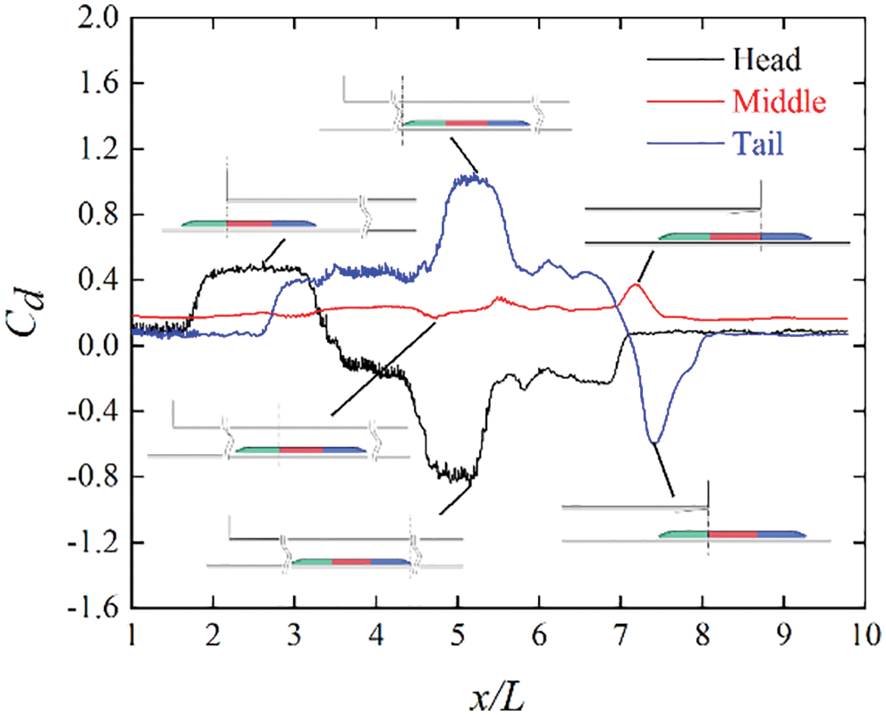
Figure 13: Drag fluctuations of each carriage
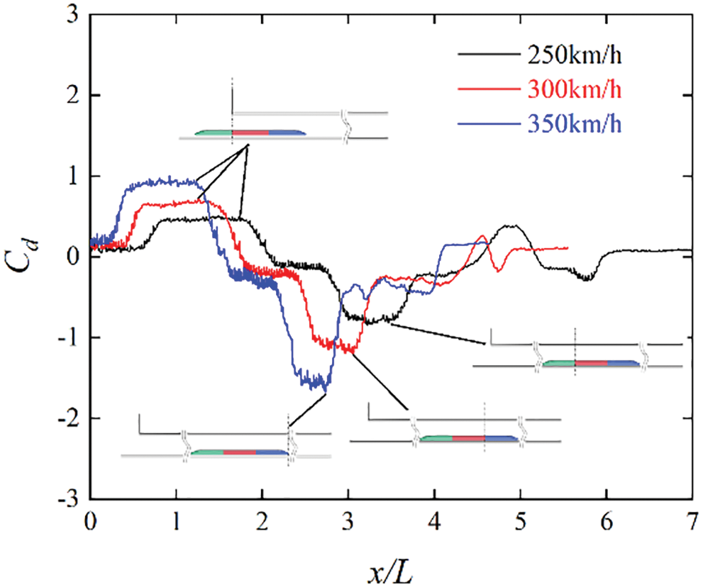
Figure 14: Drag fluctuations of the train head at three speeds
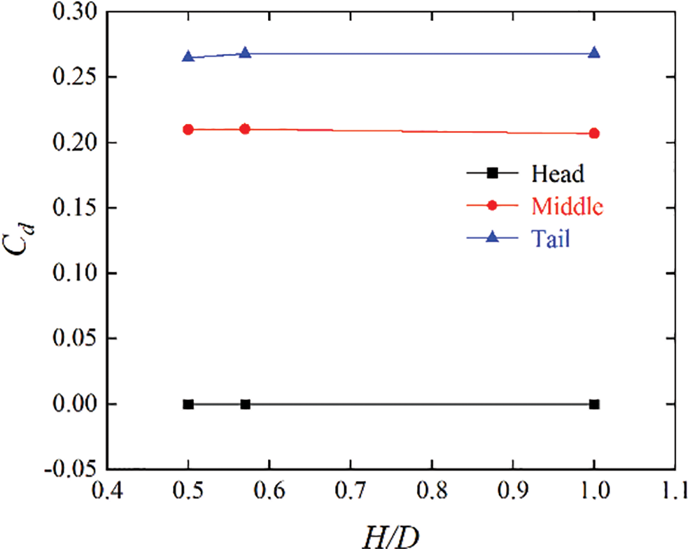
Figure 15: Average drag of each carriage at three oblique slopes
This study investigated the pressure fluctuations and aerodynamic drag characteristics of a high-speed train passing through a double-hat oblique tunnel using the Reynolds method and the RNG k-ε turbulence model. The following conclusions can be drawn on the basis of the established numerical model:
(1)The fluctuation of the piston wind induced by a passing train is complex and strong, while the wake flow always exists and the intensity change is not obvious.
(2)The reduction of the oblique slope has a significant mitigation effect on the gradient of the initial compression waves when a train passes through a tunnel, and the maximum decrease is around 18.1%.
(3)Compared with tunnels without hoods, the amplitude of the micro-pressure wave at 40 m from the tunnel exit is within an acceptable range when the double-hat oblique portal is set at the tunnel ports. The smaller the oblique slope, the more significant is the mitigation effect on the micro pressure wave outside the tunnel exit.
(4)The drag of the train head and tail fluctuates severely when the train passes through the tunnel, while the fluctuation of the intermediate train is gentle. The decrease in the oblique slope of the portal does not have significant effects on the train drag. However, the aerodynamic drag increases with the train speed.
Acknowledgement: The authors thank TopEdit (https://www.topeditsci.com) for its linguistic assistance during the preparation of this manuscript.
Funding Statement: This research was supported by the National Natural Science Foundation of China, China Grant (11972028), under the project “Analysis of Unsteady Aerodynamic Characteristics of High-Speed Train”.
Conflicts of Interest: The authors declare that we have no conflicts of interest to report regarding the present study.
References
1. Wang, K., Lü, K. (2016). Dynamic evaluation index system for spatial alignment of high-speed railway. Journal of Southwest Jiaotong University, 2(51), 227–235. [Google Scholar]
2. Takahashi, K., Honda, A., Yamagiwa, I., Nozawa, K., Doi, T. et al. (2016). Reduction of a micro-pressure wave by installing porous buffering plates in a branched outlet tunnel of a high-speed railway. Journal of Japan Society of Civil Engineers Ser A1, 72(1), 41–46. [Google Scholar]
3. Honda, A., Takahashi, K., Nozawa, K., Doi, T., Ogawa, T. (2015). Proposal of a porous hood for a high-speed railway tunnel based on an evaluation of a micro-pressure wave. Journal of Japan Society of Civil Engineers Ser A1, 71(3), 327–340. [Google Scholar]
4. Miyachi, T., Fukuda, T. (2021). Model experiments on area optimization of multiple openings of tunnel hoods to reduce micro-pressure waves. Tunneling and Underground Space Technology, 15(9), 103996. DOI 10.1016/j.tust.2021.103996. [Google Scholar] [CrossRef]
5. Winslow, A., Howe, M. S. (2005). Stepwise approximation of an optimally flared tunnel portal. Journal of Sound & Vibration, 280(3–5), 983–995. DOI 10.1016/j.jsv.2004.01.039. [Google Scholar] [CrossRef]
6. Gerbig, C., Degen, K. G. (2012). Acoustic assessment of micro-pressure wave emissions from high-speed railway tunnels. Notes on Numerical Fluid Mechanics & Multidisciplinary Design, 118(9), 389–396. DOI 10.1007/978-4-431-53927-8. [Google Scholar] [CrossRef]
7. Zhang, L., Kerstin, T., Norbert, S., Liu, H. (2018). Influence of the geometry of equal-transect oblique tunnel portal on compression wave and micro-pressure wave generated by high-speed trains entering tunnels. Journal of Wind Engineering and Industrial Aerodynamics, 178(10), 1–17. DOI 10.1016/j.jweia.2018.05.003. [Google Scholar] [CrossRef]
8. Luo, J. J., Wang, M. S., Gao, B., Wang, Y. X. (2007). Study on the compression wave induced by a high-speed train entering into a tunnel with hood (I). Acta Aerodynamica Sinica, 25(4), 488–494. [Google Scholar]
9. Liu, X. Q. (2008). Design and construction of buffer structure of large section loess tunnel portal. Journal of Railway Engineering Society, 25(7), 69–73. [Google Scholar]
10. Zhang, L., Yang, M. Z., Liang, X. F. (2017). Oblique tunnel portal effects on train and tunnel aerodynamics based on moving model tests. Journal of Wind Engineering and Industrial Aerodynamics, 167(21), 128–139. DOI 10.1016/j.jweia.2017.04.018. [Google Scholar] [CrossRef]
11. Guo, Z., Liu, T., Li, W., Xia, Y. (2021). Parameter study and optimization design of a hat oblique tunnel portal. Proceedings of the Institution of Mechanical Engineers, Part F: Journal of Rail and Rapid Transit, 1(1), 1–13. [Google Scholar]
12. Fukuda, T., Nakamura, S., Miyachi, T., Saito, S., Kimura, N. et al. (2018). Countermeasure for reducing micro-pressure waves by spreading ballast on the slab-track in the tunnel. Quarterly Report of Railway Technical Research Institute, 59(2), 121–127. DOI 10.2219/rtriqr.59.2_121. [Google Scholar] [CrossRef]
13. Hyo, G., Pan, K., G., C., Jio, H. Y. (2014). A study on the characteristics for aerodynamics at high speed in railway tunnels focused on the micro-pressure wave. Journal of Korean Tunnelling & Underground Space Association, 16(2), 249–260. DOI 10.9711/KTAJ.2014.16.2.249. [Google Scholar] [CrossRef]
14. Deng, E., Yang, W. C., Yin, R. S. (2019). Study on transient aerodynamic performance of high-speed trains when entering into tunnel under crosswinds. Journal of Hunan University (Natural Science Edition), 46(9), 69–78. [Google Scholar]
15. Zhao, J., Li, R. X., Liu, J. (2010). Numerical simulation of aerodynamic forces of high-speed trains passing each other at the same speed through a tunnel. Journal of the China Railway Society, 4(32), 27–32. [Google Scholar]
16. Liu, F., Yao, S., Liu, T. H. (2016). Analysis on aerodynamic pressure of tunnel wall of high-speed railway by full-scale train test. Journal of Zhejiang University (Engineering Science), 50(10), 2018–2024. [Google Scholar]
17. Deeb, R.J. (2021). Experimental and numerical investigation of the effect of angle of attack on air flow characteristics around drop-shaped tube. Physics of Fluids, 33(6), 065110. DOI 10.1063/5.0053040. [Google Scholar] [CrossRef]
18. Schober, M., Weise, M., Orellano, A., Deeg, P., Wetzel, W. (2010). Wind tunnel investigation of an ICE 3 end car on three standard ground scenarios. Journal of Wind Engineering and Industrial Aerodynamics, 98(6), 345–352. DOI 10.1016/j.jweia.2009.12.004. [Google Scholar] [CrossRef]
19. Suzuki, M., Tanemoto, K., Maeda, T. (2001). Aerodynamic characteristics of train/vehicles under cross winds. Journal of Wind Engineering & Industrial Aerodynamics, 91(1), 209–218. DOI 10.1016/S0167-6105(02)00346-X. [Google Scholar] [CrossRef]
20. Yang, W. C., Deng, E., Lei, M. F. (2019). Transient aerodynamic performance of high-speed trains when passing through two wind proof facilities under crosswinds: A comparative study. Engineering Structures, 188(2), 729–744. DOI 10.1016/j.engstruct.2019.03.070. [Google Scholar] [CrossRef]
21. Matsudaira, H., Sakakura, Y., Tanaka, Y., Nakada, T., Hamada, A. (1976). Dynamic characteristics of train wind in a tunnel: Part 1–Basic experiments in a model tunnel with a single line. Transactions of the Society of Heating, Air-Conditioning and Sanitary Engineers of Japan, 1(1), 67–73. [Google Scholar]
22. Yan, S. L., Ye, L., Yang, Q. (2020). Study on piston effect of Badaling tunnel and underground station of Beijing-Zhangjiakou high-speed railway. Railway Standard Design, 64(1), 75–80. [Google Scholar]
23. Kim, T. H., Dong, H. K., Rohit, I. S., Kim, H. D. (2019). Effect of the entry speed of high-speed train on tunnel micro-pressure wave. Journal of the Korean Society for Urban Railway, 7(2), 317–324. DOI 10.24284/JKOSUR.2019.6.7.2.317. [Google Scholar] [CrossRef]
24. Wang, C. (2014). Study on aerodynamic effect of high-speed train passing the short tunnel and tunnel group (Master Thesis). Dalian Jiaotong University, China. [Google Scholar]
25. Choi, J. K., Kim, K. H. (2014). Effects of nose shape and tunnel cross-sectional area on aerodynamic drag of train traveling in tunnels. Tunnelling and Underground Space Technology Incorporating Trenchless Technology Research, 41(3), 62–73. DOI 10.1016/j.tust.2013.11.012. [Google Scholar] [CrossRef]
26. Li, T., Dai, Z. Y., Yu, M. G., Zhang, W. H. (2021). Numerical investigation on the aerodynamic resistances of double-unit trains with different gap lengths. Engineering Applications of Computational Fluid Mechanics, 15(1), 549–560. DOI 10.1080/19942060.2021.1895321. [Google Scholar] [CrossRef]
Cite This Article
 Copyright © 2023 The Author(s). Published by Tech Science Press.
This work is licensed under a Creative Commons Attribution 4.0 International License , which permits unrestricted use, distribution, and reproduction in any medium, provided the original work is properly cited.
 Downloads
 Citation Tools