Fluid Dynamics & Materials Processing

DOI: 10.32604/fdmp.2022.019851

ARTICLE

Optimization of the Cooling System of Electric Vehicle Batteries

A. Heri Iswanto1,*, Iwan Harsono2, Alim Al Ayub Ahmed3, Sergushina Elena Sergeevna4, Stepan Krasnikov5, Rustem Zalilov6, John William Grimaldo Guerrero7, Liliya N. Latipova8 and Safa Kareem Hachim9

1Public Health Department, Faculty of Health Science, University of Pembangunan Nasional Veteran Jakarta, Jakarta, 16426, Indonesia
2Universitas Mataram, West Nusa Tenggara, 83116, Indonesia
3School of Accounting, Jiujiang University, Jiujiang, 330300, China
4National Research Ogarev Mordovia State University, Saransk, 430005, Russia
5Russian Technological University, Moscow, 119454, Russian
6Nosov Magnitogorsk State Technical University, Magnitogorsk, 455000, Russian
7Departamento de Energía, Universidad de la Costa, Barranquilla, 080002, Colombia
8Kazan Federal University, Kazan, 628400, Russia
9College of Technical Engineering, The Islamic University, Najaf, 54001, Iraq
*Corresponding Author: A. Heri Iswanto. Email: h.iswanto@upnvj.ac.id
Received: 20 October 2021; Accepted: 29 December 2021

1  Introduction

Conventional heat exchangers have several basic components. One of these components is a disk or plate that receives heat from a source such as a computer processor. The second component is a set of metal blades that help keep excess heat away from the plate or disc [1]. The last part, and in fact the most vital part of the coolers, is a fan that works by eliminating and dissipating heat around the metal blades and expelling the heat (Like the process you see behind the case of a home computer) [2–5]. This process has been a major component of these devices for almost half a century and has not changed. According to many researchers, this process has many inefficiencies, but the most important negative and dark point of this old procedure is that only 5% of the cooling fan energy in these systems is spent on cooling [6]. Many solutions have been proposed for this weakness, for example, they have increased the fan speed, but this solution is not suitable at all in terms of increasing the noise [7]. By increasing the speed of the cooling fans, we only increase the noise pollution, and our computers and other devices cause us more annoyance. In the new design, all these problems seem to be gone. Here, the fan and heat curtains become a component that sits on top of the disc and plate, and there is a thin layer of air between them. In this new and efficient design, fans and heat exchangers have a higher kinetic velocity, although this increase in velocity does not increase the noise, and this in addition to the loss of more heat and heat, also much less energy in comparison to previous conventional coolers [8,9]. This means that computer processors can easily perform heavier operations at higher speeds. To reduce the temperature of the denser electronic components, liquid coolers are introduced into the components this time as shown in Fig. 1. The ports in the main structure of this article carry the cooled water into the paths designed in the shell of parts and this method seems to be much more effective in reducing the temperature [10]. Liquid cooling is a huge achievement in the computing power of parts.

Figure 1: Penetration of coolants into components

Using microfluidic passages that enter directly into the outer shell of the components, researchers at the Georgia Institute of Technology have been able to direct the cooling fluid to where it is most needed for cooling. That is, a few hundred microns away from where the transistors operate. Tests conducted by the Defense Advanced Research Projects Agency (DARPA) have shown that cooling with liquids increases the processing efficiency of the parts by 60% and the average temperature of the parts in this method is about 20 degrees Celsius [11]. 60 degrees Celsius, which is created by the method of air cooling.

In [12] optimal energy storage based on the energy saving capacity was proposed. The charging facility is modeled containing fast, intermediate, and slow speed chargers. Their results showed that power of fast charging is 27% more than the intermediate charging process and the normal charging system requires 38% larger power equipment’s in comparison to the slow speed one. The development of smart micro-grids makes the use of new and green technologies like plug-in electric vehicles more suitable. The issue of the electric vehicles is one of the issues related to the optimal operation of the micro grid, which has been addressed in various references [13]. In [14], a monitoring strategy according to regular charging of electric vehicles to ensure optimal power management of the system and consequently a smoother power demand curve was investigated. The purpose of the proposed algorithm is to manage bidirectional power distribution between the electric vehicles concerned and the main power grid to achieve a smooth daily load power curve. In this paper regarding the batteries state of charge and considering the state of health of batteries, the heat transfer and cooling system are developed. The optimal cooling system for the battery cells are designed to enhance the better performance of the electric vehicles.

2  Method

2.1 Methods of Increasing Heat Transfer

According to the classification of [15], there are different methods to increase heat transfer, which are classified into three groups: a) Active methods b) Passive methods c) Combined methods. In active methods, it is necessary to apply an external force to the plate (vibration of the plate, sound field or electric field), while in passive methods special geometries of the plate or additives are used to increase heat transfer.

2.1.1 Active Methods

In this method, an external force is required to increase heat transfer. Types of active methods include the following: Mechanical auxiliary equipment involves moving the liquid by mechanical equipment or by rotating the surface in a rotary tube exchanger. Surface vibration at high and low frequencies mainly used to increase the heat transfer of a single-phase current.

2.1.2 Passive Methods

These methods increase heat transfer by creating turbulence in the flow or changing the flow regime without the need for external force, which is always accompanied by a drop in pressure. Inactive methods include the following: Coated or coated surfaces. These surfaces have metal coatings such as metal particles attached to the surface or non-metallic coatings such as Teflon. It can be seen in the form of samples of coated or coated surfaces. Creating uneven metal coatings on the surface or creating mechanical cavities create steam formation positions on the surface that trap steam inside and turn it into bubbles. Increasing the steam formation positions on the surface increases the core boiling up to 10 times that of the smooth surface. This rough metal coating is created by welding, soldering, flame spraying and electrolytic deposition. In the condensation mode, this method uses Teflon to break the film density to a droplet density, which increases the contact of the vapor with the cold surface and increases the condensing heat transfer. Rough surfaces: The structure of these rough surfaces is generally chosen to disturb the viscous substrate and the purpose of using rough surfaces is not to increase the heat transfer surface (Figs. 2 and 3). The application of rough plates is mainly limited to single-phase currents.

Figure 2: Coated or coated surfaces

Figure 3: Rough surfaces

2.2 Mathematical Modelling of Thermal Flow in Batteries

Modeling of electric vehicle operation with the state of charge of the batteries and its heat transfer is described in Eqs. (1)–(6) [16].

SOCt,s=SOCt−1,z+ηvPt,s−Pv,t,sηv−Ov,t,s (1)

SOCvmin≤SOCt,s≤SOCvmax (2)

Pv,t=∇Dvβv (3)

Eq. (1) expresses the energy balance of the Electric Vehicle. As shown, the charging mode of the Electric Vehicle is considered scenario dependent. The maximum and minimum capacity of the electric vehicle battery are met in relation to (2). Eq. (3) expresses the binary state of charge and discharge for electric vehicle storage units.

2.2.1 Weight Integral and Formation of Weak Relationships

Consider the following differential equation under its boundary conditions to solve φ (x). ( 0<x<L )

−ddx[a(x)dφdx]=q(x) (4)

φ(0)=φ0.(adφdx)x=L=Q0 (5)

where a and q are known functions in terms of coordinates x, φ_0 and Q_0 are known values and L are one-dimensional domain lengths. The functions a and q and the constants φ_0 and Q_0 along with the amplitude are the problem data. φ is the dependent variable in this problem. When certain values are non-zero, the boundary conditions are called heterogeneous, and when certain values are zero (Q_0 ≠ 0 .φ_0 ≠ 0), the boundary conditions are called homogeneous.

Equations of type 7 appear, for example, in the study of heat conduction in a heat exchanger blade with an axially symmetrical cylinder. It is worth noting that the main purpose of writing the weighted integral expression for the differential equation is to have a tool to obtain n independent linear algebraic relations between the coefficients for the following approximation:

φ=∑j=1n⁡cjφj+φ0(x) (6)

This is made possible by selecting n independent linear weight functions in the integral expression given below. Generating the weak form of any differential equation, if any, has three stages.

These steps are described by the differential equation and the sample boundary conditions. Step 1: All expressions of the differential equation are placed on one side of the equation and the weight function w is multiplied by the whole equation and taken on the amplitude of the integral problem.

∫0L⁡w[−ddx(adφdx)−q]dx=0 (7)

The expression (7) is called the weight integral expression or the residual weight equivalent to Eq. (8). When φ is replaced by its approximate value, the expressions in parentheses are no longer zero. The integral expression (10) makes it possible to select n independent linear functions for w and to obtain n equations for the coefficients C_ 1 .C_2 .C_3… It should be noted that the weighted integral expression of any differential equation is available. In general, the weight function w in the integral expression is under weaker continuity conditions than the dependent variable φ. The term weight integral only expresses the differential equation and does not include any boundary conditions.

While the expression integral of weight makes it possible to obtain n algebraic relations between C_js for n functions of different arbitrary weights, the functions of the form (approximation) require φ_j to be integral with φ as many as given in the principal differential equation. And satisfy certain boundary conditions. If this does not matter, we can proceed with the integral expression and obtain the necessary algebraic equations for C_j. Approximate methods based on weighted integral expressions are called residual weighted methods. If the derivative is distributed between the approximate solution φ and the weight function w, the resulting integral form requires a weaker coupling condition on φ_j, and hence the expression weighted integral is called the weak form. It will be observed that the formation of weak relationships has two desirable characteristics. First, there is a need for weaker and less consistency for the dependent variable, and it often results in a set of algebraic equations in terms of coefficients. Second, the natural boundary conditions of the problem are included in its weak form, and therefore the approximate solution of φ only needs to satisfy the basic conditions of the problem. These two weakly shaped features play an important role in creating finite element simulations of a problem.

Referring to the phrase integral and integrating will be except for the first part of the phrase.

∫0L⁡{w[−ddx(adφdx)]−wq}dx=∫0L⁡(dwdxadφdx−wq)dx−[wadφdx]0L (8)

The relation of integral integration is given in detail in the following relation:

∫0L⁡w.dφ=−∫0L⁡φ.dw+[wφ]oL (9)

The important part of this step is to identify the two types of natural and fundamental boundary conditions associated with each differential equation. After changing the derivation between the weight function and the variables, in other words, after completing Step 2, all the boundary expressions of the integral relation are checked. Boundary expressions will contain both a weight function and a dependent variable. Weight function coefficients and their derivatives in boundary expressions are called Secondary Variables. Identification of secondary variables at the boundary constitutes natural boundary conditions.

For the current state, the border expression is wa dφ/dx. The coefficients of the weight function are a dφ/dx. Therefore, the secondary variable is a dφ/dx. Secondary variables always have a physical meaning. In the case of heat transfer problems, the secondary variable represents the amount of heat Q. This variable is expressed as follows:

Q=a(dφdx)nx (10)

where n_x represents the conductor cosine and is equal to the cosine of the angle between the x-axis and the direction perpendicular to the boundary. For one-dimensional problems, the direction perpendicular to the boundary points is always in line with the length of the slope. So at the left end of the domain is n_x = −1 and at the right end is n_x = + 1.

nx(L)=+1.nx(0)=−1 (11)

The dependent variable, just as the weight function appears in the boundary expression, is called the primary variable, and its value on the boundary forms the basic boundary condition. For the case, the dependent function φ is the initial variable and the basic boundary condition will contain a certain value of φ at the boundary points.

It should be noted that the number and shape of the primary and secondary variables depend on the degree of the differential equation. The number of primary and secondary variables are always equal and there is a secondary variable for each primary variable (for example displacement, force, temperature, heat, etc.). Only one condition of the primary and secondary variables can be specified at a point on the boundary. Therefore, in a given problem, certain boundary conditions can be in one of three ways:

All definite boundary conditions are essential.

A number of certain boundary conditions are basic and the rest are natural.

All certain boundary conditions are normal.

For a quadratic equation such as the present problem, there is a primary variable φ and a secondary variable Q. Only one of the two (φ and Q) can be determined at the boundary point. For a quadratic equation, like the classical theory of beams (or Euler-Bernoulli), there are two numbers from each (in other words, two primary variables and two secondary variables). Generally, a 2m degree differential equation has m pairs of primary and secondary variables. Eq. (10) is represented by the following:

∫0L⁡(adwdxdφdx−wq)dx−(wQ)0−(wQ)L=0 (12)

The third and last stage of weak relationships is the application of the real boundary conditions of the problem under consideration. This is where the weight function w at the boundary points, where the basic boundary conditions are set, must be equal to zero. In other words, w must satisfy the homogeneous form of certain basic boundary conditions of the problem.

According to the classification of boundary conditions φ = φ_0, the basic boundary condition and (a dφ/dx) _ (x = L) = Q are natural boundary conditions. Therefore, the weight function w must satisfy the following conditions. Eq. (15) is reduced as follows:

∫0L⁡(adwdxdφdx−wq)dx−w(L)Q0=0 (13)

which is a weak form and is equivalent to the initial differential Eq. (4) and the natural boundary condition. This step completes the steps in creating the weak shape of the differential equation. The weak form of a differential equation is a weighted integral expression equivalent to the differential equation and certain natural boundary conditions of the problem. It should be noted that there is a weak form for all linear and nonlinear problems described by quadratic or higher differential equations. In short, there are three steps to creating a lean figure.

In the first step, all the expressions of the differential equation are placed on one side (so that the other side of the equation is equal to zero), then the whole equation is multiplied by the weight function and integrated within the problem area. The resulting expression is called the weight integral form of the equation.

In the second stage of integralization, derivation is used separately and derivation is uniformly distributed between the dependent variables and the weight function, and the shape of the primary and secondary variables is determined using boundary expressions.

In the third stage, the boundary expressions are modified by specifying the weight function to satisfy the homogeneous form of certain basic boundary conditions, by substituting secondary variables with their definite values [17].

2.2.2 Numerical Integration by Gaussian Method

Complex functions that are not easily integral can be approximated first with a polynomial and then numerically integrated. If the function is significantly far from linear, then a significant error is expected. But this error can be reduced by increasing the number of partitions between X_0 and X_n. Higher order polynomials can also be used to approximate the function to increase accuracy. In this case, the general form of the integral is:

I=∑i=0n⁡wif(Xi) (14)

where n + 1 is the number of sample points.

The polynomials of weight coefficients in Eq. (14) will have a constant value if the distances of the sample points are equal, and basically there are only n variables to match a polynomial of order n-1 on n points. But if the distances are unequal and the points are positioned to give the best polynomial approximation, then we will have 2n variables to match a polynomial of order 2n-1. This method has considerable efficiency and is called It is a Gaussian approximation. For the sake of generality, the coordinates of the sample or Gaussian points and the weighting coefficients are usually defined by the integration limits between +1 and −1:

∫−1+1⁡f(ξ)dξ=∑i=0n⁡wif(ξi) (15)

where the values w_i and ξ_i are available for different values of n in the reference [18].

2.2.3 Variation Methods and Residual Weight

We begin the discussion by considering the following series of functions:

∅1(x).∅2(x).….∅n(x) (16)

The above functions are assumed to be acceptable. This means that they meet a series of conditions and have a sufficient degree of continuity. A series of independent functions φ is called linear if the following equation holds:

α1φ1+α2φ2+…+αnφn=0 (17)

That is, it must be zero for all α_i. The internal product of φ_1 and φ_2 is defined as follows:

⟨φ1,φ2⟩=∫x1x2⁡φ1(x).φ2(x)dx (18)

A set of independent linear functions φ_i is called perfect if there are numeric φ values such as n for each arbitrary function and constant coefficients such as α_i, such that the following inequality holds:

‖φ−∑i=1N⁡αiφi‖<ε (19)

where ε is an optional small quantity. In this case, φ_i functions are called base functions and α_i coefficients are called Fourier coefficients. The L operator is defined as a factor that if operates on the function φ, the new function P is obtained as follows:

L(φ)=P (20)

The L operator is linear if we have:

L(αφ1+βφ2)=αL(φ1)+βL(β2) (21)

where α and β are two scalar quantities.

3  Results

Thermal management of heat generating Li-ion batteries needs a special attention for their better performance, high efficiency, long life and safer operation. The increasing demand for Li-ion batteries in electronic devices and electric vehicles had enticed many researchers to investigate the problems pertinent to overheating of lithium ion batteries which generally occur due to poor thermal management systems.

The thermal performance of the battery model presented in the Eq. (4), for various battery modules is presented in Fig. 4. It can be seen that the module numbers increasing cause the efficient thermal efficiency and reduce the energy loss.

Figure 4: In-line temperature distribution for battery module, the present modeling (a) module number 6, (b) number 10

Sensitivity analysis of the performance of the EV in with respect to the changes of the hybridization coefficient and determination of the optimum coefficient has been performed, the results of which are presented in Fig. 5, whilst the electric motor performance for the electric mode is illustrated in Fig. 5.

Figure 5: Electric motor performance during the grid

3.1 Investigating Effect of Parameters and Optimal Results of Trapezoidal Shape

In this section, we define the optimal parameters of a trapezoidal compartment with an N cavity whose geometric characteristics are shown in Figs. 6 and 7. The effect of the parallel H0/H0L0L0 Parameters for the trapezoidal compartment with the production of internal heat with the internal cavity of temperature ( α=∞ ) on the maximum surface temperature is shown in Fig. 8. The results of this form are extracted for a trapezoid box for values of He/HeHH with a cavity ( N=1 ) and ϕ=0.05 .

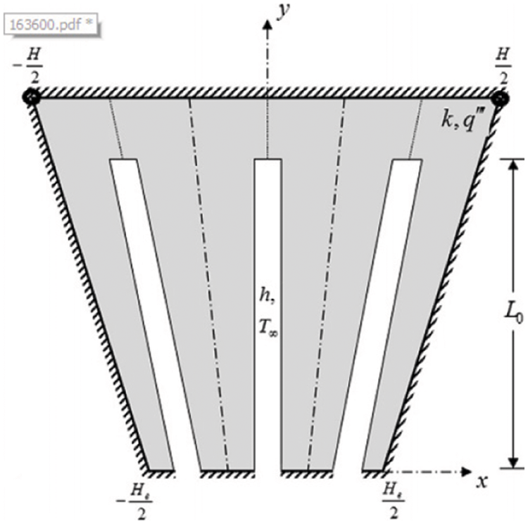
Figure 6: Geometric characteristics of the trapezoidal compartment under the production of internal heat with N internal cavity

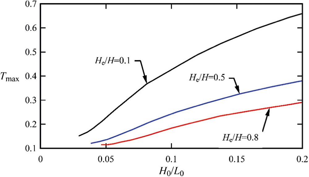
Figure 7: The effect of the parallel parameter H0/H0L0eL0 on the maximum surface temperature for the trapezoidal chamber with the production of internal heat with the homogeneous internal cavity for ( α=∞ , H/HLL=1 and N=1 )

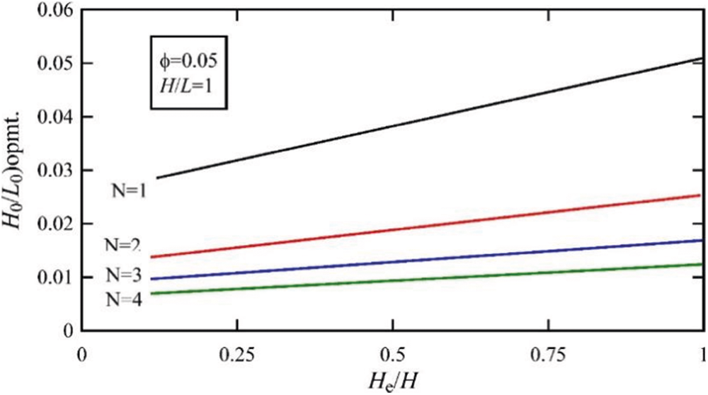
Figure 8: The effect of the number of internal holes, N, on the optimum value of H0/H0L0L0 for a trapezoidal compartment according to He/HeHH

In Figs. 6 and 7, the effect of different parameters of the optimum value of parameter H0/H0L0L0 for a trapezoidal compartment with N internal cavity is shown. In these shapes, we can see the optimal values of H0/H0L0L0 and maximum optimal temperature for the wide range of parameters He/HeHH . According to the results of Fig. 9, it is observed that with increasing number of cavities, the maximum temperature of the system can be significantly reduced.

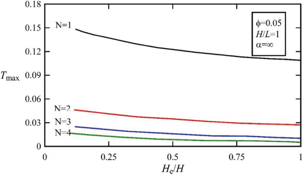
Figure 9: The effect of the number of internal holes, N, on the optimal value of the maximum temperature of the trapezoidal compartment in He/HeHH

3.2 Comparison of the Results of the Present Research Model with the Presented Models

In the preceding sections, optimization results were obtained to minimize the maximum temperature of the system with the cavity presented in this study for the cavity N. In this section, the minimum temperature of the simplified system presented in this study is compared for the optimal state with the results of the models presented in other studies. In fact, this comparison clearly shows the innovation and performance of the simple model presented in this study. For this purpose, in Fig. 8, the comparison between several models in optimal modes for different cocoons of different magnitudes ϕ and α is presented. In this figure, the results are presented for a rectangular box with a constant H/HLL=1 ratio. Two significant results can be seen using the results of Fig. 10. As shown in the results of Fig. 10, for simple cases with N cavities, simplified models provide the maximum system temperature drop compared to the other complex models presented. For example, the minimum system temperature for the enclosure with 3 cavities, 4 cavities and 5 cavities in optimal mode is lower than the value obtained for the compartment with a T-shaped cavity, a T-Y shape and a compartment with a T-Y2 cavity. It should be noted that the production of the compartment with T, Y, T-Y and T-Y2 holes is very complicated and costly. Considering the simple design presented in this study is cost effective and also reduces the maximum temperature of the system than other models, simple systems can replace the other complex cocoons. According to the results of the recent comparison in Fig. 11, the temperature distribution for different samples is compared with the results of the present research models. Also in Table 1, the numerical values of the comparisons performed in Fig. 10 are presented in order to provide a more accurate comparison.

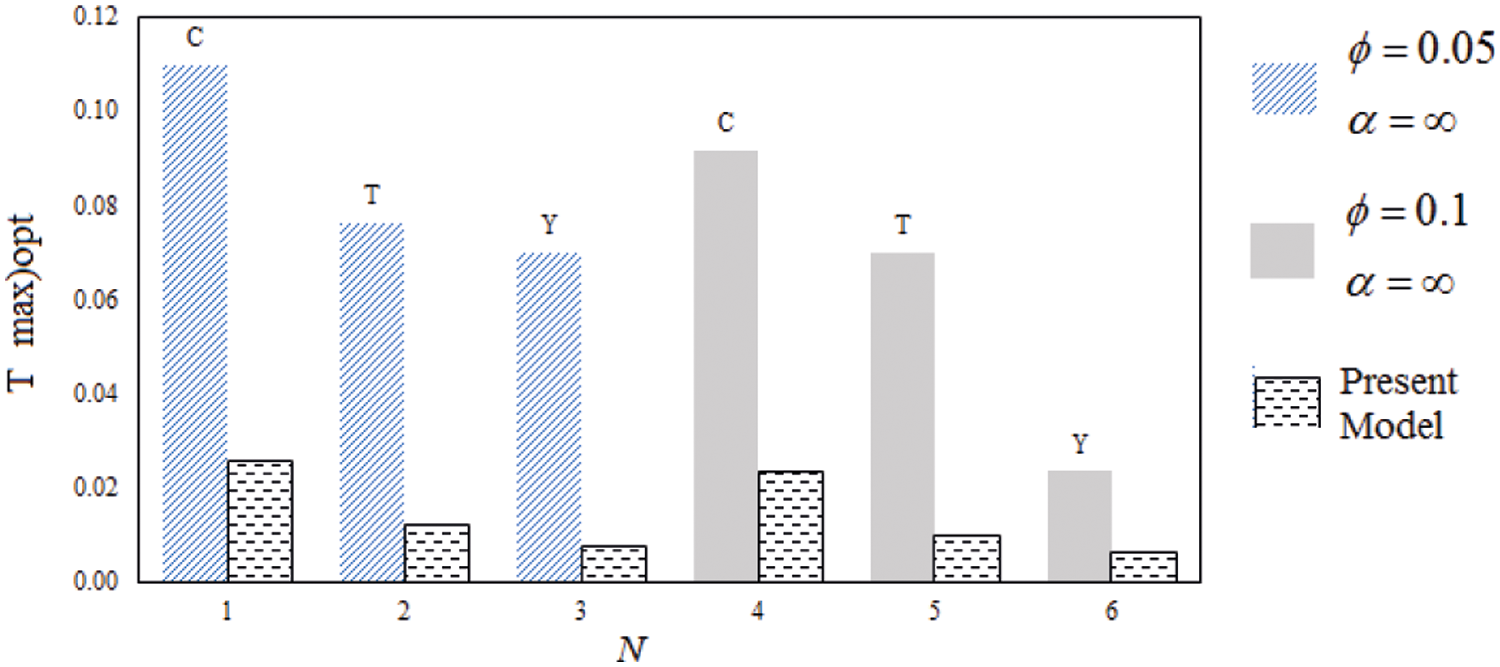
Figure 10: Comparison between several models in optimal modes for different cockpits of different magnitudes ϕ and α

3.3 Providing a New System with a Vein Structure

In this section, we present a new system that combines two types of cavities. In this type of system, a cavity with heat transfer displacement accelerates the cooling process, and the other cavity is used by another material with a higher thermal conductivity to distribute the temperature better at the surface of the object. In Fig. 11, an example of this system is shown. In this case, it is possible to influence the parameters such as ratio η=kp/kpk0k0 and position of the sex with high conductivity coefficient.

Dimensional characteristics of the cavity of the heat exchanger are in accordance with the description of the previous sections. In this section, in order to study the effect of drilling with different conduction resistance, the convexity of the heat transfer surface is considered constant equal to H0/H0L0L0=0.1 and ϕ0=0.05 . In the following, the ratio k~=k0/k0kpkp is considered as the next parameter.

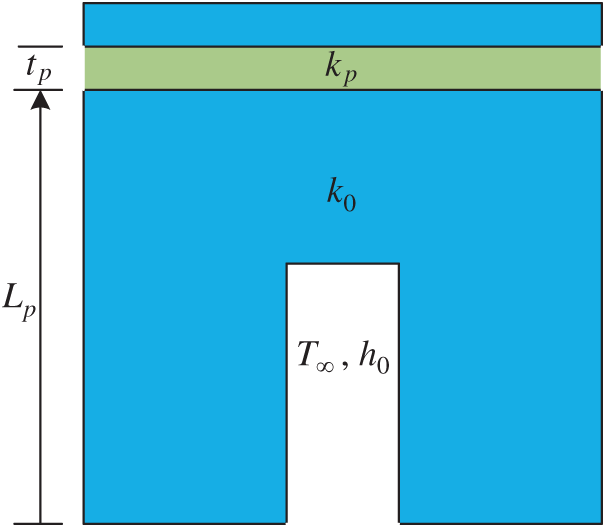
Figure 11: A hybrid system consisting of two different types of holes

In Fig. 12, the distribution of body temperature for α=0.1 and Lp=0.8 in the presence of a cavity with a conductivity coefficient k~=1 and in the absence of it. As you can see, the new design delivers about 25% of the body’s maximum temperature. Accordingly, it can be argued that the proposed design, in addition to having high performance capabilities and ease of implementation, can replace other designs.

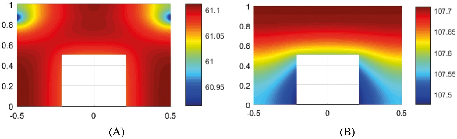
Figure 12: The body temperature distribution for α=0.1 and Lp=0.8 (A) in the presence of a cavity with a conductivity coefficient C and (B) in the absence of it

In order to study the effect of conduction coefficient on system performance, in Fig. 13, the temperature distribution of the object is compared to three values of k~=1 , k~=100 and k~=1000 . As the results show, the coefficient of conductivity of the body does not have a significant effect on the temperature of the solid state of the object, but with increasing the conduction coefficient, the conduction temperature is increased in the object and a greater range of the object at low temperatures continues to function, which is presented is another advantage of the model.

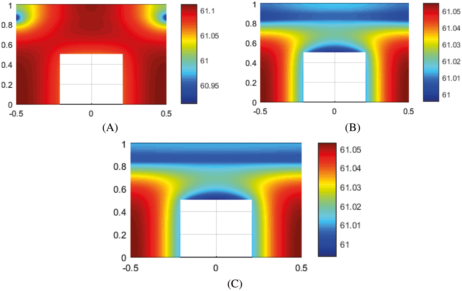
Figure 13: The temperature distribution of the body for three quantities (A) k~=1 , (B) k~=100 and (C) k~=1000

4  Conclusion

The performance of modern electric vehicle Li-ion battery cells depends on the working temperature and state of charge variation during the working loads [21,22]. In this paper based on the study of the operation of the system, a new design was presented as a combination of two cavities with heat transfer and the other with a thermal conductivity coefficient for the battery cooling system. The results show that the distribution of body temperature for α=0.1 and Lp=0.8 in the presence of a cavity with a conductivity coefficient k~=1 and in the absence of it. As it can be seen, the new design delivers about 25% of the body’s maximum temperature. Accordingly, it can be argued that the proposed design, in addition to having high performance capabilities and ease of implementation, can replace other designs in the batteries of electric vehicles. For future studies followings are recommended:

The following is suggested for future work in the continuation of the present study:

- Design and optimization of the structure of cooling ducts in electronic components using structural theory

- Structural design for cooling the surface of a disk using streams of materials with high conductivity

- Design and optimization of conductive tree structures in micro and Nano dimensions for cooling electronic components.

Funding Statement:The authors received no specific funding for this study.

Conflicts of Interest: The authors declare that they have no conflicts of interest to report regarding the present study.

This work is licensed under a Creative Commons Attribution 4.0 International License, which permits unrestricted use, distribution, and reproduction in any medium, provided the original work is properly cited.