| Fluid Dynamics & Materials Processing |
DOI: 10.32604/fdmp.2022.019691
ARTICLE
Optimization of the Structural Parameters of a Plastic Centrifugal Pump in the Framework of a Flow Field Analysis
1School of Mechanical Engineering, Anhui Polytechnic University, Wuhu, 241000, China
2Hohai University, Nanjing, 210098, China
3Anhui Institute of Information Technology, Wuhu, 241199, China
*Corresponding Author: Wenbin Luo. Email: lwbyt08@163.com
Received: 08 October 2021; Accepted: 28 December 2021
Abstract: In order to determine the optimal structural parameters of a plastic centrifugal pump in the framework of an orthogonal-experiment approach, a numerical study of the related flow field has been performed using CFX. The thickness S, outlet angle β2, inlet angle β1, wrap angle, and inlet diameter D1 of the splitter blades have been considered as the variable factors, using the shaft power and efficiency of the pump as evaluation indices. Through a parametric analysis, the relative importance of the influence of each structural parameter on each evaluation index has been obtained, leading to the following combinations: β1 19°, β2 35°, S 2 mm, wrap angle 154°, and D1 85 mm (corresponding to the maximum efficiency of 75.48%); β1 19°, β2 20°, S 6 mm, wrap angle 158°, and D1 81 mm (corresponding to the minimum shaft power of 75.48%). Moreover, the grey correlation method has been applied to re-optimize the shaft power and efficiency of the pump, leading to the following optimal combination: β1 19°, β2 15°, S 4 mm, D1 81 mm, and wrap angle 152° (corresponding to the maximum efficiency of 71.81% and minimum shaft power of 2.187 kW).
Keywords: Plastic centrifugal pump; splitter blade; orthogonal experiment; grey correlation method; optimal combination
In recent years, pumps have been used in various industries, becoming the second most popular machinery [1]. However, most flow channels of centrifugal pumps are long and narrow, leading to high hydraulic loss and disc friction consumption, which has detrimental effects on the operation of the pumps. These problems may be solved by designing splitter blades. Splitter blades can control the “jet-wake” phenomenon at impeller outlets and mitigate congestion at blade inlets. Moreover, splitter blades can alleviate flow separation in impellers so as to reduce uneven flows inside pumps [2].
Geng et al. [3] adopted the quasi-orthogonal experimental method to change the effective flow area ratio of the inlet to the outlet of the flow channel of an ultra-low specific speed centrifugal pump under the condition that the main geometric parameters of the pump remain constant. CFD was used to analyze the effects of different area ratios of the inlet to the outlet on the pump’s performance. Sun et al. [4] established an optimization model concerning the blade shape of a centrifugal pump. The model took the efficiency of the pump as the target function and the distribution coefficient of the inlet attack angle and blade mounting angle as two design variables and then applied the mathematical programming method to seek the optimal blade shape that meets the requirements of the given steam volume and head. Yuan et al. [5–9] used the orthogonal experimental method to study the effects of the geometric parameters of various flow passage components on the performance of a low specific speed pump equipped with splitter blades (or long/short blades, composite blades).
Korkmaz et al. [10] remained the shell, blade inlet angle, blade thickness, blade width, impeller inlet diameter, and impeller outer diameter of a centrifugal pump unchanged and then changed the number of blades and chose splitter blades of different lengths to find the design parameters corresponding to the highest efficiency of the pump. Mustafa et al. [11–13] used the neural network method to analyze the head curves of a deep well pump equipped with different numbers and lengths of splitter blades. The optimal blade design was found, and its best efficiency increased by 6.6%. Al-Obaidi [14] used CFD to study the features of the flow field and pressure pulsation in the time domain and frequency domain in an axial flow pump by varying the impeller blade angle. Flow analysis manifested that the blade angle influences such flow features as static pressure, turbulent kinetic energy (TKE), pressure pulsation, axial velocity, radial velocity, and tangential velocity. Al-Obaidi [15] used CFD to analyze the internal flow field pattern of a centrifugal pump. The results noted that when the impeller rotates near the tongue region, the pressure in this region is higher than in other parts. Moreover, the pressure and velocity variations within the pump increase with the impeller’s rotational speed. Ahmed Ramadhan Al-Obaidi [16] analyzed the flow behavior in an axial flow pump by changing the number of its blades. The numerical results revealed that the blades have significant effects on the pressure, shear stress, magnitude velocity, axial velocity, radial velocity, tangential velocity, and average pressure.
Kergourlay et al. [17] studied the influence of the splitter blades on the internal flow field of a centrifugal pump and discovered that adding splitter blades can increase the head and reduce the pressure pulsation but increase the radial force. Zhang et al. [18–20] performed numerical calculations on the schemes with/without splitter blades or with different splitter blades. The data demonstrated that adding splitter blades can mitigate the congestion at the blade inlet and reduce the pressure of the impeller inlet, volute outlet pressure, and pressure pulsation at the dynamic and static interface, thereby increasing the pump head. Fannian et al. [21] established six numerical models with different blade inlet angles to study the influence of the blade inlet angle on the flow rate of a centrifugal fan. The method based on frozen rotors and realizable k-ε turbulence, with the help of the CFD software, was used to simulate the centrifugal flow. The three-dimensional flow inside the fan revealed how the flow rate of the fan changes with the blade mounting angle. Cheng et al. [22] carried out a numerical simulation of the pump in the framework of the calculation model based on the Reynolds time average N-S equation, the RNG k-ε turbulence method and the SIMPLE algorithm, and evaluated the effects of different guide vane wrap angles on the pump performance, the internal loss of the guide vane and the guide vane. The effect of the flow field distribution in the leafless area of the blade outlet. The results show that the wrap angle has a significant effect. A moderate increase in the wrap angle can improve the flow characteristics and reduce the turbulence loss. Tian et al. [23] considered the four geometric parameters of the impeller’s inlet diameter, inlet width, number of blades and blade angle, and designed the L9 (34) experimental table, calculated the lift and efficiency of the 9 design schemes under the rated flow, and adopted the range The analysis method is used to process and an optimized model is obtained.
In this study, CFX was employed to numerically simulate the flow field of a plastic centrifugal pump. An orthogonal experiment was conducted with such structural parameters as the thickness S, outlet angle β2, inlet angle β1, wrap angle, and inlet diameter D1 of the splitter blades as five factors, taking the shaft power and efficiency as evaluation indices. Through range analysis of the orthogonal experiment, the ranking of the influence of each structural parameter on each evaluation index was obtained. Moreover, the grey correlation method was used to achieve the multi-objective optimization of the shaft power and efficiency.
2 Model Design of the Plastic Centrifugal Pump
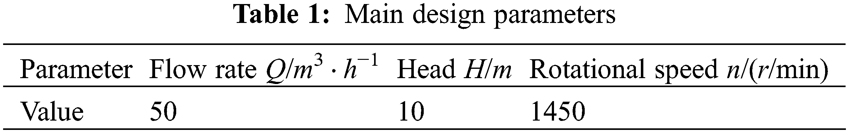
It is a low specific speed centrifugal pump, whose main parameters are listed in Table 1.
The hydraulic design of the pump was the first step in this study, and the structural parameters of the design would significantly affect the pump’s performance [24]. The structural parameters were determined based on the above design parameters Q, H, and n.
(1) Inlet diameter and inlet velocity of the pump
where,
Ds − Inlet diameter (m);
Q − Flow rate (m3/h);
Vs − Inlet velocity (m/s);
Then, the inlet velocity Vs = 2.76 m/s [24], and the inlet diameter Ds = 80 mm.
(2) Outlet diameter and outlet velocity of the pump
The outlet diameter of the pump is calculated according to Eq. (2):
Dd − Outlet diameter (mm).
The connection coefficient is 0.9; then, the outlet diameter Dd = 72 mm.
The outlet velocity is calculated according to Eq. (3):
Vd–Outlet velocity (m/s).
Then, Vd = 3.41 m/s.
(3) Specific speed
ns−Specific speed;
H−Head (m).
Then,
(4) Hydraulic efficiency of the pump
The hydraulic efficiency of the pump is calculated according to Eq. (5):
Then, ηh = 0.86.
(5) Volumetric efficiency of the pump
The volumetric efficiency of the pump is calculated according to Eq. (6):
Then, ηv = 0.97.
(6) Mechanical efficiency of the pump
The mechanical efficiency of the disc friction loss is calculated according to Eq. (7):
Then, ηm = 0.88.
(7) Total efficiency of the pump
The total efficiency of the pump is calculated according to Eq. (8):
Then, η = 0.74.
(8) Shaft power and motor power
The power of the pump is calculated according to Eq. (9):
ρ−Medium density (kg/m3);
g−Acceleration of gravity (m/s2).
where, ρ = 1000 kg/m3, and g = 9.81 m/s2. Then, P = 1.774 kW.
Motor Power
k−Motor margin coefficient; k = 1.1∼1.2;
ηt−Transmission efficiency, with a direct drive motor;
Then, Pc = 2.148 kW.
The motor output torque is calculated according to Eq. (11):
Then, Mn = 14.147(N ⋅ m).
2.2 Main Parameters of the Impeller
The impeller of a centrifugal pump usually takes a semi-open or closed structure. A semi-open impeller has high strength and is easy to shape. Hence, it became the first choice in this study. Its structure is shown in Fig. 1.
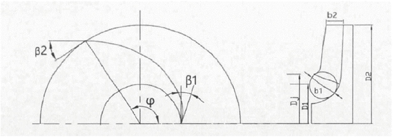
Figure 1: Impeller structure
There are plenty of design methods for the impeller, but the parameters in them do not vary significantly. In this study, the speed coefficient method was applied to calculate the structural parameters of the impeller [24].
(1) Inlet diameter of the impeller
The equivalent diameter of the impeller inlet is calculated according to Eq. (12):
k0-Coefficient,
Then, D0 = 95.568 mm.
The inlet diameter of the impeller is calculated according to Eq. (13):
dh−Hub diameter (mm);
dh is valid only for structural design. For hydraulic design, dh = 0; then,
The blade inlet diameter is estimated as follows:
k1-Coefficient, generally k1 = 0.7 ∼ 1.0;
The coefficient k1 is determined by the specific speed. It takes a larger value for a low specific speed and a smaller value for a high specific speed. According to the specific speed in this study, k1 = 0.85; then, D1 = 85 mm.
(2) Inlet width of the impeller
The inlet width of the impeller is calculated according to Eq. (15):
ξ1−Ratio of the impeller inlet velocity to the inlet diameter.
Generally, ξ1 = 0.9∼1.0; then, substiute D1 = 80 mm, k1 = 0.85 into Eq. (15) to obtain b1 = 25 mm.
(3) Outlet diameter of the impeller
The outlet diameter of the impeller is estimated according to Eqs. (16) and (17):
kD–D2 Correction coefficient.
kD is related to the type and specific speed of the pump. This study’s subject is a single-stage pump, and its specific speed ns = 89.56. Then, substitute
(4) Outlet width of the impeller
The outlet width of the impeller is calculated according to Eqs. (18) and (19):
where,
kb−b2 Correction coefficient.
kb is related to the type and specific speed of the pump. This study’s subject is a single-stage pump, and its specific speed ns = 89.56. Then, substitute
(5) Number of blades
The number of blades according to Eq. (20):
The values of D1, D2, b1, b2 are substituted into Eq. (20). At the same impeller diameter, increasing the number of blades will increase the head without changing the flow rate. Considering the given head H = 10 m, Z = 6.
(6) Inlet and outlet mounting angle of the impeller
In this study, the inlet mounting angle β1 is 19°, outlet mounting angle 33°, and wrap angle 123° [25].
(7) Blade thickness design
The blade is a three-dimensional irregular curved surface, whose accurate thickness was difficult to obtain. For convenience, approximate calculations were used to obtain the blade thickness, then proved by the approximate relationship between geometric figures.
Fig. 2 displays the flow surface, where the shaded part represents the intersection of the blade and the flow surface. Here, a conical surface replaces the irregular flow surface. In this figure, AC represents the flow surface thickness (marked as S); AB represents the circumference thickness (marked as Su). Fig. 3 displays the axial surface, and the axial thickness is marked as Sm. The relationship of these parameters is as follows [26]:
where,
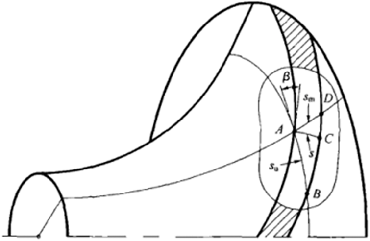
Figure 2: Blade thickness on the flow surface
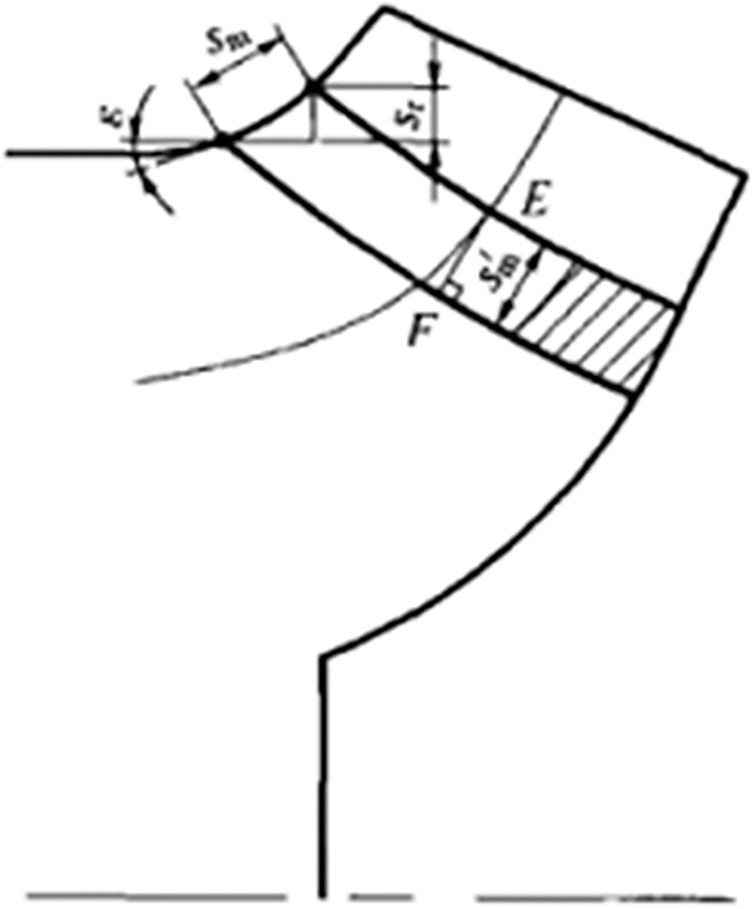
Figure 3: Blade thickness on the axial surface
Sr–Radial thickness;
ε–Angle between the axial streamline and the horizontal plane.
In this study, the inlet mounting angle β1, outlet mounting angle β2, and wrap angle φ were taken from previous studies. The blade profile was obtained through numerically fitting the logarithmic spiral based on the known values and blade profile equation [27].
It can be seen from Eq. (24) that θ is the only unknown quantity. The value of θ ranges from 0 to 123°, which means a series of points can be obtained by changing the value of θ. The blade profile can be obtained by smoothly connecting these points. The number of points reflects the fitting quality. Here, 31 points were selected to plot the blade profile at 4° intervals. The blade profile is as shown in Fig. 4.
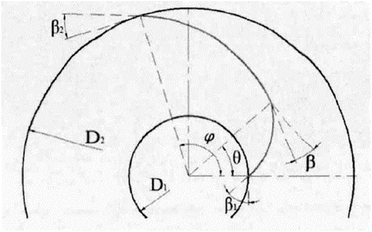
Figure 4: The blade profile
The thinner the blades are, the wider the flow channel is. Then, the slip coefficient is reduced, and the efficiency of the pump is increased. The blades cannot be too thick; otherwise, their strength will be insufficient, and the impeller will deform. Similarly, the thicker the blades are, the narrower the flow channel is. Then, the relative velocity of the fluid in the flow channel becomes larger, and the hydraulic loss is increased. Therefore, in this study, the blade thickness was taken as 2 mm.
2.3 Main Dimensions of the Volute
The flow parts of a pump include an impeller and a volute. The volute is an energy converter. In this study, its main dimensions were designed as follows [25]:
(1) Diameter of the base circle D3
The diameter of the base circle affects the pump’s performance. With D3 to represent the base circle, usually take
For a smaller pump with a high specific speed, take a larger coefficient; similarly, for a larger pump with a low specific speed, take a smaller coefficient. In this study, The diameter of the base circle D3 = 210 mm.
(2) Inlet width of the volute b3
The inlet width b3 of the volute should be determined considering the 8th cross-section, whose shape approaches to be round or square.
Then, b3 = 25 mm.
(3) Mounting angle of the volute tongue
The mounting angle of the volute tongue is represented by φ0. According to [24], φ0 = 22°.
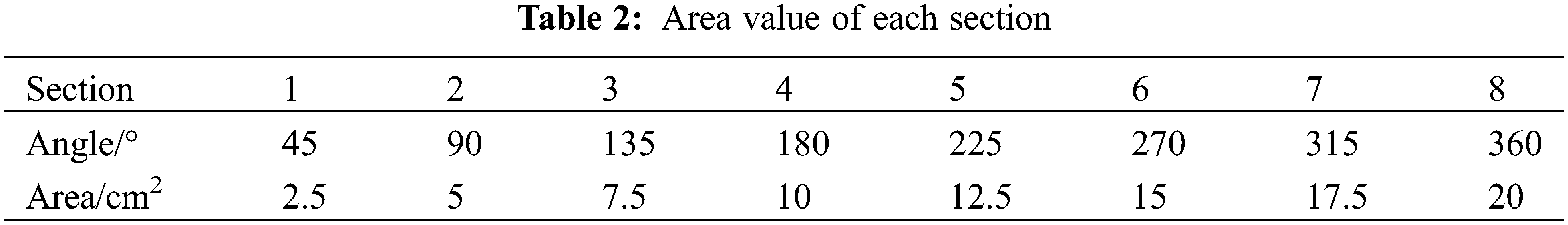
(4) Area of each section
The velocity coefficient method to was applied to calculate the area of each section:
v3−Average velocity of the volute section;
H−Single-stage head of the pump;
k3−Velocity coefficient, the value of which is 0.38 according to [24].
Then, v3 = 6.52 m/s.
The flow through the 8th section is approximately equal to the actual flow of the pump; hence, the area of the 8th section can be calculated by Eq. (28):
The area of other sections are calculated by Eq. (29):
The area of each section was obtained as shown in Table 2.
3 Numerical Simulation Calculations and Flow Field Analysis
The SolidWorks software was used to build the water part of the suction chamber, impeller, and volute of the pump. The inlet and outlet section should be slightly longer to ensure a sufficient flow and reduce the influence of the inlet and outlet section on the water flow so as to improve calculation accuracy. The computational domain model is shown in Fig. 5.
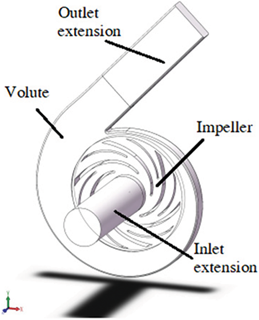
Figure 5: Computational domain model
In this study, ANSYS ICEM CFD was used to mesh the pump model. In ICEM CFD, the design model of the pump imported from the SolidWorks software was processed, and the minimum mesh size was set for the volute, impeller, inlet section, and outlet section, respectively. Because of the complicated computational domain model which consists of a large number of curved parts, these curved parts were divided into unstructured meshes. The meshing steps are shown in Fig. 6, and the results are shown in Fig. 7.
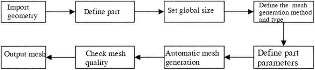
Figure 6: Meshing steps
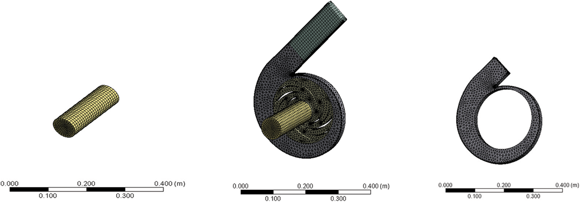
Figure 7: Meshing results
In order to ensure calculation accuracy, there should be enough meshes in the near-wall area to capture the flow in the boundary layer. y+, as a dimensionless parameter [28], representing the distance from the nearest mesh to the wall, is usually used, defined as follows:
The value of y+ is crucial for the selection of the turbulence model. In the numerical simulation of this study, y+ was around 30. In this study, the k-Epsilon model was chosen as the turbulence model to ensure a high quality of meshes [29].
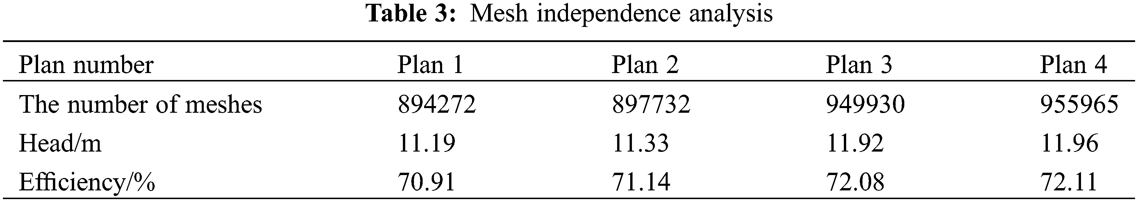
In order to reduce the influence of the number of meshes on calculation results, four different numbers of meshes were obtained, and mesh independence analysis was carried out, as shown in Table 3. It can be seen from Table 3 that with the number of meshes increasing, the variation of the pump head decreases; hence, the influence of the number of meshes on the calculation results can be ignored. The final number of meshes was 949930, the lowest mesh quality was 0.24301, the highest mesh quality was 0.9217, and the average mesh quality was 0.89524.
3.3 Determination of Boundary Conditions and Turbulence Model
3.3.1 Inlet Boundary Condition
The inlet boundary condition is usually set to velocity-inlet or pressure-inlet. The velocity inlet boundary condition applies to incompressible flow issues, and the magnitude and direction of the velocity need to be specified. The pressure inlet boundary condition applies to both compressible and incompressible issues. The relationship between the total pressure P0, static pressure Ps, and fluid velocity u of an incompressible flow are as follows:
The average velocity at the inlet was estimated, and then the static pressure was estimated by Eq. (31).
In this study, the k-ε turbulence model was adopted. It was necessary to set the turbulent kinetic energy k and dissipation rate because a reasonable initial value of each one is beneficial to the convergence of calculations. The following empirical formulas were used to determine the initial values of k and ε:
where, I is the intensity of the turbulence, u is the average velocity at the inlet, L is the characteristic length (in this study, the value is the diameter of the inlet pipe),
3.3.2 Outlet Boundary Condition
The outlet boundary condition is usually set to outflow or pressure-outlet. The outflow boundary condition is applied when the pressure or velocity at the outlet is unknown. In this study, the outlet boundary condition was calculated internally by FLUENT.
3.3.3 Solid-Wall Boundary Condition
Because the Re number of the flow in the near-wall region is low, and the turbulence is not fully developed, such unique ways as the wall function method and low Re number k-ε model are required. In this study, the wall function method was used to solve this problem. The solid wall satisfied the non-slip condition, which indicates the relative velocity W = 0; the pressure was taken as the second boundary condition, namely
The CFX software was applied to read the mesh file as shown in Fig. 8. The inlet boundary condition was Total Pressure and its value was set to 1 atm. The outlet boundary condition was Mass Flow Rate and its value was set to 13.89 kg/s. The rotational speed of the impeller was set to 1450 r/min. The blades and the front and rear cover were all set to Rotating Wall, and their values were 0 rev/min. The Z axis was set to the rotation axis. The wall surface of the extension of the inlet and outlet and the volute was set to No-Slip Wall. Finally, the interface of the impeller and the volute was set to the dynamic-static interface, the interface of the impeller inlet section the dynamic-static interface, and the interface of the volute outlet the static-static interface.
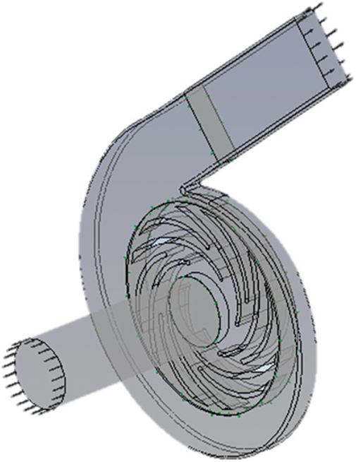
Figure 8: Boundary condition setting
In the simulation software CFX, turbulence models include k-Omega, SST, RNGK-Epsilon, and k-Epsilon. In the k-Epsilon model, the equations are characterized by dissipative scales. Studies have shown that the model can well predict the flow field within fluid machinery. The RNG k-Epsilon model is an improved version of the standard k-Epsilon turbulence model, applying to the turbulence induced by shear motion. Therefore, the k-Epsilon model was chosen for this numerical simulation to predict the flow field.
The turbulent kinetic energy k and dissipation rate ε were used to construct the transport equations as follows:
where, Gk is the generation term of the turbulent kinetic energy k due to the average velocity gradient, and
Continuity equation:
Under normal circumstances:
Assuming that the fluid is not compressible:
Momentum equation (Navier-Stokes equation):
The sum of the various forces acting on the cell from the outside is equal to the rate of change of the momentum of the fluid cell with respect to time.
3.4 Flow Field Analysis of the Pump
In the calculation, the SIMPLEC algorithm was used for the pressure-velocity coupling; the momentum equation, turbulent kinetic energy, and dissipative transport equation were in the second-order windward scheme. In the steady calculation, it converged when the total outlet pressure fluctuated steadily; the unsteady calculation converged when the monitoring results displayed a periodically stable distribution.
In the steady calculation, the “Frozen Rotor” model was used for the two interfaces between the inlet pipe and the impeller and between the impeller and the volute; the General Connection model was used for the interface between the volute and the outlet pipe for they were both stationary. In the unsteady calculation, the “Transient Rotor Stator” model was used for the two interfaces between the inlet pipe and the impeller and between the impeller and the volute, which can capture the interaction between the transient and the stationary state of the rotor in relative motion and take the steady calculation results as the initial conditions for the unsteady calculation [31].
The non-steady time step size Δt is defined as the impeller’s rotational angle at each computational step:
where,
n--impeller’s rotational speed (r/min);
x--the rotational angle of the impeller in each time step.
After setting the boundary conditions, the number of iterations was set to obtain the residual dynamic monitoring process of the internal flow field of the pump. The number of iterations was set to 1000. Fig. 9 shows the residual curves. It can be seen from Fig. 9 that every curve converges when the number of iterations reaches about 300.
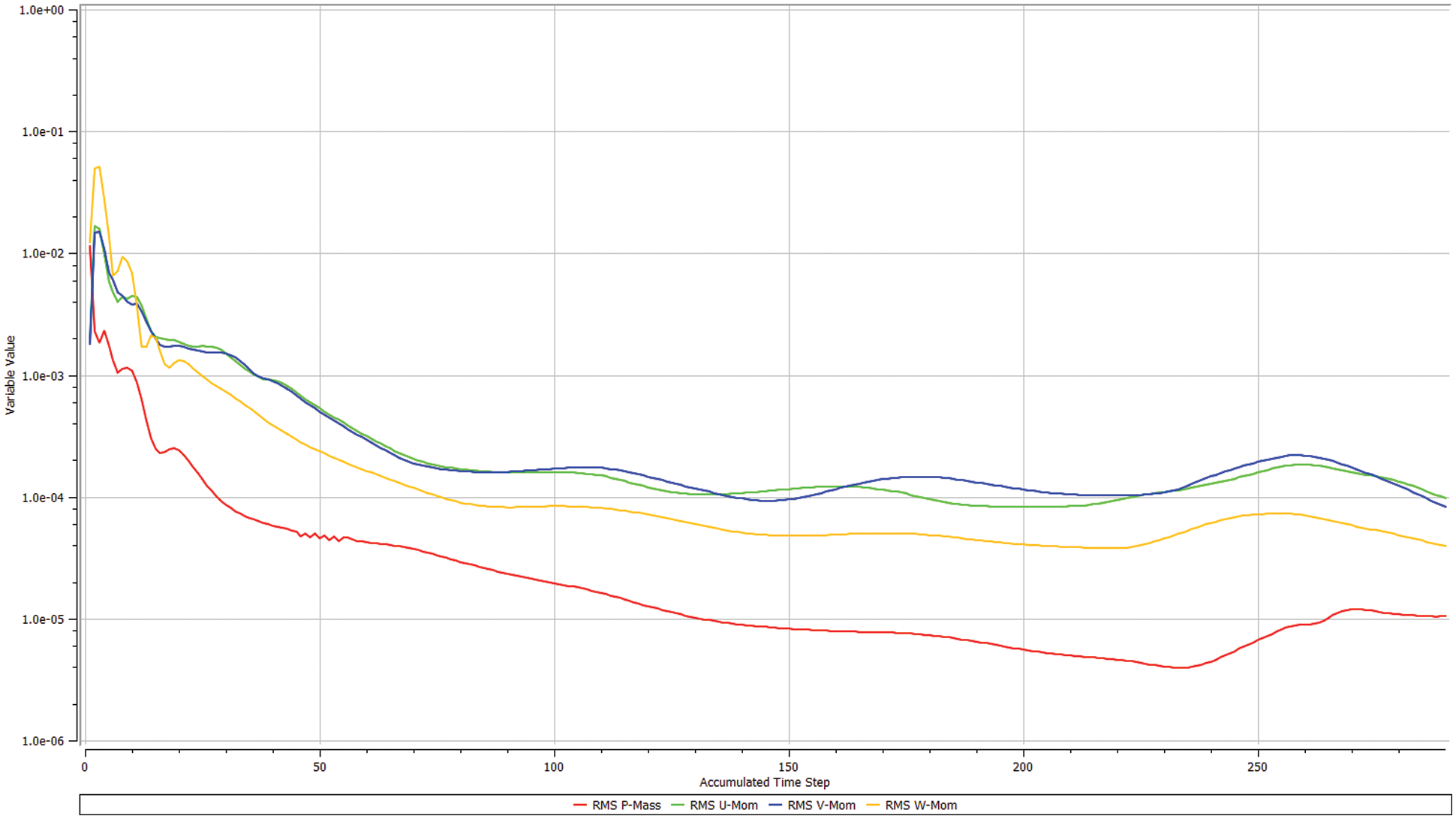
Figure 9: Residual curves
Fig. 10 shows the pressure distribution inside the pump. The pressure gradually increases from the impeller inlet to the outlet, and the pressure at the volute outlet is significantly greater than in other areas of the impeller, which indicates that the liquid from the impeller to the volute is uneven when the impeller is rotating; therefore, vortexes appear between two blades.
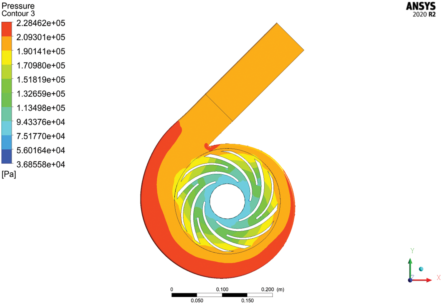
Figure 10: Pressure distribution in the pump
Fig. 11 shows the velocity distribution in the pump. The velocity gradually increases from the impeller inlet to the outlet. Owing to the blades, the flow near the blades is better than far from the center of the blades, and it is relatively far from the center of the blades that vortexes appear.
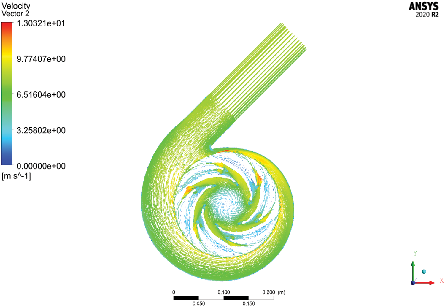
Figure 11: Velocity distribution in the pump
4 Orthogonal Experimental Design of the Structural Parameters of the Pump
4.1 Orthogonal Experimental Design
An orthogonal experiment is a method designed through an orthogonal table standardized by mathematical statistics. It is frequently used to handle multi-factor issues. Its basic steps are as follows:
(1) Determine experimental objectives and indices
When designing an orthogonal experiment for selected parameters, it is necessary to determine its experimental objectives and quality evaluation indices.
(2) Select factors and their levels
In an orthogonal experiment, priority should be given to factors that have more pronounced effects on the quality evaluation indices. The number of levels is usually between 2 to 4 for higher experimental efficiency, and the interval of level values should be reasonable.
4.2 Determination of the Factor Level Values
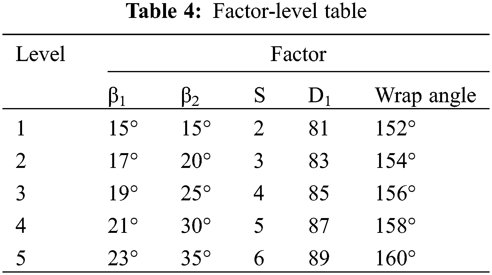
It is impossible to include all factors affecting the efficiency and shaft power of the pump into the orthogonal experiment table. According to relevant theoretical and practical information, the thickness, outlet angle, inlet angle, wrap angle, inlet diameter of the splitter blades were selected as the five factors of the orthogonal experiment. The selected factors and their level values are shown in Table 4. In order to describe the range analysis results clearly, here, A, B, C, D, and E represent the inlet angle β1, outlet angle β2, thickness S, inlet diameter D1, and wrap angle, respectively.
4.2.1 Orthogonal Experimental Results and Range Analysis
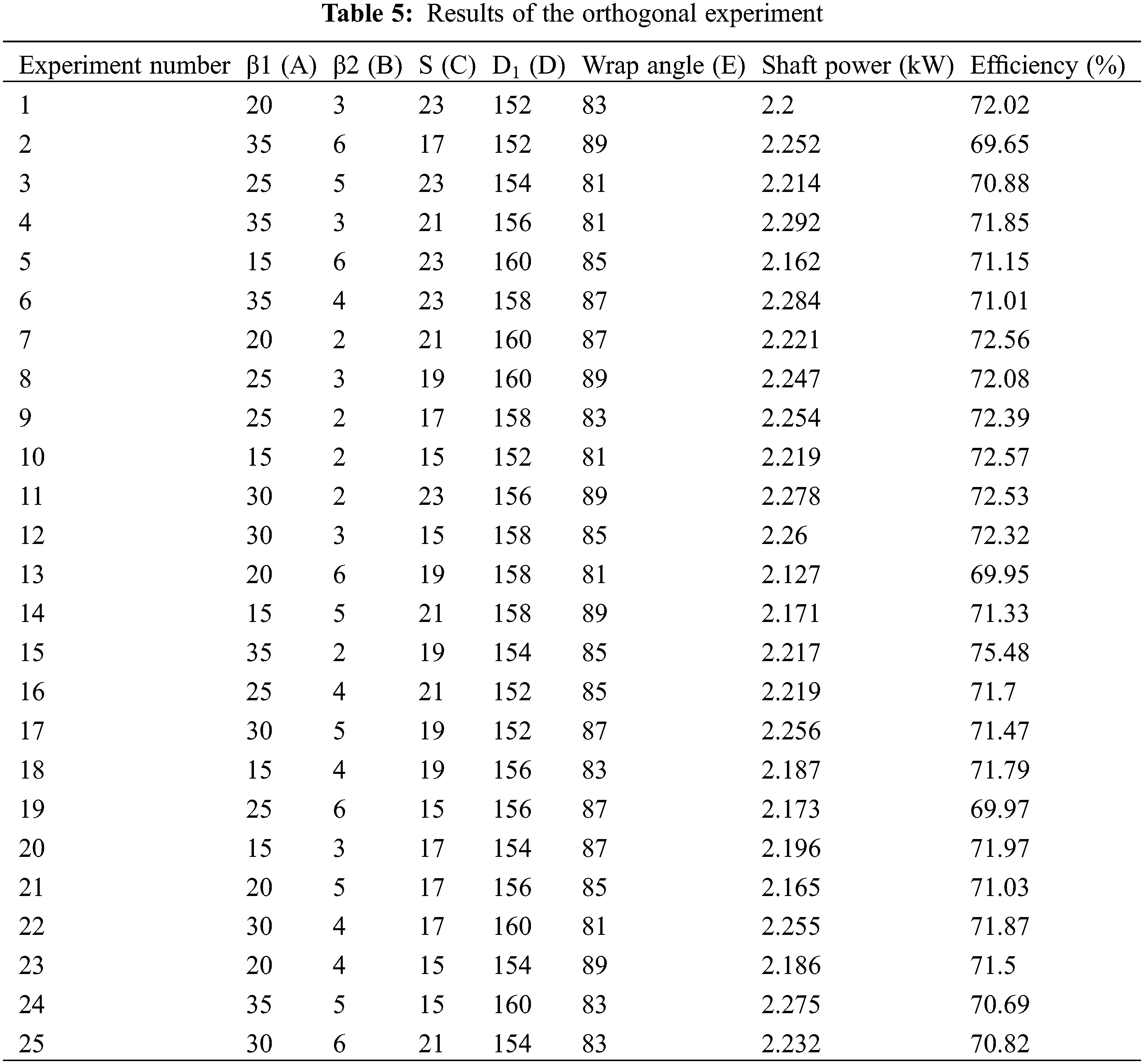
For the five-factor and five-level orthogonal experiment, the orthogonal table was L25 (255). The 25 groups of the orthogonal experiment parameters were numerically simulated separately through the CFX simulation software. The results of the orthogonal experiment are shown in Table 5.
4.2.2 Data Processing of the Experimental Results
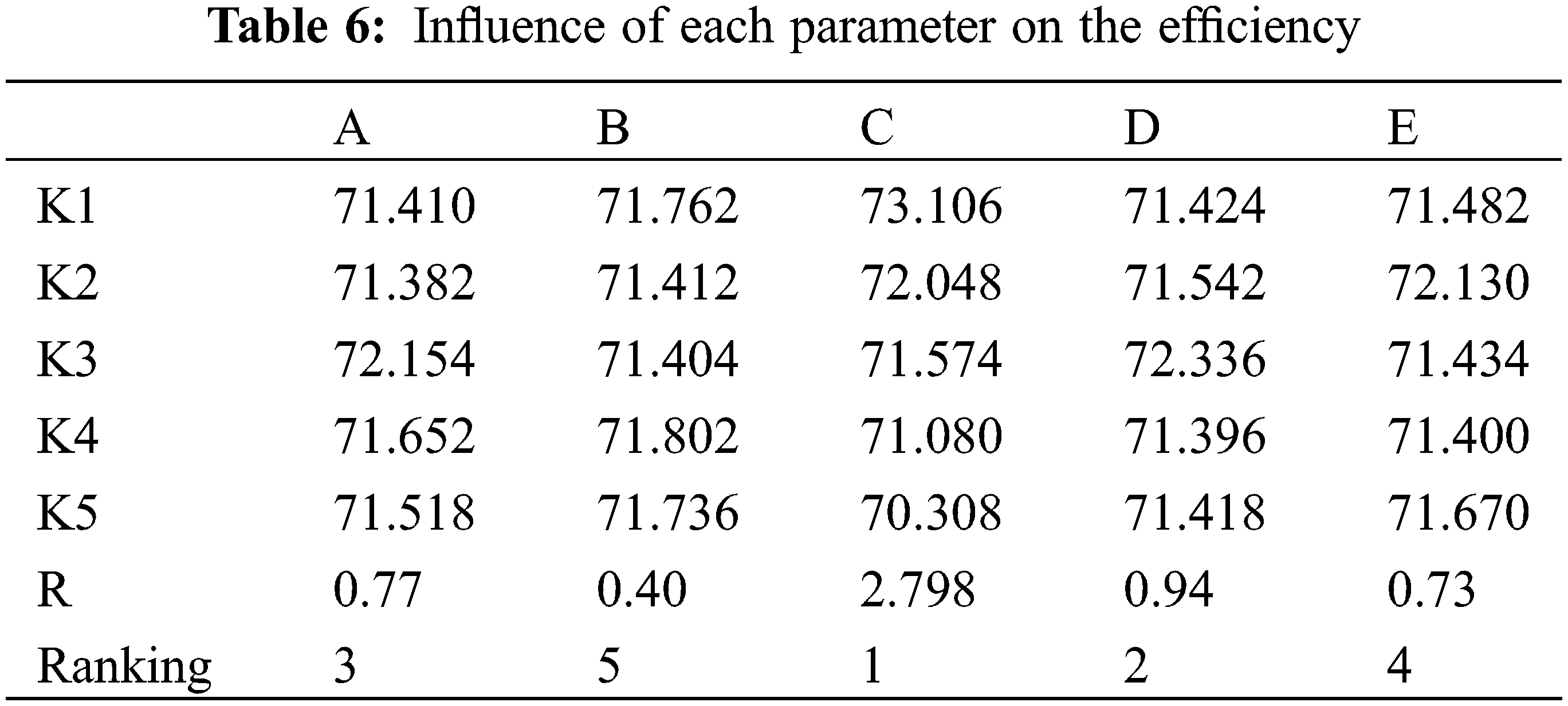
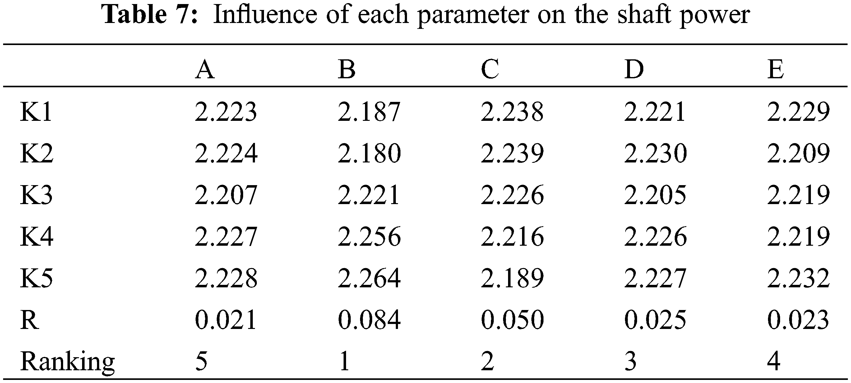
The R value of each parameter was calculated according to the experimental results in Table 5. It can be seen from Tables 6 and 7 that the influence of each factor (structural parameter) on the indices (efficiency and shaft power).
(1) With the efficiency as the evaluation index, the analysis results are shown in Table 6.
(2) With the shaft power as the evaluation index, the analysis results are shown in Table 7.
4.2.3 Analysis of the Experimental Results
1. For the efficiency
In Table 6, Kl, K2, K3, K4, and K5 represent the sum of the efficiency values of each factor at each level. The range R reflects the impact of each factor on the efficiency. Based on the evaluation indices, the best combination was A3B5C1D3E2, where the maximum efficiency was obtained when the inlet angle blade was 19°, outlet angle 35°, thickness 2 mm, wrap angle 154°, and inlet diameter 85 mm.
The orthogonal experiment results were processed by range analysis, and then the ranking of the influence of each factor on the efficiency was obtained as follows: thickness > inlet diameter > inlet angle > wrap angle > outlet angle.
2. For the shaft power
In Table 7, Kl, K2, K3, K4, and K5 represent the sum of the shaft power values of each factor at each level, respectively. The range R reflects the impact of each factor on the shaft power. Based on the evaluation index, the best combination was A4B2C5D4E1, where the minimum shaft power was obtained when the inlet angle was 21°, outlet angle 20°, thickness 6 mm, wrap angle 158°, and inlet diameter 81 mm.
The ranking of the influence of each factor on the shaft power was obtained as follows: outlet angle > thickness > inlet diameter > wrap angle > inlet angle.
5 Multi-Objective Optimization by Grey Correlation Analysis
The orthogonal experiment revealed that when the combination of the structural parameters is A3B5C1D3E2, the efficiency is optimal and that when the combination is A4B2C5D4E1, the shaft power is optimal. However, the range and variance processing only reached the optimum of a single index, and it failed to achieve the simultaneous optimization of multiple goals. Therefore, it was necessary to find a set of structural parameter combinations to optimize the shaft power and efficiency simultaneously. Grey correlation analysis is often used to process data in orthogonal experiments, transforming a multi-objective issue into a single-objective issue that is easier to be analyzed.
Grey correlation analysis is used to obtain the correlation grades between some factors, and the correlation grades reveal the effects and contribution rates of the factors to a system [32]. Its basic principle is to obtain the correlation grades according to the geometric similarity of the curves of the factors. The more similar the curves are, the higher the correlation grades between the factors are.
(1) Construction of the evaluation index matrix
The values of the evaluation indices formed the following evaluation index matrix.
where,
n–Experiment number;
m–Evaluation index number;
Xi(j)-Raw data.
(2) Normalization of the evaluation index data
The dimensions of the raw data were different, and the numerical difference between the factors was large, affecting the model’s accuracy. In order to ensure the equivalence between the indices, it is necessary to normalize the raw data to eliminate their dimensions. The formula of normalization processing is shown in Eq. (48):
(3) Construction of the grey correlation coefficient matrix
Take the maximum value of each index as the reference sequence:
The formula for calculating the grey correlation coefficient is shown in Eq. (51):
The grey correlation coefficient matrix was obtained as follows:
(4) Calculation of the grey correlation grades
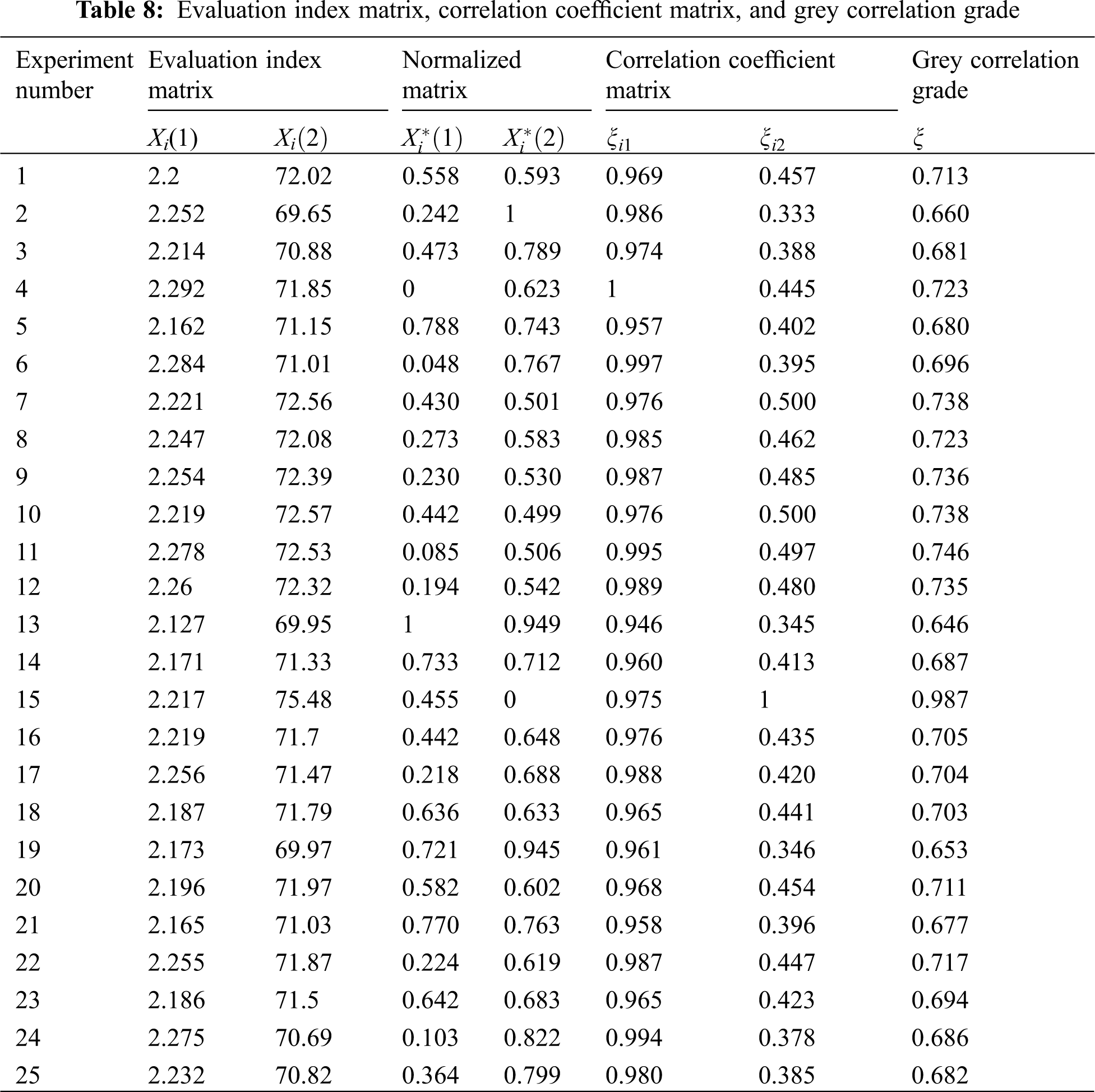
5.2 Grey Correlation Evaluation of the Structural Parameters of the Pump
According to (47) to (53), the grey correlation grades were obtained, and the multi-objective solution was changed to a single-objective solution. The shaft power and efficiency data based on the grey correlation analysis are shown in Table 8.
5.3 Range Analysis of the Grey Correlation Grades
Through range analysis of the grey correlation grades, the mean values and range values were obtained. The larger the value of a factor, the larger the grey correlation grade and the higher the influence on the evaluation indices, as shown in Table 9.
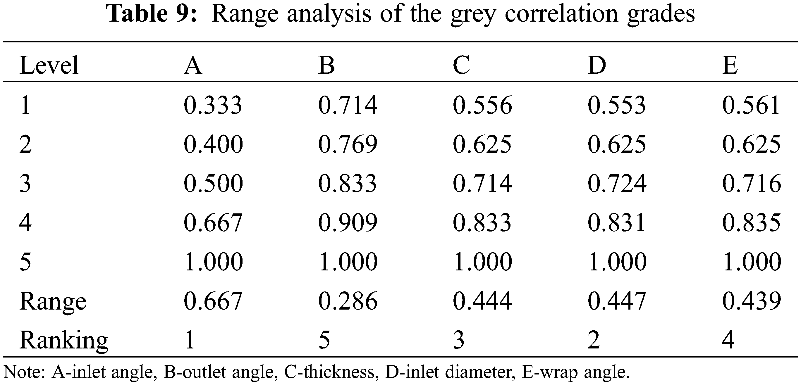
It can be seen from Table 8 that the combination with the largest grey correlation grade is A3B1C3D1E1 (inlet angle 19°, outlet angle 15°, thickness 4 mm, inlet diameter 81 mm, and wrap angle 152°). This combination has the most significant impact on the shaft power and efficiency, and it is the optimal combination of the structural parameters. The CFX software was used to simulate and analyze the combination of the structural parameters, as shown in Fig. 12.
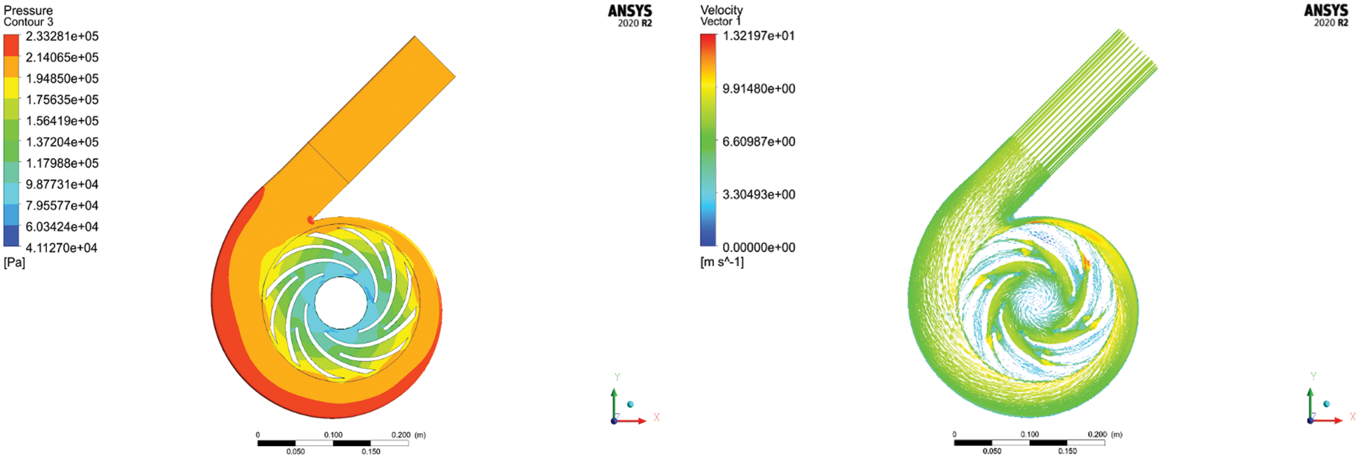
Figure 12: Analysis results of parameter combination A3B1C3D1E1
It can be seen from Fig. 12 that the grey correlation analysis can optimize the structural parameters, and the shaft power and efficiency after optimization are 2.187 kW and 71.81%, respectively.
The structural parameters of the pump were optimized through the orthogonal experiment and grey correlation analysis, and the results are shown in Table 10.
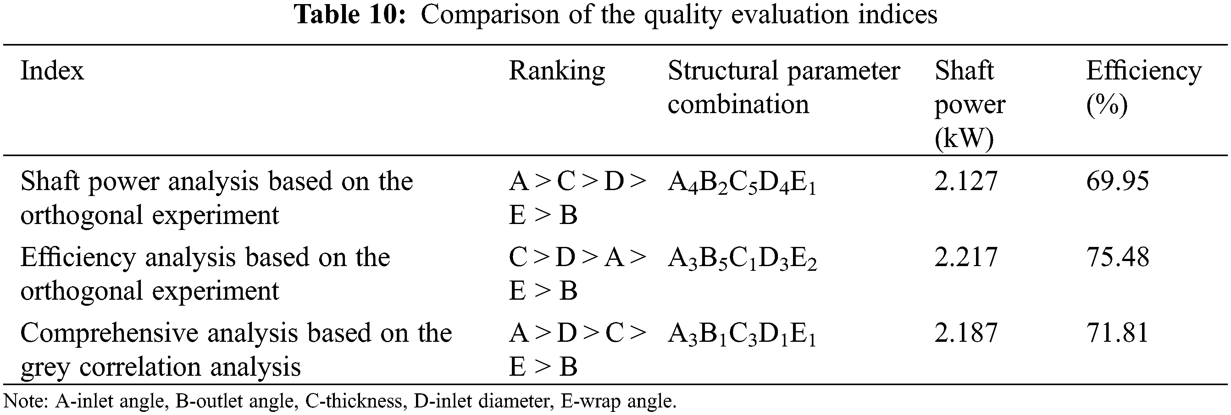
It can be seen from Table 9 that after the structural parameters of the pump were optimized by the orthogonal experiment and grey correlation analysis, different quality index values were obtained. Although neither the shaft power nor the efficiency was optimal among the above three groups of the evaluation indices, they were improved simultaneously. Therefore, it can be concluded that the grey correlation analysis played a role in optimizing the structural parameters of the pump.
The efficiency of plastic centrifugal pumps has become the focus in recent studies, while there has been little research on the shaft power of pumps. In this paper, the structural parameters of a plastic centrifugal pump were calculated and modeled, and numerical simulation analysis of the flow field of the model was performed using CFX, in the framework of an orthogonal experiment. The experiment took such structural parameters as the thickness S, outlet angle β2, inlet angle β1, wrap angle, and inlet diameter D1 of the splitter blades as five factors, using the shaft power of the pump as the primary evaluation index. Through range analysis, the ranking of the influence of each structural parameter on each evaluation index was obtained. Moreover, the grey correlation method was applied to re-optimize the shaft power and efficiency. The conclusions are as follows:
(1) The order of the influence of the five factors on the efficiency is as follows: the splitter blades’ thickness > inlet diameter > inlet angle > wrap angle > outlet angle. When the splitter blades’ inlet angle is 19°, outlet angle 35°, thickness 2 mm, wrap angle 154°, and inlet diameter 85 mm, the maximum efficiency of 75.48% can be obtained;
(2) The order of the influence of the five factors on the shaft power is as follows: the splitter blades’ outlet angle > thickness > inlet diameter > wrap angle > inlet angle. When the splitter blades’ inlet angle is 19°, outlet angle 20°, thickness 6 mm, wrap angle 158°, and inlet diameter 81 mm, the minimum shaft power of 2.127 kW can be obtained;
(3) The grey correlation method was applied to conduct the multi-objective optimization, leading to the following optimal combination of the structural parameters (A3B1C3D1E1): inlet angle 19°, outlet angle 15°, thickness 4 mm, inlet diameter 81 mm, and wrap angle 152°;
(4) Through CFX analysis of the re-optimized model, its shaft power and efficiency were found to be 2.187 kW and 71.81%, respectively. Neither the shaft power nor the efficiency was optimal among the three groups of the evaluation indices, but they were improved simultaneously. Therefore, it can be concluded that grey correlation analysis is conducive to optimizing the structural parameters of plastic centrifugal pumps.
Based on the above conclusions, further research may be conducted from the following aspects:
(1) The shape of splitter blades should be designed based on the impeller of a pump;
(2) The design of splitter blades involves plenty of structural parameters. However, this paper only analyzed the influence of the thickness, inlet diameter, inlet angle, outlet angle, and wrap angle. In the future, more parameters such as the chord length may also be studied.
Funding Statement: This article belongs to the project of the “The University Synergy Innovation Program of Anhui Province (GXXT-2019-004)” “Natural Science Research Project of Anhui Universities (KJ2021ZD0144)” “Wuhu Key R&D Project: Research and Industrialization of Intelligent Control Method of Engine Energy-feeding Hydraulic Semi-Active Mount”.
Conflicts of Interest: The authors declare that they have no conflicts of interest to report regarding the present study.
1. Wang, F. J. (2011). Water pump and water pump station. Beijing: China Agriculture Press. [Google Scholar]
2. Wang, Y. F. (2016). Effects of splitter vanes on internal flow characteristics of low specific speed centrifugal pumps (Master’s Thesis). Jiangsu University. https://kns.cnki.net/KCMS/detail/detail.aspx?dbname=CMFD201602&filename=1016905208.nh. [Google Scholar]
3. Geng, S. J., Nie, C. Q., Huang, W. G., Feng, T., Liu, K. (2006). Numerical study on unsteady flow field of centrifugal pump with different impeller forms. Chinese Journal of Mechanical Engineering, (5), 27–31. DOI 10.3901/JME.2006.05.027. [Google Scholar] [CrossRef]
4. Sun, J. P., Zhang, K. W., Liu, L. Z. (1997). Optimization of the blade shape of centrifugal pump. Journal of Huazhong University of Science and Technology, 25(2), 60–62. [Google Scholar]
5. Yuan, S., Zhang, J., Tang, Y., Yuan, J., Fu, Y. (2009). Research on the design method of the centrifugal pump with splitter blades. Proceedings of the ASME 2009 Fluids Engineering Division Summer Meeting, vol. 1, pp. 107–120.Colorado, USA. ASME. DOI 10.1115/FEDSM2009-78101. [Google Scholar] [CrossRef]
6. Chen, S. S., Zhou, Z. F., Ge, Q. (2005). Orthogonal experiment research on long and short blade centrifugal pumps. Journal of Yangzhou University: Natural Science Edition, 8(4), 45–48. DOI 10.19411/j.1007-824x.2005.04.012. [Google Scholar] [CrossRef]
7. Zhang, J. F. (2007). Research on the numerical prediction and design method of the whole flow field of centrifugal pumps with splitter blades. Zhenjiang: Jiangsu University. [Google Scholar]
8. Yuan, J. P., Li, S. J., Fu, Y. D. (2009). Using orthogonal experiments to study the effect of splitter blades on the performance of centrifugal pumps. Drainage and Irrigation Machinery, 27(5), 306–309. [Google Scholar]
9. Qi, X. Y., Hu, J. X., Tian, Y. B. (2009). Orthogonal design of compound impeller of ultra-low specific speed and high-speed centrifugal pump. Drainage and Irrigation Machinery, 27(6), 341–346. [Google Scholar]
10. Korkmaz, E., Golcti, M., Kurbanoglu, C. (2017). Effects of blade discharge angle, blade number and splitter blade length on deep well pump performance. Journal of Applied Fluid Mechanics, 10(2), 529–540. DOI 10.18869/acadpub.jafm.73.239.26056. [Google Scholar] [CrossRef]
11. Golcu, M. (2001). Analysis of effect to efficiency by adding splitter blade to impeller on deep well pump. Pamukkate University, Denizli Province, Turkey. [Google Scholar]
12. Mustafa, G., Yasar, P., Yakup, S. (2006). Energy saving in a deep well pump with splitter blade. Energy Conversion and Management, 47, 638–651 DOI 10.1016/j.enconman.2005.05.001. [Google Scholar] [CrossRef]
13. Mustafa, G. (2006). Neural network analysis of head-flow curves in deep well pumps. Energy Conversion and Management, 47, 992–1003. DOI 10.1016/j.enconman.2005.06.023. [Google Scholar] [CrossRef]
14. Al-Obaidi, A. R. (2021). Analysis of the effect of various impeller blade angles on characteristic of the axial pump with pressure fluctuations based on time- and frequency-domain investigations. Iranian Journal of Science and Technology, Transactions of Mechanical Engineering, 45, 441–459. DOI 10.1007/s40997-020-00392-3. [Google Scholar] [CrossRef]
15. Al-Obaidi, A. R. (2021). Numerical investigation on the effect of various pump rotational speeds on performance of centrifugal pump based on CFD analysis technique. International Journal of Modeling, Simulation, and Scientific Computing, 12(5). [Google Scholar]
16. Al-Obaidi, A. R. (2020). Investigation of the influence of various numbers of impeller blades on internal flow field analysis and the pressure pulsation of an axial pump based on transient flow behavior. Heat Transfer, 49(4), 2000–2024. DOI 10.1002/htj.21704. [Google Scholar] [CrossRef]
17. Kergourlay, G., Younsi, M., Bakir, F., Rey, R. (2007). Influence of splitter blades on the flow field of a centrifugal pump: Test-analysis comparison. International Journal of Rotating Machinery, 2007,13 . DOI 10.1155/2007/85024. [Google Scholar] [CrossRef]
18. Ye, L., Yuan, S., Zhang, J., Yuan, Y. (2011). Effects of splitter blades on the unsteady flow of a centrifugal pump. Proceedings of the ASME 2012 Fluids Engineering Division Summer Meeting Collocated with the ASME 2012 Heat Transfer Summer Conference and the ASME 2012 10th International Conference on Nanochannels, Microchannels, and Minichannels, vol. 1, pp. 435–441. Puerto Rico, USA. ASME. DOI 10.1115/FEDSM2012-72155. [Google Scholar] [CrossRef]
19. Zhang, J. F., Yuan, Y., Ye, L. T. (2011). Research progress of centrifugal impeller machinery with splitter blades. Fluid Machinery, 39(11), 38–44. [Google Scholar]
20. Zhang, J. F., Ye, L. T., Yuan, S. Q. (2013). The influence of splitter blades on the radial force characteristics of centrifugal pumps. Journal of Agricultural Mechanization Research, 35(10), 181–185. DOI 10.13427/j.cnki.njyi.2013.10.004. [Google Scholar] [CrossRef]
21. Meng, F., Wang, L., Xie, G., Zhao, F., Zhang, D., Du, W. (2017). Effects of blade inlet angle on flow field of centrifugal fan. DEStech Transactions on Engineering and Technology Research, 138–143. DOI 10.12783/dtetr/icmeca2017/11924. [Google Scholar] [CrossRef]
22. Cheng, X. R. (2019). Analysis of the impact of the space guide vane wrap angle on the performance of a submersible well pump. Fluid Dynamics & Materials Processing, 15(3), 271–284. DOI 10.32604/fdmp.2019.07250. [Google Scholar] [CrossRef]
23. Peng, T. (2019). Optimization of a centrifugal pump used as a turbine impeller by means of an orthogonal test approach. Fluid Dynamics & Materials Processing, 15(2), 139–151. DOI 10.32604/fdmp.2019.05216. [Google Scholar] [CrossRef]
24. Guan, X. F. (2011). Modern pump theory and design. Beijing: China Aerospace Publishing House. [Google Scholar]
25. Zhang, Y. Y. (2019). Research on the influence of the blade placement angle of the plastic centrifugal pump on the pump performance based on fluid-structure coupling (Master’s Thesis). Anhui Polytechnic University. https://kns.cnki.net/KCMS/detail/detail.aspx?dbname=CMFD201902&filename=1019052636.nh. [Google Scholar]
26. Liu, M. W. (2020). Research on the effect of impeller blade thickness on pump performance based on fluid-structure coupling (Master’s Thesis). Anhui Engineering University. https://kns.cnki.net/KCMS/detail/detail.aspx?dbname=CMFD202101&filename=1021016850.nh. [Google Scholar]
27. Yan, J., Zhang, J. Y., He, M., Wang, T. (2008). The profile equation of the cylindrical blade with controllable wrap angle of centrifugal pump. Drainage and Irrigation Machinery, (5), 46–49. [Google Scholar]
28. Zhang, D. S., Wu, S. Q., Shi, W. D. (2013). Application and verification of different turbulence models in the simulation of axial flow pump tip leakage vortex. Transactions of the Chinese Society of Agricultural Engineering, 29(13), 46–53. [Google Scholar]
29. Li, X. J., Yuan, S. Q., Pan, Z. Y. (2012). Implementation and application evaluation of boundary layer grid for centrifugal pumps. Transactions of the Chinese Society of Agricultural Engineering, 28(20), 67–72. DOI 10.6041/j.issn.1000-1298.2013.07.010. [Google Scholar] [CrossRef]
30. Muslafa, G. (2006). Neural network analysis of head-flow curves in deep well pumps. Energy Conversion and Management, 47, 992–1003. [Google Scholar]
31. Pei, J. (2013). Transient hydraulic excitation of centrifugal pump, fluid-solid coupling mechanism and unsteady flow strength research (Ph.D. Thesis). Jiangsu University, China. [Google Scholar]
32. Xu, Y., Qin, B. (2015). Research on optimization of injection molding process parameters based on particle swarm optimization BP. Inner Mongolia Science and Technology and Economy, (17), 73–74. [Google Scholar]
 | This work is licensed under a Creative Commons Attribution 4.0 International License, which permits unrestricted use, distribution, and reproduction in any medium, provided the original work is properly cited. |