| Fluid Dynamics & Materials Processing |
DOI: 10.32604/fdmp.2022.018012
ARTICLE
Calculation of the Gas Injection Rate and Pipe String Erosion in Nitrogen Drilling Systems
1China United Coalbed Methane Corporation, Ltd., Beijing, 100011, China
2School of Engineering and Technology, China University of Geosciences (Beijing), Beijing, 100083, China
*Corresponding Author: Hao Yang. Email: yanghao@cugb.edu.cn
Received: 23 June 2021; Accepted: 17 August 2021
Abstract: Detailed information is provided for the design and construction of nitrogen drilling in a coal seam. Two prototype wells are considered. The Guo model is used to calculate the required minimum gas injection rate, while the Finnie, Sommerfeld, and Tulsa models are exploited to estimate the ensuing erosion occurring in pipe strings. The calculated minimum gas injection rates are 67.4 m3/min (with water) and 49.4 m3/min (without water), and the actual field of use is 90–120 m3/min. The difference between the calculated injection pressure and the field value is 6.5%–15.2% (formation with water) and 0.65%–7.32% (formation without water). The results show that the Guo model can more precisely represent the situation of the no water formation in the nitrogen drilling of a coal seam. The Finnie, Sommerfeld, and Tulsa models have different sensitivities to cutting densities, particle size, impact velocity and angle, and pipe string hardness.
Keywords: Coalbed methane; nitrogen drilling; minimum gas injection rate; erosion of pipe string; analysis on the scene
Two prototype wells in a coalbed methane exploration area are studied, which should be regarded as the first directional (Well D) and horizontal (Well H) wells in the world to implement nitrogen drilling technology in coal seams. The amount of gas injection is one of the important design parameters of this process. The amount of gas injection is too small to meet the requirements of carrying rock and liquid, and excessive gas injection will lead to the erosion of the pipe string and the expansion of the wellbore. The reasonable calculation of the gas injection rate has important guiding significance for on-site gas injection volume, equipment selection, and drilling speed.
Angel [1] first proposed the calculation method of minimum gas injection rate in air drilling. The model adopts the Weymouth friction coefficient, which is suitable for a smooth pipe wall, while the actual wellbore is relatively rough. The temperature has a great influence on the air, and the simple use of average temperature in the calculation process will lead to inaccurate results. The minimum gas injection rate calculated by this model is 20%–30% lower than the actual value in the field [2,3].
Based on the Angel model, Guo et al. [4] proposed a widely used minimum gas injection calculation model. In this model, the friction factor coefficient of Nikuradse is introduced into the Angel model to make it suitable for relatively rough boreholes. The actual temperature is used to replace the average temperature, and the inclination angle is introduced into the model to calculate the minimum gas injection rate in the straight, inclined, and horizontal sections [5–8].
Assuming that polygonal abrasive particles impact the surface of a plastic target at a certain speed and angle, Xu [9] proposed the micro-cutting model theory of erosion wear, which resulted in target wear. Experiments show that the model can suitably explain the erosion wear of plastic materials under multi-angle abrasive and low angle impact. However, it shows that the erosion wear of brittle materials, a high angle of attack, and non-polygonal abrasive grains (spherical abrasive grains) exhibits great error.
Taji et al. [10] established a particle collision model. This model assumes that the particles do not rotate, slip, or adhere in the process of colliding with each other. It only considers the changes of the relative motion velocity, particle size, and the number of particles, it ignores the influence of the strong turbulent flow of the fluid itself on the collision of particles.
International University proposed the erosion wear model [11], which includes target properties, particle shape, as well as the particle impact velocity and angle. The model has many parameters, and the rough estimation of parameters also limits its application.
The erosion wear model proposed by Tulsa University includes target properties, particle shape, particle impact velocity, and angle, among others [12]. The model has many parameters, and the rough estimation of parameters also limits its application.
At present, the theory and method of the Guo model are mostly used in the calculation of gas injection rate in gas drilling. Different erosion models have a great influence on the research and analysis of the erosion phenomenon, so it is necessary to analyze the erosion of pipe string according to actual working conditions [13–16]. For Wells D and H that implement nitrogen drilling technology in coal seams in areas with abundant rainfall, this paper uses the Guo model to calculate the gas injection volume and gas injection pressure of the two wells, and uses the Finnie model, Sommerfeld model, and Tulsa model to analyze the erosion of string.
The lower part of the Longtan formation in this exploration area is composed of thin to medium-thick bedded limestone, fine sandstone, and siltstone, with great lithology variation and rich water content. However, the upper part of the Changxing formation is comprised of siltstone and fine sandstone with a thin layer of little limestone, which is rich in water. The exploration area is controlled by the local tensile stress field and is a fault connected with the karst aquifer of the Maokou Formation (P1m), which can replenish the groundwater of the coal measures strata.
Wells D and H are coalbed methane development wells, so nitrogen drilling technology is implemented in the coal seam. The completion depth of Well D is 882 m (casing completion 711 m, open hole completion 171 m), and is 50 m below the coal seam completion. The completion depth of Well H is 1019.57 m (casing completion 917.74 m, open hole completion 101.83 m), and the footage of the coal seam horizontal section reaches 300 m. The combination of drilling tools used in the two wells is presented in Table 1, the gas drilling equipment is shown in Table 2, and the well trajectory is exhibited in Fig. 1.
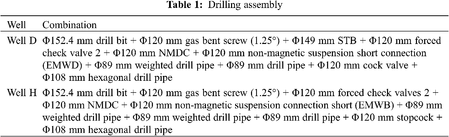
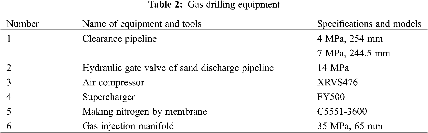
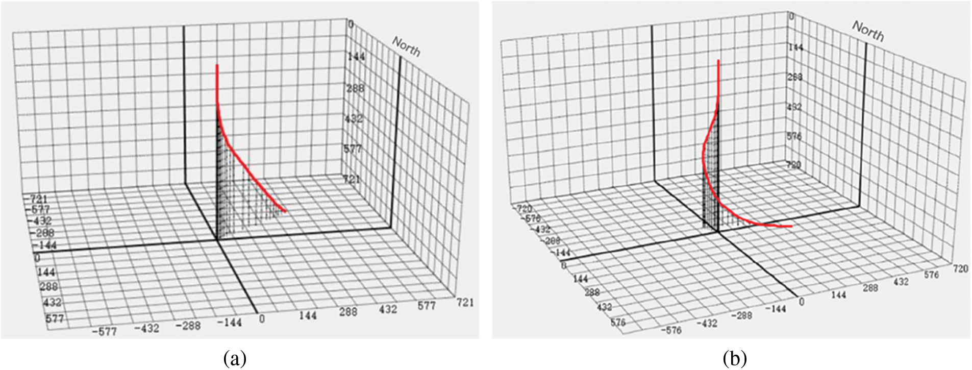
Figure 1: Three-dimensional diagram of well trajectory (a) Well D (b) Well H
3 Minimum Gas Injection Calculation
According to the Guo model [4], the gas injection parameters are calculated as follows:
For the vertical interval, the calculation equation is:
where Sg is the density of gas relative to air; Ts is ground temperature, °R; G is geothermal gradient, °C/m; H is the calculated well depth, ft; Qg0 is the volume flow of gas under standard conditions (14.7 psi, 60 °F), ft3/min;
For inclined and straight sections, the pressure calculation equation at depth H is as follows:
In which, Is is the slant angle of the deviated hole, rad.
For the directional interval, the pressure calculation equation at depth h is as follows:
In the formula, PK is the pressure at the kick-off point, lb/ft2; R is the radius of curvature, ft; Tav is the average temperature of the interval, °R; and I is the angle of inclination, rad.
In formulas (1)–(3):
In the formula,
The calculation method is as follows: first, assume the Qg0 value to get the a and b values; bring the values of a and b into formulas (1)–(3); if the equation holds, the assumed Qg0 is the desired value; otherwise, continue to calculate on the assumption of the Qg0 value.
The basic parameters of Well D and Well H are shown in Table 3.
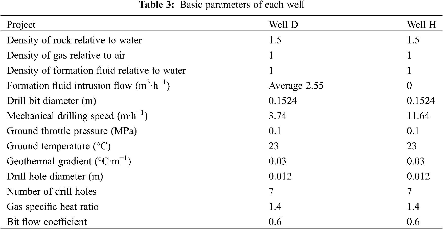
The gas injection volume and pressure are calculated by the Guo model, and the results are shown in Table 4.
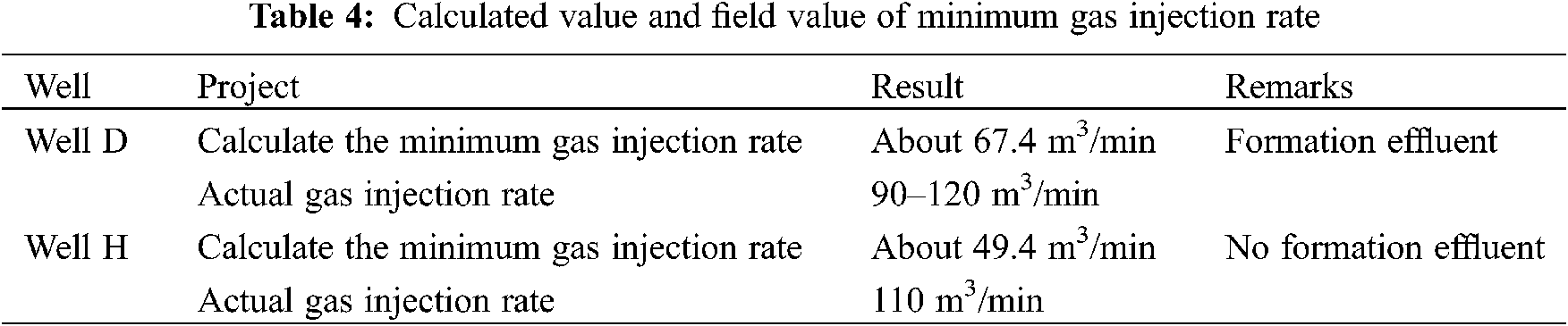
The required gas injection rate of Well D is higher than that of Well H. This is because there is the formation of water in the drilling process of Well D, and the water output of some sections is large. The calculated minimum gas injection volume of the two wells is less than the actual value in the field because the treatment of wellbore roughness in the Guo model cannot fully express the nitrogen drilling in the coal seam.
4 Calculation of Injection Pressure
Combined with Qg0 and the a and b values, the pressures at different positions in the wellbore can be calculated.
For the vertical interval, the upstream pressure is calculated by the following formula:
In which, G is the geothermal gradient, °C/m. For the ± number in the formula, ‘+’ is for the upwelling, whereas the downflow uses ‘−’.
For non-horizontal vertical sections, upstream pressure is calculated using the following formula:
In which, S is the interval length, ft.
For the horizontal interval, the following formula is adopted for calculation:
For the arc hole section, the upstream pressure is calculated by the following formula:
where Im is the maximum dip angle (bottom hole), rad; and R is the radius of curvature of the well section, ft.
The critical pressure ratio of bit water hole is calculated as follows:
In which, Pdn is the downstream pressure, bbl/ft2; Pup is the upstream pressure, bbl/ft2; and k is the specific heat of the gas.
When the velocity of the drill hole is subsonic, the gas flow rate is:
In the formula, C is the flow coefficient, the nozzle of the bit is about 1, and the water hole of the bit body is 0.6.
The relevant parameters at different positions of Well D and Well H are taken to calculate the injection pressure and compare it with the measured injection pressure, as shown in Tables 5, 6, Figs. 2, and 3.
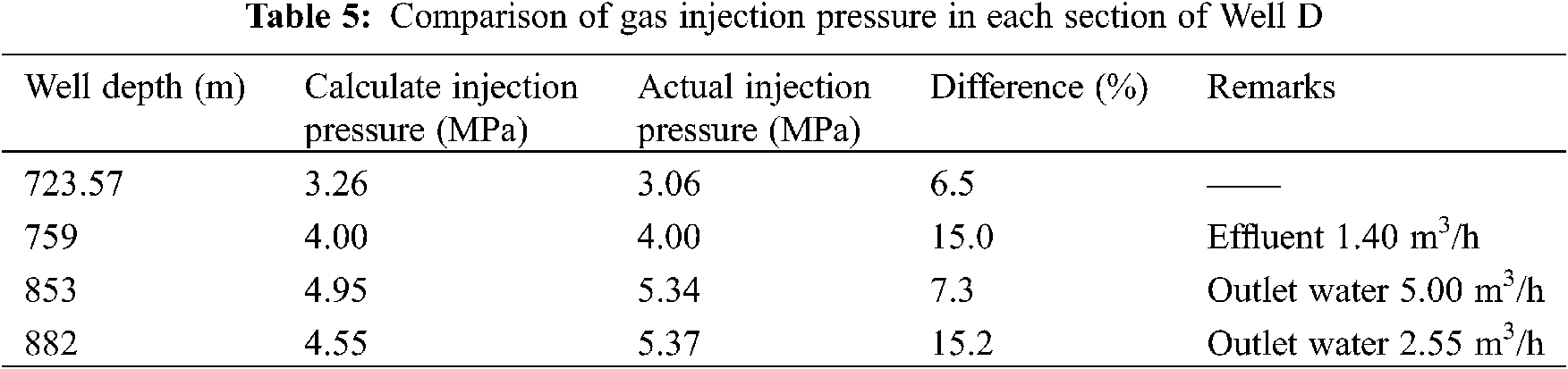

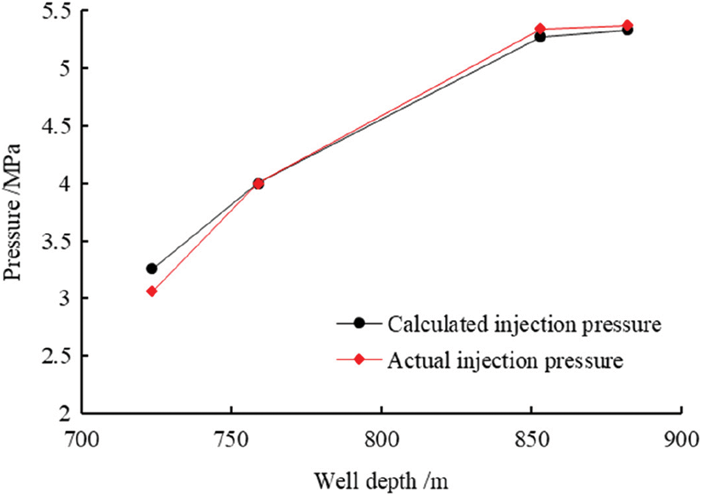
Figure 2: Comparison of gas injection pressure in Well D
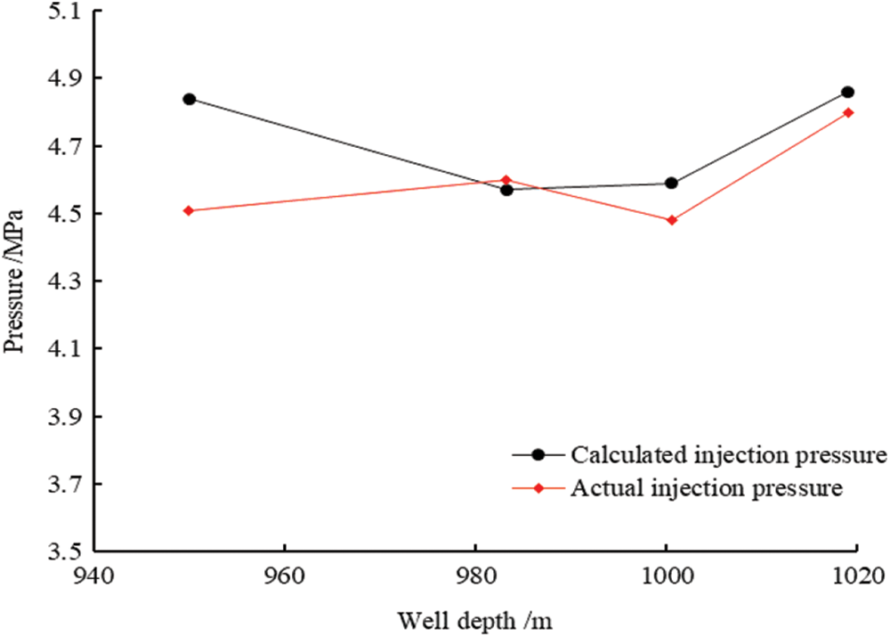
Figure 3: Comparison of gas injection pressure in Well H
The comparison results show that the difference between the calculated injection pressure and the field value is up to 6.5%–15.2%. In the case of no effluent, the difference between the calculation results and the field values is small, which is 0.65%–7.32% and relatively consistent. For nitrogen drilling in the coal seam, the Guo model can better predict injection pressure without water.
5 Calculation of Erosion of Pipe String
The column erosion calculation method is as follows [17–19]:
In which R is erosion rate, kg/(m2·s); C(dp) is a function of the cuttings particle size; f(α) is a function of impact angle; vp is the velocity of cuttings relative to the wall, m/s; b(v) is a function of the relative velocity of cuttings;
The input parameters of the Finnie model are c(dp) = 1.8 × 10⁻⁹, f(α) = 1, and b(v) = 0.
The input parameters of the Sommerfeld model are C(dp) = 1.8 × 10⁻⁹, f({0, 20, 30, 45, 90}) = {0, 0.8, 1, 0.5, 0.8}, and b(v) = 2.6.
The input parameters of the Tulsa model in the above formula are:
where
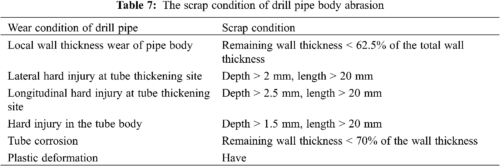
According to the relevant requirements in the standard SY/T5956-2004 “Technical conditions for scrapping drilling tools” and SY/T 5369-2012 “The management and use of oil drill pipe, drill pipe, drill collar” [20,21], the scrapping conditions of drilling tool erosion are shown in Table 7.
5.1 Impact Angle on Erosion Rate
The average particle size of cuttings is 0.26 mm, the impact velocity is 21.74 m/s, and the density is 1500 kg/m3. The Boolean hardness of the column is 260, and the relationship between the erosion rate and the impact angle is plotted in Fig. 4. The erosion rate calculated by the Sommerfeld model and the Tulsa model is the largest when the impact angle is 30°, whereas the Finnie model does not change.
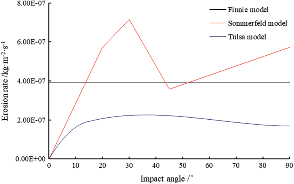
Figure 4: Influence of impact angle on erosion rate
5.2 Impact Velocity of Cuttings on Erosion Rate
The impact angle of cuttings was set to be 18°, the average particle size was 0.26 mm, and the density was 1500 kg/m3. The Boolean hardness of the pipe column was 260, and the relationship curve between the erosion rate and the impact velocity of cuttings is presented in Fig. 5. It can be seen that the erosion rate calculated by each model increases with the increase of the debris impact velocity. The calculation results of the Sommerfeld model are much larger than those of other models.
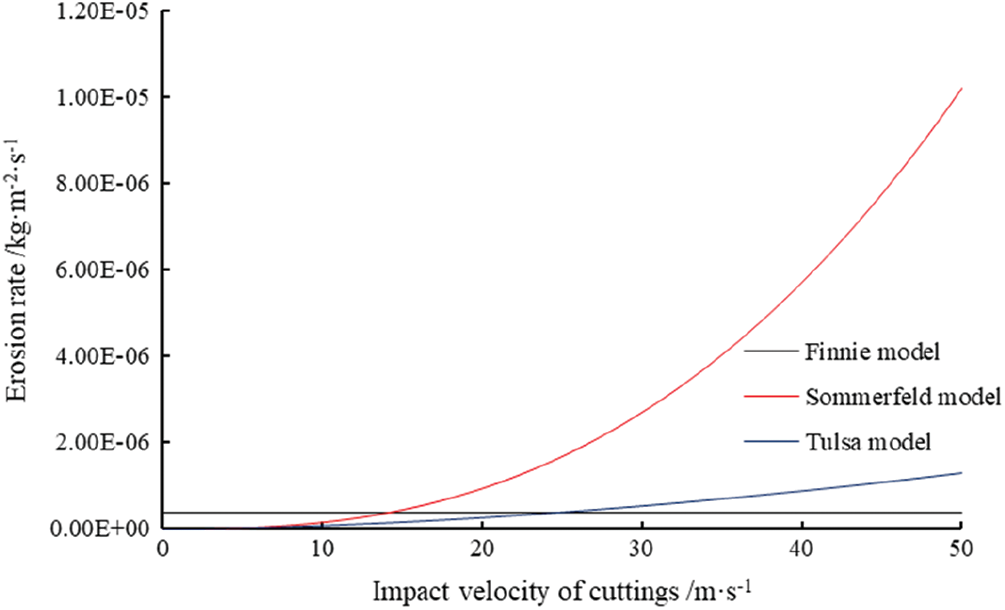
Figure 5: Influence of cuttings impact velocity on erosion rate
5.3 Influence of Average Particle Size of Cuttings on Erosion Rate
When the impact angle of cuttings was set at 18°, the impact velocity was 21.74 m/s at the drill collar and the density was 1500 kg/m3. The Boolean hardness of the string was 260. The relationship curve between the erosion rate and average particle size of cuttings is presented in Fig. 6. It can be seen that the erosion rate calculated by each model increases with the increase of the average particle size of cuttings. The calculation results of the Tulsa model are much larger than those of other models.
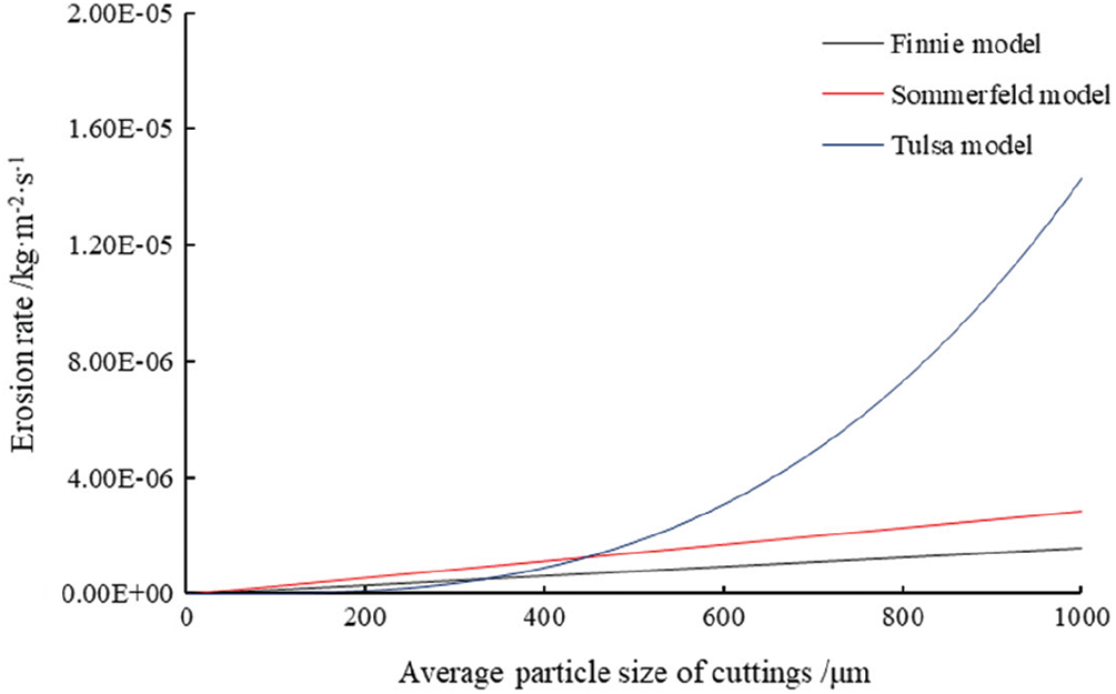
Figure 6: Influence of average particle size of cuttings on erosion rate
5.4 Influence of Cuttings Density on Erosion Rate
When the impact angle of cuttings was set at 18°, the impact velocity at the drill collar was 21.74 m/s with an average particle size of 0.26 mm. The Boolean hardness of the pipe string was 260. Fig. 7 shows the relationship curve between the erosion rate and the average particle size of cuttings. It can be seen that the erosion rate calculated by each model increases with the increase of the average particle size of cuttings. The results of the Sommerfeld model are larger than those of other models.
Figure 7: Influence of cutting density on erosion rate
5.5 Influence of Hardness of Pipe String on Erosion Rate
The impact angle of cuttings was set to be 18°, and the impact velocity was set to be 21.74 m/s at the drill collar. The average particle size was 0.26 mm and the density was 1500 kg/m3. The relationship between the erosion rate and the Boolean hardness of the pipe column is calculated and presented in Fig. 8. The Tulsa model shows the relationship between the erosion rate and Boolean hardness. The greater the hardness of the string, the smaller the erosion damage.
Figure 8: Influence of pipe string properties on erosion rate
5.6 Erosion Analysis of Field Pipe String
When analyzing the erosion of string in Well H and Well D, the impact angle was 18°, the density of cuttings was 1500 kg/m3, and the average particle size of cuttings was 0.26 mm. The drill collar Brinell hardness was 341, and the drill pipe Brinell hardness was 260. Column erosion. The pure drilling time of Well H was 8 h 35 min, and the mixed fluid flow rate at the drill collar was 67.98 m/s. The pure drilling time of Well D was 45 h 39 min, and the flow rate of mixed fluid at the drill collar was 21.74 m/s.
The three models of the gas drilling process on the string erosion calculation results are listed in Tables 8, 9, Figs. 9, and 10.


Figure 9: Erosion of well string in Well D
Figure 10: Erosion of well string in Well H
The Sommerfeld model and the Tulsa model show the relationship between the erosion of string and the particle size of cuttings in the two wells. In the pure drilling time, the residual wall thickness of Wells H and D is greater than 70%, which is lower than the erosion wear failure standard.
This paper calculates the minimum gas injection rate of nitrogen drilling in a coal seam with abundant rainwater in the study area, and analyzes the erosion of pipe string. The calculation results were compared with the field data. The following conclusions were reached.
1. The minimum gas injection rate of wells with water production in the formation calculated by the Guo model was 67.4 m3/min, which was 90–120 m3/min in actual use. The minimum gas injection rate of the well without water was 49.4 m3/min, and the actual use was 110 m3/min. The difference between the calculated injection pressure and the field value of wells with water in the formation was 6.5%–15.2%. The difference of no effluent was 0.65%–7.32%. The comparison between the calculation results and the field data shows that the Guo model can better calculate the situation of no water formation in the nitrogen drilling of the coal seam.
2. Cuttings density, particle size, impact velocity and angle, and string hardness have significant effects on the erosion rate. The Finnie model, Sommerfeld model, and Tulsa model have different sensitivities to these factors, so they need to be used at the same time to analyze the string erosion. The erosion damage of the pipe string at the wellhead is large, and the erosion damage of the pipe string in the field does not reach the failure standard.
Acknowledgement: The authors would like to extend their thanks to the learning and research platform, as well as the generous financial support provided by the company and the school.
Funding Statement: National Science and Technology Major Special Project, 2016ZX05044, CBM Development Technology and Pilot Test in East Yunnan and Western Guizhou.
Conflicts of Interest: The authors declare that they have no conflicts of interest to report regarding the present study.
1. Angel, R. (1957). Volume requirements for air or gas drilling. Transactions of the AIME, 210(1), 325–330. DOI 10.2118/873-G. [Google Scholar] [CrossRef]
2. Chen, X., Gao, D., Guo, B. (2014). A new method for determining the minimum gas injection rate required for hole cleaning in horizontal gas drilling. Journal of Natural Gas Science and Engineering, 21(4), 1084–1090. DOI 10.1016/j.jngse.2014.11.009. [Google Scholar] [CrossRef]
3. Sun, B., Xiang, C., Wang, Z. (2012). Influence of altitudes and air humidity to the minimum gas injection rate in air underbalanced drilling. Open Petroleum Engineering Journal, 5(1), 104–108. DOI 10.2174/1874834101205010104. [Google Scholar] [CrossRef]
4. Guo, B., Ghalambor, A., Siping, X. (2006). Calculation of gas volume flow in underbalanced drilling. China: Sinopec Press. [Google Scholar]
5. Tabatabaei, M., Ghalambor, A., Guo, B. (2008). The minimum required gas-injection rate for liquid removal in air/gas drilling. SPE Annual Technical Conference and Exhibition, SPE116135, Denver, Colorado, USA. [Google Scholar]
6. Yang, X. G., Liu, G. H., Li, J. (2015). Application of a special technique for controlling the cutting bed height in gas drilling of horizontal wells. Chemistry & Technology of Fuels & Oils, 50(6), 508–515. DOI 10.1007/s10553-015-0557-1. [Google Scholar] [CrossRef]
7. Wei, N., Meng, Y. F., Li, G., Li, Y. J., Liu, A. Q. et al. (2014). Cuttings-carried theory and erosion rule in gas drilling horizontal well. Thermal Science, 18(5), 1695–1698. DOI 10.2298/TSCI1405695W. [Google Scholar] [CrossRef]
8. Sun, B. J., Xiang, C. S., Wang, Z. Y. (2012). Influence of altitudes and air humidity to the minimum gas injection rate in air underbalanced drilling. Open Petroleum Engineering Journal, 5(1), 104–108. DOI 10.2174/1874834101205010104. [Google Scholar] [CrossRef]
9. Xu, R. Q. (2020). Simulation analysis of vertical gas well production string erosion model. Total Corrosion Control, 34(6), 58–62, 66. DOI 10.13726/j.cnki.11-2706/tq.2020.06.058.05. [Google Scholar] [CrossRef]
10. Taji, I., Hoseinpoor, M., Moayed, M. H. (2020). Pitting corrosion of 17-4ph stainless steel: Impingement of a fluid jet vs. erosion-corrosion in the presence of the solid particles. Journal of Bio- and Tribo-Corrosion, 6(4), 1–7. DOI 10.1007/s40735-020-00428-w. [Google Scholar] [CrossRef]
11. Liu, S. H., Zheng, H. L., Zhu, X. H. (2014). Drill string failure analysis and erosion wear study at key point for gas drilling. Energy Exploration & Exploitation, 32(3), 553–568. DOI 10.1260/0144-5987.32.3.553. [Google Scholar] [CrossRef]
12. Zhu, X. H., Liu, S. H., Tong, H., Huang, X., Li, J. (2012). Experimental and numerical study of drill pipe erosion wear in gas drilling. Engineering Failure Analysis, 26(9), 370–380. DOI 10.1016/j.engfailanal.2012.06.005. [Google Scholar] [CrossRef]
13. Nam, C. Y., Lee, Y. K., Park, G. H., Lee, G. H., Lee, W. O. (2018). Analysis of pipe failure period using pipe elbow erosion model by computational fluid dynamics (CFD). Korean Chemical Engineering Research, 56(1), 133–138. DOI 10.9713/kcer.2018.56.1.133. [Google Scholar] [CrossRef]
14. Huang, X., Liu, Q. (2012). An erosion model of drill string based on process parameters of gas drilling. Acta Petrolei Sinica, 33(5), 878–880. DOI 10.7623/syxb201205020. [Google Scholar] [CrossRef]
15. Vieira, R., Shirazi, S. (2021). A mechanistic model for predicting erosion in churn flow. Wear, (10), 203654. DOI 10.1016/j.wear.2021.203654. [Google Scholar] [CrossRef]
16. Zhang, X., Jia, Z. (2019). Influence of ground stress on coal seam gas pressure and gas content. Fluid Dynamics & Materials Processing, 15(1), 53–61. DOI 10.32604/fdmp.2019.04779. [Google Scholar] [CrossRef]
17. Yukie, M., Haruyuki, M., Kaname, M. (2018). Analysis of roadside air pollution in Osaka city using biomonitoring method. Journal of Japan Society for Atmospheric Environment, 53(3), 79–87. DOI 10.11298/taiki.53.79. [Google Scholar] [CrossRef]
18. National Petroleum Standardization Technical Committee (2004). Technical conditions for scrapping drilling tools. SY/T 5956-2004. China: China Standards Press. [Google Scholar]
19. National Petroleum Standardization Technical Committee (2012). Management and use of kelly. SY/T 5369-2012. China: China Standards Press. [Google Scholar]
20. Wang, Z., Luo, W., Liao, R., Xie, X., Han, F. et al. (2019). Slug flow characteristics in inclined and vertical channels. Fluid Dynamics & Materials Processing, 15(5), 583–595. DOI 10.32604/fdmp.2019.06847. [Google Scholar] [CrossRef]
21. Ba, Q. B., Liu, Y. B., Zhang, Z. G., Xiong, W., Shen, K. (2021). Analysis of the flow field characteristics associated with the dynamic rock breaking process induced by a multi-hole combined external rotary bit. Fluid Dynamics & Materials Processing, 17(4), 697–710. DOI 10.32604/fdmp.2021.014762. [Google Scholar] [CrossRef]
 | This work is licensed under a Creative Commons Attribution 4.0 International License, which permits unrestricted use, distribution, and reproduction in any medium, provided the original work is properly cited. |