| Fluid Dynamics & Materials Processing |
DOI: 10.32604/fdmp.2022.017899
ARTICLE
Free Convection of a Viscous Electrically Conducting Fluid Past a Stretching Surface
1Department of Mechanical Engineering, Faculty of Engineering, Albaha University, Al Bahah, 65527, Saudi Arabia
2Department of Mathematics, College of Engineering and Technology, Bhubaneswar, Odisha, 751029, India
3Department of Mathematics, Centurion University of Technology and Management, Bhubaneswar, Odisha, 751009, India
4Department of Mathematics, Siksha ‘O’ Anusandhan Deemed to be University, Bhubaneswar, Odisha, 751030, India
5Physics Department, College of Science, Al-Zulfi, Majmaah University, AL-Majmaah, 11952, Saudi Arabia
*Corresponding Author: Iskander Tlili. Email: l.tlili@mu.edu.sa
Received: 15 June 2021; Accepted: 12 August 2021
Abstract: Free convection of a viscous electrically conducting liquid past a vertical stretching surface is investigated in the presence of a transverse magnetic field. Natural convection is driven by both thermal and solutal buoyancy. The original partial differential equations governing the problem are turned into a set of ordinary differential equations through a similar variables transformation. This alternate set of equations is solved through a Differential Transform Method (DTM) and the Pade approximation. The response of the considered physical system to the non-dimensional parameters accounting for the relative importance of different effects is assessed considering different situations.
Keywords: Viscous fluid; magnetohydrodynamic (MHD); thermal and mass buoyancy; differential transform method and pade approximant
Nomenclature
| a | constant |
| T∞ | ambient temperature |
| B0 | magnetic field strength |
| u | velocity of the fluid along x-axis |
| C | fluid concentration |
| uw | characteristic velocity |
| Cf | non-dimensional skin friction |
| v | velocity of the fluid along y-axis |
| Cw | concentration of the plate |
| x, y | co-ordinate axes along and |
| C∞ | ambient concentration perpendicular to the plate |
| DB | molecular diffusivity |
| Greek Symbols | |
| f | dimensionless stream function |
| α | thermal diffusivity |
| f′ | dimensionless velocity profile |
| ν | kinematic viscosity |
| g | acceleration due to gravity |
| β1 | coefficient of thermal expansions |
| k | vortex viscosity |
| β2 | coefficient of solutal expansions |
| M | magnetic parameter |
| η | similarity variable |
| Nux | Nusselt number |
| θ | dimensionless temperature |
| | Prandtl number |
| ϕ | dimensionless concentration |
| qm | mass transfers from the plat |
| ψ | stream function |
| qw | heat transfers from the plat |
| μ | coefficient of viscosity |
| | Reynold number |
| σ | magnetic permeability of fluid |
| Sc | Schmidt number |
| ρ | fluid density |
| Shx | Sherwood number |
| λ1 | thermal buoyancy parameter |
| T | fluid temperature |
| λ2 | solutal buoyancy parameter |
| Tw | constant temperature of the plate |
| τw | the wall shear stress |
In recent the application of flow phenomena over a stretching surface is vital due to its uses in the production of materials in several industrial processes. However, these are composed with the heat and mass transfer phenomena and for the design of various equipment’s, the role of heat transfer is important. In particular, the production of plastic sheets, space vehicle aircrafts, gas turbines etc. the knowledge of radiating heat transfer is useful. To reveal the principle of buoyancy according to the engineering context its application is vast. The principle of buoyancy can be useful for the floating of the objects such as ships and boats, submarines, hydrometer, balloons and airships and many others. Further, in view of mathematics, the nonlinear equations are supreme factors for the studies relating to it. Many nonlinear equations don’t have an accurate analytic technique to solve for which numerical methods have been employed. There are some analytic methods like Adomian Decomposition Method (ADM), Differential Transform Method (DTM), Variation of Parameters Method (VPM), Perturbation method and Homotopy Perturbation Method (HPM) that can be employed to solve nonlinear equations easily.
Considering the free convection of air past a vertical plate in presence of earth’s gravitational field is one of the above cases was analyzed by Schmidt et al. [1]. Mishra et al. [2] have presented heat and mass transfer analysis over Walters’ B’model over an extended surface. For the solution of the flow problem they have employed Kummer’s function, an analytical technique. Especially, they have investigated the heat equation for two cases such as PST and PWHF. Earlier Mishra et al. [3] have proposed a work to investigate the flow of an incompressible fluid on a vertical flat plate where they have used numerical technique to solve the problem. Another detailed study on the viscous incompressible fluid over a vertical flat plate was encountered by Pattnaik et al. [4] where they have employed Laplace transform technique of both time-dependent and independent cases since, Laplace transform technique is an effective technique for some coupled equations. Pattnaik et al. [5,6] have considered this technique to analyze an unsteady MHD flow to study the angle of inclination on the flow circumstances.
For the current study, the collection is obtained for some special literature review [7–10] regarding DTM transformations and its applications for electric circuits, especially how it works on heat transfer equation, solution for a system of second and higher-order equations. Recently, Sepasgozara et al. [11] have looked forward in their work for a non-Newtonian viscoelastic fluid flow employing DTM and here authors have compared the result with numerical technique also and both results obey with good accuracy. Jena et al. [12–15] found some more related studies on Jeffery fluid flow, viscoelastic fluid flow, and micropolar nanofluid flow where authors have used different methods such as numerical technique, Kummer’s function and ADM technique for the solution of non-dimensional governing equations.
There is an investigation by Usman et al. [16] for DTM and Runge-Kutta of order four which describes that DTM is a much more effective technique to solve and this kind of results can help researchers for quicker and easier analysis. For the first time the great mathematician Baker had written a book namely Essentials of Pade Approximants and our research work is comprehensively occupied by his study [17]. Through in this book, the author has given a very clear and elaborate description of Pade Approximants, solution for Pade Approximants, the Pade table, and the structure of the Pade table, etc. Another four-step Pade algorithm is used to solve ODEs and that has been carried out by Boyd [18]. The author has mentioned all the four steps starting from series expansion to multiple solutions of equations. For the reduction of fuel consumption, a non-uniform slab heating pattern in a furnace is used by Ajili et al. [19]. Discreet ordinates thermal radiation is eployed to carry out the load distribution effect. Dehkordi et al. [20] considered the Fe3O4-water nanofluid for the influence of electric field in a microchannel and its major application is used in boiling processes. The investigation was carried out as a study of molecular dynamics. Further, the development in the said work is obtained by simulating the thermal domains considering Cu-water nanofluid in a nanochannel that is proposed by Asgari et al. [21]. Karimipour and his co-workers [22] have analyzed the behavior on the physical properties of thermal conductivity in a byhrid nanofluid composed of Cu and CNT nanopartcles. Cattaneo-Christov heat flux model is proposed by Nadeem et al. [23–25] in various non-Newtonian fluid considering different geometries. Muhammad et al. [26,27] and Nadeem et al. [28,29] conducted the work on the ferromagnetic fluid for the influence of various thermal properties with stratification condition. Rashidi et al. [30] have investigated the mixed convection problem about a flat plate embedded in a porous medium by implementing DTM along with the Pade approximation technique. Further, the study is compared with a numerical investigation to enhance the quality of research and for the accuracy check. In another study also Rashidi et al. [31] studied the flow pattern of the MHD flow using a combination of both DTM and Pade approximation method. Here authors have compared DTM with DTM-Pade and both these with Runge-Kutta fourth-order method. Also through this study authors concluded that DTM-Pade is an excellent and quicker method to solve boundary value problems. Authors in different works [32–36] have shown their interest in MHD flow using the DTM-Pade technique as the prior investigation on different fluid flow problems. The performance of the radiative heat on the melting heat transport phenomenon for the flow using nanomaterials with irreversibility analysis is conducted by Khan et al. [37]. Further, Hayat et al. [38] presented the irreversibility characteristics in the flow of nanofluids with the interaction of velocity slip and dissipative heat energy by a stretchable cylinder. Hayat and his co-workers [39–44] have presented the simulation and modeling of entropy optimization for various nanoliquids considering different geometries.
With reference to the aforesaid discussions, the aim of the present investigation is to reveal the impact of buoyancy forces on the two-dimensional flow of conducting viscous fluid past an expanding surface. The present study overrides the earlier investigation by imposing an approximate analytical technique called Differential Transform Method and along with the enhanced solution is obtained by employing Pade approximant. The comparison also obtained and presented graphically.
A steady two-dimensional flow of viscous fluid over a vertical stretching surface is undertaken in the present investigation. The flow occurs in the direction of x-axis and y-axis is transverse to it. The fluid becomes electrically conducting due to the applied magnetic field of strength B0 is acted along the flow direction i.e., normal to y-axis. The surface temperature and concentration are deployed as Tw and Cw respectively. Similarly, the ambient conditions are also presented in Fig. 1.
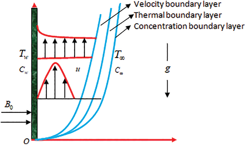
Figure 1: Flow geometry
Assuming the aforesaid conditions and following [32] the governing flow phenomena are presented as
where
The corresponding boundary conditions are expressed as follows:
To transformed into the non-dimensional form the followings [45] are the suitable and defined as
Using the aforesaid equations, Eq. (1) is identically satisfied and Eqs. (2)–(4) become
where
Besides, the converted boundary conditions are prescribed as follows:
The physical quantities for the said problem are as follows:
Applying the non-dimensional transformations (7) we have
where
Based upon the Taylor series expansion the methodology i.e., differential transform method, a semi-analytical method, is illustrated here. To get a series solution in terms of polynomials the differential equations are converted into a set of recurrence relations. Zhou [7] first proposed the concept of differential transform to electric circuit problems.
The transformation of kth derivative of the defined function f(x) is
The inverse transform of F(k) is defined as
Substituting F(k) from Eq. (14) in Eq. (15) we get
This is Taylor’s series expansion of f(x) about x = x0.
The method provide solutions in terms of convergent series with easily computable components. The aim of this article is to introduce the DTM as an efficient tools to solve the highly nonlinear differential equations. We choose a similarity transform variable to modify Navier–Stokes equation to a coupled highly non-linear ordinary differential equation which then solved by using DTM along with Pade technique to get close form solution. To illustrate the simplicity and accuracy of its variants by comparing the results with numerical solution by using bvp5c technique, a MATLAB solver. This work introduces the DTM for two reasons:
(i) This method gives a good sense of continuation to the Taylor series in the application of differentiation.
(ii) This method is gaining momentum among researchers due to its simplicity and has some pedagogical benefits.
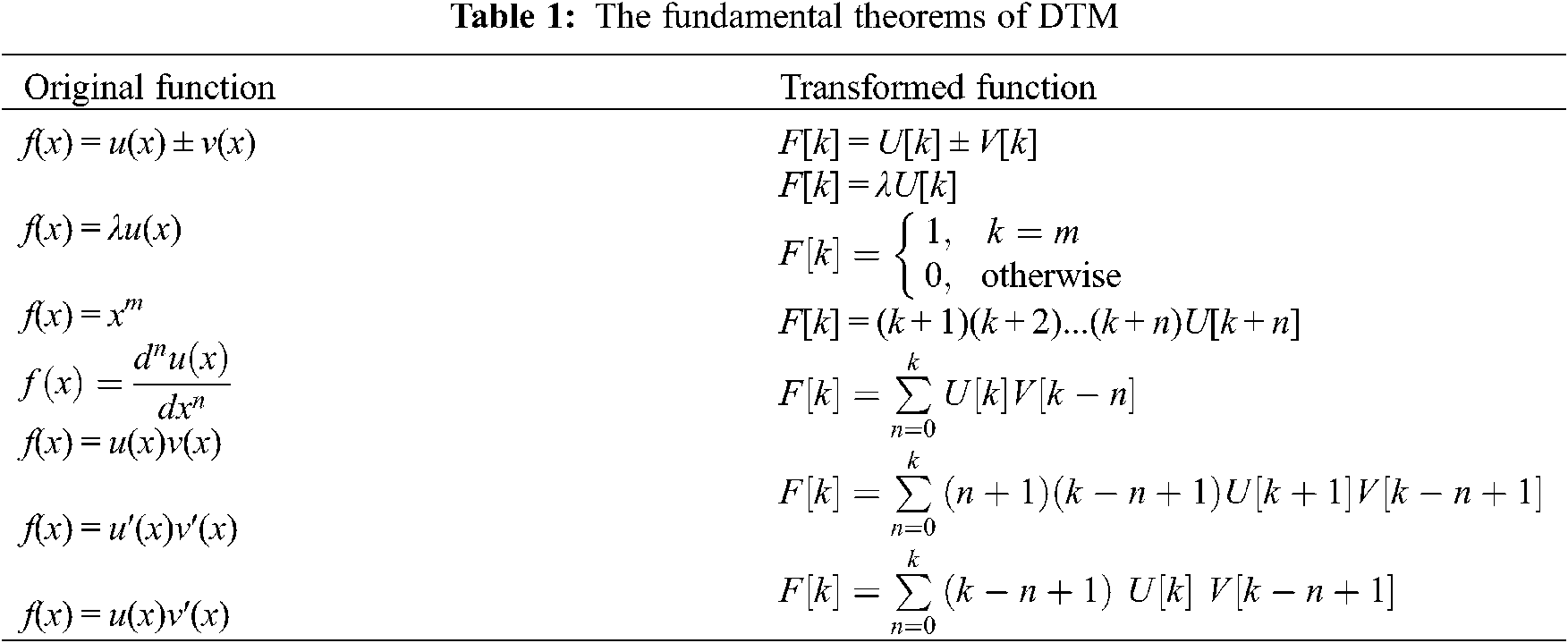
This method constructs an analytical solution of linear as well as non-linear differential equations in the form of a polynomial. Though it uses the general form of the traditional high-order Taylor series method, it overcomes the inefficient sides of Taylor series method which takes a long time for higher orders. Symbolic computations of the necessary derivatives of the data functions are computed by using iterative procedure for obtaining analytical solutions of differential equations. From Eqs. (14) and (15), the fundamental theorems of DTM can be deduced, which are listed in Table 1.
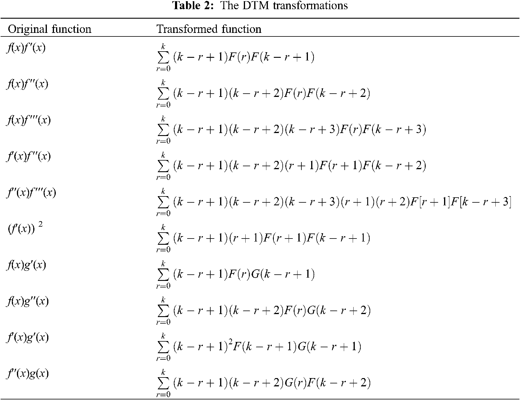
The DTM transformations which we used in the present work are listed in Table 2.
Taking the differential transforms of Eqs. (8)–(10), we obtained Eqs. (17)–(19), respectively
where F(k), Θ (k) and Φ(k) are the differential transforms of f(t), θ(t) and ϕ(t) respectively. The boundary conditions Eq. (11) are transformed as
Solving Eqs. (17)–(19) with Eq. (20) we derived the DTM solutions as
To proceed with our work we have taken
After applying DTM to get an accurate solution of the boundary value problem, we have applied Pade Approximant.
The Pade approximant of f(η) on [a, b] is a rational fraction of two polynomials PN(η) and QM(η), where degrees N and M are degree of the polynomials, respectively [17].
The power series form of the function f(η) is
The notation ci, i = 0, 1, 2, ... is reserved for the given set of coefficients and f(η) is the associated function. [L/M] Pade approximant is a rational fraction.
which has a Maclaurin expansion, agrees with Eq. (27). It is noticed that in Eq. (28) there are L + M + 1 unknown coefficient in all. This number suggests that normally [L/M] ought to fit the power series Eq. (27) through the orders 1, η, η2,... , ηL+M. In the notation of formal power series
Equating the coefficients of ηL+1, ηL+2, ... , ηL+M we get
If i < 0, we define ci = 0 for consistency. Since b0 = 1, Eq. (30) becomes a set of M linear equations for M unknown denominator coefficients.
From the above expression, bi may be obtained. The numerator coefficients a0, a1,…….aL follow immediately from Eq. (29) by equating the coefficients of 1, η, η2,... , ηL+M such as
Thus, Eqs. (29) and (32) normally determine the Pade approximants.
Pade approximant is used to bring the infinite boundary layer behaviour of the solution obtained by DTM. The Pade approximant gives a better closed form solution when applied after DTM, and it may still work where the DTM as well as Taylor series does not converge. For these reasons we have used Pade approximants. Since Pade approximant is a rational function, it can be used to get the initial values of the function of higher order which may contain an artificial singular point, but this can be avoided.
Following, we have calculated diagonal Pade approximant of order [2/2] of f′(η), θ(η) and ϕ(η) as
where
We get,
So, the desired solutions of Eqs. (24)–(26) are becomes
An electrically conducting viscous liquid past a vertical stretching surface via the influences of thermal ad buoyancy is characterized in the present analysis. As a novelty of the investigation, we aim to solve the transformed differential equations using the Differential transform method, and the refinement of the solution is obtained by Pade approximant. Finally, the numerical results are compared with the earlier investigation carried out by the help of the numerical method. The variation of the physical quantities affecting the flow phenomena is presented via graphs and the physical significance of each parameter is deployed. At the time of computation the variation of parameters in the corresponding figure is displayed for the fixed values of other pertinent parameters laid down as;
The present section displays the validation graphs of transverse and longitudinal velocities, energy, and solutal profiles using the current methodology and the earlier numerical method via Figs. 2–6.
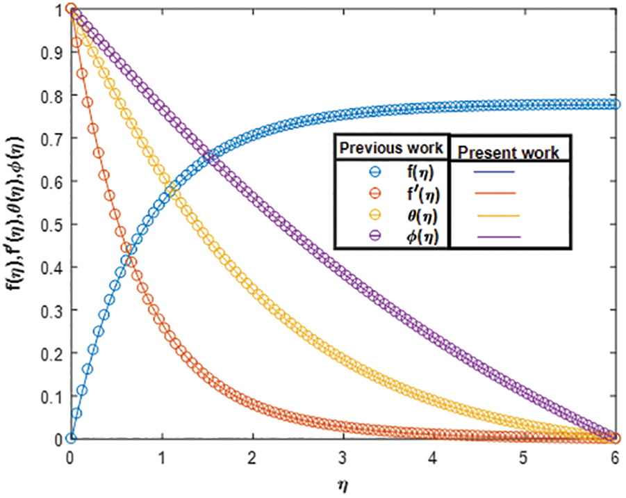
Figure 2: Validation profile with the previous study
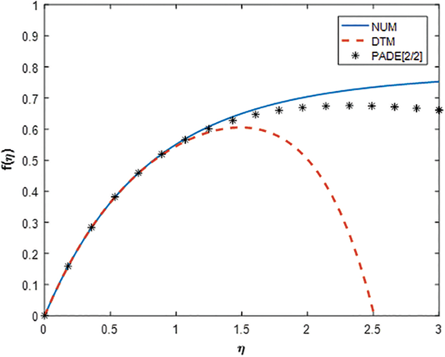
Figure 3: Comparison of stream function
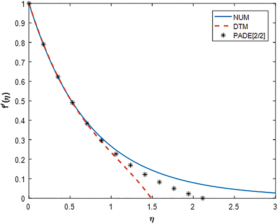
Figure 4: Comparison of velocity profile
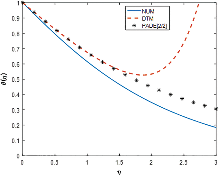
Figure 5: Comparison of temperature profile
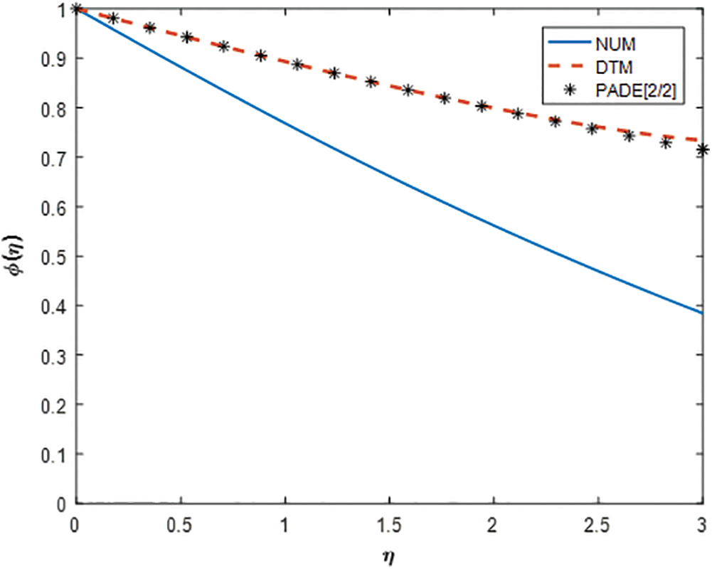
Figure 6: Comparison of concentration profile
In Fig. 2, the coincide results of all the profiles with the work of Ajili et al. [19] in a particular case (M = 0, λ1 = 0, λ2 = 0). This result shows the convergence criteria of the methodology applied in the present study and also shows a road map for further investigation using several values of different physical parameters.
Fig. 3 illustrates the comparison of transverse velocity profile solved earlier using numerical methods with that of present DTM and its refinement Pade approximant. From the figure, it is noteworthy that, the better approximate result by the Pade approximant method of the corresponding DTM coincides with the earlier numerical method up to a great extent. All the profiles are coincident to each other within a certain region and afterward, deviation occurs. This phenomenon depends upon the order of the DTM applied herewith. In the present case, the [2/2] order Pade approximant is used. Higher-order approximation may result in more accurate results for various contributing parameters.
Fig. 4 portrays the similar behavior of the profiles on the longitudinal velocity distribution. As a concluding remark, it reveals that the methodologies applied in the present paper have a greater convergence rate depending upon the order of preference. However, the higher-order Pade, the rational approximation will give better accuracy for all the profiles.
The comparison plots for the fluid temperature and concentration in all these methods are displayed via Figs. 5 and 6 respectively. Although the resulting analysis is similar to that of an earlier description so it is not wise to repeat.
The computational behavior of the physical parameters, i.e., magnetic parameter, Prandtl number, thermal, and mass buoyancy parameters are exhibited in Fig. 7. Fig. 7a deployed the characteristics of the magnetic parameter on the longitudinal velocity distribution for the several values of other pertinent parameters. The inclusion of the magnetic field contributed by the resistive force offered by the Lorentz force retards the velocity profile significantly for which the velocity boundary layer thickness also retards. The resistive force opposes the profile to boost up. The variation of the Prandtl number on the velocity distribution is illustrated in Fig. 7b. The higher Prandtl number diminishes the velocity profile asymptotically to meet the requisite boundary conditions. Sudden fall near the surface of the sheet is marked within the domain η < 2 and further, the profile becomes smooth. However, increasing rate the of the boundary layer thickness of the velocity profile retards significantly. Figs. 7c and 7d elucidate the buoyancy effects offered by both the thermal and mass buoyancy parameters on the velocity distribution. It is seen that enhancement in the profile occurs due to the increase in the buoyancy parameter. The overshot in the profiles is due to the buoyancy parameters.
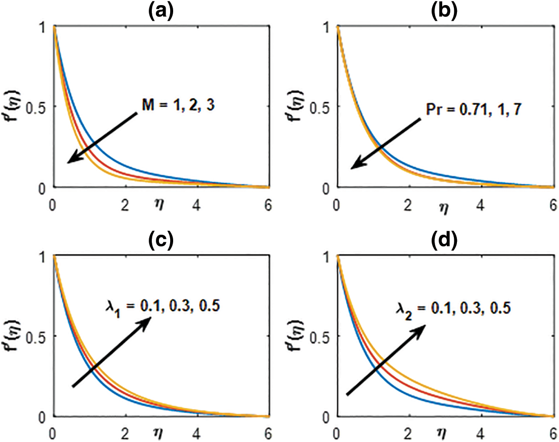
Figure 7: Velocity distribution profile for (a)
The efficiency of the physical parameters such as magnetic parameter, Prandtl number, thermal, and mass buoyancy on the fluid temperature is displayed via Fig. 8. The distribution of the magnetic parameter on the temperature is shown in Fig. 8a. It is observed that an increase in the magnetic parameter boosts up the temperature profile. The fact is the magnetic parameter that retards the velocity profiles, the stored energy overshoots the fluid temperature. Fig. 8b presents the behavior of the Prandtl number on the fluid temperature. Prandtl number is the ratio of kinematic viscosity with that of thermal diffusivity. An increase in Prandtl number means the thermal diffusivity decreases resulted in the temperature decreases. Figs. 8c and 8d exhibit the buoyancy effects on the fluid temperature with the fixed values of other pertinent parameters. Increasing buoyancy retards the fluid temperature in the entire domain.
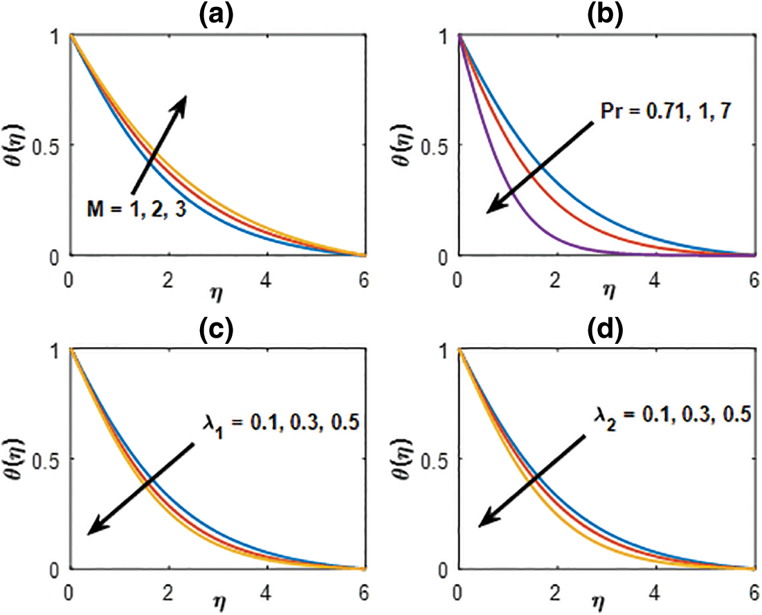
Figure 8: Temperature distribution profile for (a)
4.4 Concentration Distribution
Fig. 9 illustrates the variation of the magnetic parameter, Schmidt number, and both the thermal and mass buoyancy parameters on the fluid concentration. It is clear from Fig. 9a that, the increasing magnetic parameter enhances the fluid concentration. The role of the heavier density characterized by the Schmidt number is described in Fig. 9b. In the present case, we have considered the Hydrogen (H), Helium (He) and Ammonia (NH3) with their corresponding values of Sc presented in the figure. It is seen that the heavier density parameter retards the concentration of the fluid significantly. Similar observations are marked in Figs. 9c and 9d for the behavior of the buoyancy parameters on the concentration profiles.
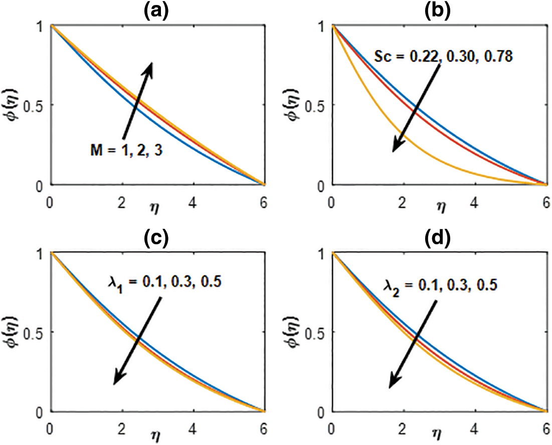
Figure 9: Concentration distribution profile for (a) M, (b) Sc, (c) λ1 and (d) λ2
4.5 Physical Quantities of Interest
The computation of the physical quantities of interest, i.e., the coefficients of shear stress, rate of heat, and mass transfer for several values of contributing parameters are described in Figs. 10–12. The coefficient of shear stress for the variation of buoyancy parameters and the Prandtl number vs. magnetic parameter is displayed in Figs. 10a and 10b. The shear rate enhances with the increased thermal and mass buoyancy parameter whereas in comparison to both the parameters it is observed that the mass buoyancy overrides the efficiency of the thermal buoyancy parameter. However, the reverse impact is observed for the increasing Prandtl number with the variation of the magnetic parameter.
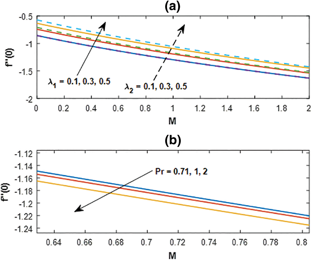
Figure 10: Skin friction profile for (a) λ1, λ2 and (b)
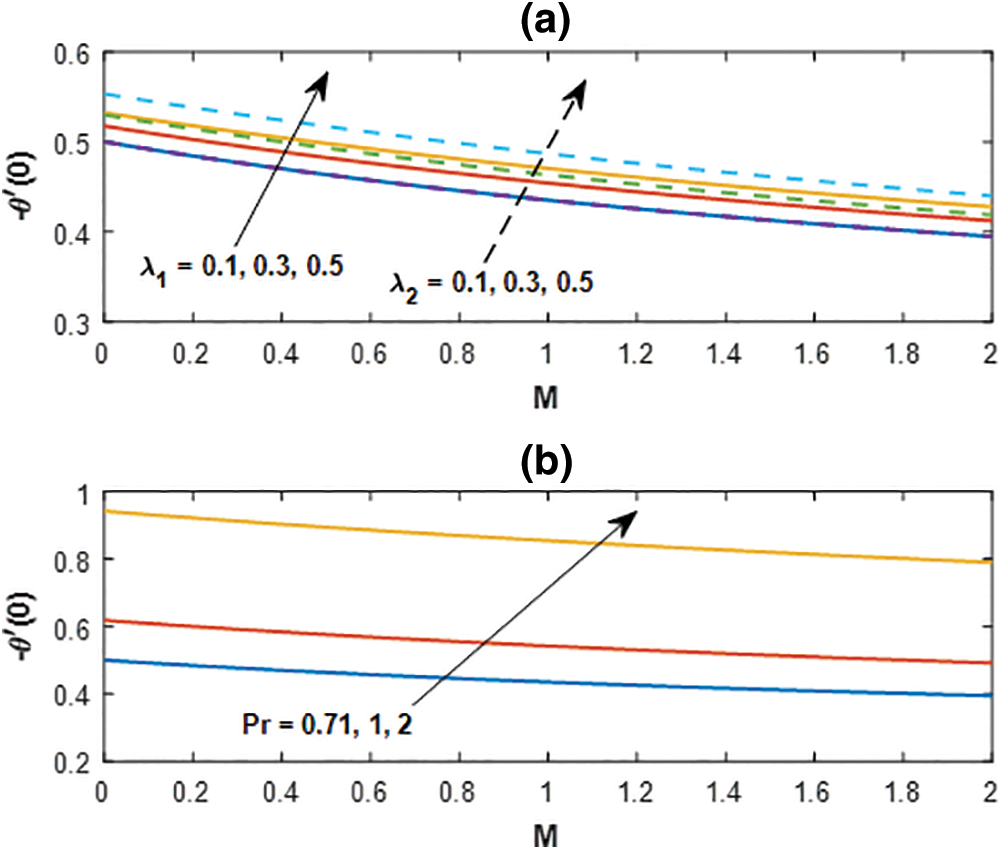
Figure 11: Nusselt number profile for (a) λ1, λ2 and (b)
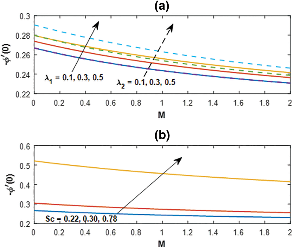
Figure 12: Sherwood number profile for (a) λ1, λ2 and (b) Sc with M
Fig. 11a represents the influences of buoyant forces and Fig. 11b deployed with the variation of Prandtl number on the rate of heat transfer coefficients. An increase in Prandtl number favors in to enhance the rate of heat transfer.
The behavior of thermal and mass buoyancy parameters on the rate of mass transfer is presented in Fig. 12a and the variation of Schmidt number is displayed in Fig. 12b versus the magnetic parameter. An increase in buoyant forces boosts up the concentration rate with the increasing magnetic parameter throughout and the heavier species also enhances the rate significantly.
The approximate analytical approach for the study of the steady two-dimensional flow of viscous fluid in the presence of the magnetic field is analyzed in the present investigation. The transformed governing equations are tackled by using the Differential transform method and its refinement using the Pade approximant method for the various values of contributing parameters. The validation with the earlier numerical method was also established. However, the conclusive remarks for various physical parameters described earlier are presented below.
The validation with earlier study presents road map for the further investigation on the physical properties of contributing parameters.
• The Pade approximant shows a better accuracy than that of the numerical as well as the DTM applied for the said problem.
• Heavier viscous diffusivity produces higher Prandtl number retards the velocity distribution at all points within the flow domain.
• Buoyant driven forces enhances the velocity distributions whereas impact is opposite in the case of temperature distributions.
• Mass buoyancy parameter is counterproductive than that of thermal buoyancy for the enhancement in the shear rate coefficient.
• Heavier species favours is to boost up the rate of mass transfer with increasing magnetic parameter.
Acknowledgement: We are very much thankful to learned reviewers for their useful suggestions for the improvement in the quality of our manuscript.
Funding Statement: The authors received no specific funding for this study.
Conflicts of Interest: The authors declare that they have no conflicts of interest to report regarding the present study.
1. Schmidt, E., Beckmann, W. (1930). Das Temperatur-und Geschwindigkeitsfeld vor einer Wärme abgebenden senkrechter Platte bei natürlicher Konvektion. Technische Mechanik und Thermodynamik, 1, 391–406. [Google Scholar]
2. Mishra, S. R., Pattnaik, P. K., Bhatti, M. M., Abbas, T. (2017). Analysis of heat and mass transfer with MHD and chemical reaction effects on viscoelastic fluid over a stretching sheet. Indian Journal of Physics, 91(10), 1219–1227. DOI 10.1007/s12648-017-1022-2. [Google Scholar] [CrossRef]
3. Mishra, S. R., Pattnaik, P. K., Dash, G. C. (2015). Effect of heat source and double stratification on MHD free convection in a micropolar fluid. Alexandria Engineering Journal, 54, 681–689. DOI 10.1016/j.aej.2015.04.010. [Google Scholar] [CrossRef]
4. Pattnaik, P. K., Biswal, T. (2015). Analytical solution of MHD free convective flow through porous media with time dependent temperature and concentration. Walailak Journal of Science & Technology, 12(9), 749–762. DOI 10.14456/1130. [Google Scholar] [CrossRef]
5. Pattnaik, J. R., Dash, G. C., Singh, S. (2012). Radiation and mass transfer effects on MHD free convection flow through porous medium past an exponentially accelerated vertical plate with variable temperature. Annals of faculty engineering hunedoara. International Journal of Engineering, Tome X(3), 175–182. [Google Scholar]
6. Pattnaik, J. R., Dash, G. C., Singh, S. (2017). Radiation and mass transfer effects on MHD flow through porous medium past an exponentially accelerated inclined plate with variable temperature. Ain Shams Engineering Journal, 8, 67–75. DOI 10.1016/j.asej.2015.08.014. [Google Scholar] [CrossRef]
7. Zhou, J. K. (1986). Differential transformation and its applications for electrical circuits. Huazhong University Press, Wuhan, China. [Google Scholar]
8. Ayaz, F. (2004). Solutions of the systems of differential equations by differential transform method. Applied Mathematics and Computation, 147(2), 547–567. DOI 10.1016/S0096-3003(02)00794-4. [Google Scholar] [CrossRef]
9. Kurnaz, A., Oturanc, G. (2005). The differential transform approximation for system of ordinary differential equations. International Journal of Computer Mathematics, 82, 709–719. DOI 10.1080/00207160512331329050. [Google Scholar] [CrossRef]
10. Yaghoobi, H., Torabi, M. (2011). The application of differential transformation method to nonlinear equations arising in heat transfer. International Communication of Heat and Mass Transfer, 38, 815–820. DOI 10.1016/j.icheatmasstransfer.2011.03.025. [Google Scholar] [CrossRef]
11. Sepasgozara, S., Farajib, M., Valipourc, P. (2017). Application of differential transformation method (DTM) for heat and mass transfer in a porous channel. Propulsion and Power Research, 6(1), 41–48. DOI 10.1016/j.jppr.2017.01.001. [Google Scholar] [CrossRef]
12. Mishra, S. R., Jena, S.(2014). Numerical solution of boundary layer MHD flow with viscous dissipation. The Scientific World Journal, 2014, 5. DOI 10.1155/2014/756498. [Google Scholar] [CrossRef]
13. Jena, S., Mishra, S. R., Dash, G. C. (2017). Chemical reaction effect on MHD jeffery fluid flow over a stretching sheet through porous media with heat generation/absorption. International Journal of Applied & Computational Mathematics, 3, 1225–1238. DOI 10.1007/s40819-016-0173-8. [Google Scholar] [CrossRef]
14. Jena, S., Dash, G. C., Mishra, S. R. (2018). Chemical reaction effect on MHD viscoelastic fluid flow over a vertical stretching sheet with heat source/sink. Ain Shams Engineering Journal, 9, 1205–1213. DOI 10.1016/j.asej.2016.06.014. [Google Scholar] [CrossRef]
15. Mohapatra, D. K., Mishra, S. R., Jena, S. (2019). Cu-water and Cu-kerosene micropolar nanofluid flow over a permeable stretching sheet. Heat Transfer—Asian Research, 48, 2478–2496. DOI 10.1002/htj.21505. [Google Scholar] [CrossRef]
16. Usman, M., Hamid, M., Khan, U., Din, S. T. M., Iqbal, M. A. et al. (2018). Differential transform method for unsteady nanofluid flow and heat transfer. Alexandria Engineering Journal, 57, 1867–1875. DOI 10.1016/j.aej.2017.03.052. [Google Scholar] [CrossRef]
17. Baker, G. A. (1975). Essentials of pade approximants. London: Academic Press. [Google Scholar]
18. Boyd, J. (1997). Pade approximant algorithm for solving nonlinear ordinary differential equations boundary value problems on an unbounded domain. Computers in Physics, 11(3), 299–303. DOI 10.1063/1.168606. [Google Scholar] [CrossRef]
19. Ajili, S. H., Haratian, M., Karimipour, A., Bach, Q. Vu. (2020). Non-uniform slab heating pattern in a preheating furnace to reduce fuel consumption: Burners load distribution effects through semitransparent medium via discreet ordinates thermal radiation and k–ε turbulent model. International Journal of Thermophysics, 41(9), 128. DOI 10.1007/s10765-020-02701-z. [Google Scholar] [CrossRef]
20. Dehkordi, K. G., Karimipour, A., Afrand, M., Toghraie, D., Isfahani, A. H. M. (2020). The electric field and microchannel type effects on H2O/Fe3O4 nanofluid boiling process: Molecular dynamics study. International Journal of Thermophysics, 41(9), 132. DOI 10.1007/s10765-020-02714-8. [Google Scholar] [CrossRef]
21. Asgari, A., Nguyen, Q., Karimipour, A., Bach, Q. Vu., Hekmatifar, M. et al. (2020). Develop molecular dynamics method to simulate the flow and thermal domains of H2O/Cu nanofluid in a nanochannel affected by an external electric field. International Journal of Thermophysics, 41(9), 126. DOI 10.1007/s10765-020-02708-6. [Google Scholar] [CrossRef]
22. Karimipour, A., Malekahmadi, O., Karimipour, A., Shahgholi, M., Li, Z. (2020). Thermal conductivity enhancement via synthesis produces a new hybrid mixture composed of copper oxide and multi-walled carbon nanotube dispersed in water: Experimental characterization and artificial neural network modeling. International Journal of Thermophysics, 41(8), 116. DOI 10.1007/s10765-020-02702-y. [Google Scholar] [CrossRef]
23. Nadeem, S., Muhammad, N. (2016). Impact of stratification and Cattaneo-Christov heat flux in the flow saturated with porous medium. Journal of Molecular Liquids, 224, 423–430. DOI 10.1016/j.molliq.2016.10.006. [Google Scholar] [CrossRef]
24. Nadeem, S., Muhammad, N., Mustafa, T. (2017). Squeezed flow of a nanofluid with Cattaneo–Christov heat and mass fluxes. Results in Physics, 7, 862–869. DOI 10.1016/j.rinp.2016.12.028. [Google Scholar] [CrossRef]
25. Nadeem, S., Ahmad, S., Muhammad, N. (2017). Cattaneo-Christov flux in the flow of a viscoelastic fluid in the presence of Newtonian heating. Journal of Molecular Liquids, 237, 180–184. DOI 10.1016/j.molliq.2017.04.080. [Google Scholar] [CrossRef]
26. Muhammad, N., Nadeem, S., Haq, R. U. (2017). Heat transport phenomenon in the ferromagnetic fluid over a stretching sheet with thermal stratification. Results in Physics, 7, 854–861. DOI 10.1016/j.rinp.2016.12.027. [Google Scholar] [CrossRef]
27. Muhammad, N., Nadeem, S. (2017). Ferrite nanoparticles Ni-ZnFe2O4, Mn- ZnFe2O4, Mn-ZnFe2O4 and Fe2O4 in the flow of ferromagnetic nanofluid. The European Physical Journal Plus, 132(9), 377. DOI 10.1140/epjp/i2017-11650-2. [Google Scholar] [CrossRef]
28. Nadeem, S., Ahmad, S., Muhammad, N. (2018). Computational study of Falkner-Skan problem for a static and moving wedge. Sensors and Actuators B: Chemical, 263, 69–76. DOI 10.1016/j.snb.2018.02.039. [Google Scholar] [CrossRef]
29. Nadeem, S., Raishad, I., Muhammad, N., Mustafa, M. T. (2017). Mathematical analysis of ferromagnetic fluid embedded in a porous medium. Results in Physics, 7, 2361–2368. DOI 10.1016/j.rinp.2017.06.007. [Google Scholar] [CrossRef]
30. Rashidi, M. M., Laraqi, N., Sadri, S. M. (2010). A novel analytical solution of mixed convection about an inclined flat plate embedded in a porous medium using the DTM-padé. International Journal of Thermal Sciences, 49(12), 2405–2412. DOI 10.1016/j.ijthermalsci.2010.07.005. [Google Scholar] [CrossRef]
31. Rashidi, M. M., Keimanesh, M. (2010). Using differential transform method and padé approximant for solving MHD flow in a laminar liquid film from a horizontal stretching surface. Mathematical Problems in Engineering, 2010, 1–14. DOI 10.1155/2010/491319. [Google Scholar] [CrossRef]
32. Azimi, M., Ganji, D. D., Abbassi, F. (2012). Study on MHD viscous flow over a stretching sheet using DTM-pade’ technique. Modern Mechanical Engineering, 2, 126–129. DOI 10.4236/mme.2012.24016. [Google Scholar] [CrossRef]
33. Peker, H. A., Karaoglu, O., Oturanc, G. (2011). The differential transformation method and pade approximant for a form of classical Blasius equation. Mathematics and Computer Applications, 16(2), 507–513. DOI 10.3390/mca16020507. [Google Scholar] [CrossRef]
34. Thiagarajan, M., Senthilkumar, K. (2013). DTM-pade approximants for MHD flow with suction/blowing. Journal of Applied Fluid Mechanics, 6(4), 537–543. [Google Scholar]
35. Baag, S., Acharya, M. R., Dash, G. C. (2014). MHD flow analysis using DTM-pade and numerical methods. American Journal of Fluid Dynamics, 4(1), 6–15. DOI 10.5923/j.ajfd.20140401.02. [Google Scholar] [CrossRef]
36. Pattnaik, J. R., Dash, G. C., Ojha, K. L. (2017). MHD Falkner-Skan flow through porous medium over permeable surface. Modelling, Measurement and Control B, 86(2), 380–395. DOI 10.18280/mmc_b. [Google Scholar] [CrossRef]
37. Khan, S. A., Hayat, T., Alsaedi, A., Ahmad, B. (2021). Melting heat transportation in radiative flow of nanomaterials with irreversibility analysis. Renewable and Sustainable Energy Reviews, 140, 110739. DOI 10.1016/j.rser.2021.110739. [Google Scholar] [CrossRef]
38. Hayat, T., Khan, S. A., Alsaedi, A. (2021). Irreversibility characterization in nanoliquid flow with velocity slip and dissipation by a stretchable cylinder. Alexandria Engineering Journal, 60(3), 2835–2844. DOI 10.1016/j.aej.2021.01.018. [Google Scholar] [CrossRef]
39. Khan, S. A., Hayat, T., Alsaedi, A. (2020). Entropy optimization in passive and active flow of liquid hydrogen based nanoliquid transport by a curved stretching sheet. International Communications in Heat and Mass Transfer, 119, 104890. DOI 10.1016/j.icheatmasstransfer.2020.104890. [Google Scholar] [CrossRef]
40. Hayat, T., Khan, S. A., Alsaedi, A., ZaighamZai, Q. M. (2020). Computational analysis of heat transfer in mixed convective flow of CNTs with entropy optimization by a curved stretching sheet. International Communications in Heat and Mass Transfer, 118, 104881. DOI 10.1016/j.icheatmasstransfer.2020.104881. [Google Scholar] [CrossRef]
41. Khan, S. A., Hayat, T., Khan, M. I., Alsaedi, A. (2020). Salient features of Dufour and Soret effect in radiative MHD flow of viscous fluid by a rotating cone with entropy generation. International Journal of Hydrogen Energy, 45(28), 14552–14564. DOI 10.1016/j.ijhydene.2020.03.123. [Google Scholar] [CrossRef]
42. Khan, S. A., Saeed, T., Khan, M. I., Hayat, T., Khan, M. I. et al. (2019). Entropy optimized CNTs based Darcy-Forchheimer nanomaterial flow between two stretchable rotating disks. International Journal of Hydrogen Energy, 44(59), 31579–31592. DOI 10.1016/j.ijhydene.2019.10.053. [Google Scholar] [CrossRef]
43. Hayat, T., Khan, S. A., Khan, M. I. (2019). Theoretical investigation of Ree–Eyring nanofluid flow with entropy optimization and arrhenius activation energy between two rotating disks. Computer Methods and Programs in Biomedicine, 177, 57–68. DOI 10.1016/j.cmpb.2019.05.012. [Google Scholar] [CrossRef]
44. Hayat, T., Khan, S. A., Alwesaedi, A. (2020). Simulation and modeling of entropy optimized MHD flow of second grade fluid with dissipation effect. Journal of Materials Research and Technology, 9(5), 11993–12006. DOI 10.1016/j.jmrt.2020.07.067. [Google Scholar] [CrossRef]
45. Abo-Eldahab, E. M., El-Kady, M. M., Hallool, A. A. (2011). Effects of heat and mass transfer on MHD flow over a vertical stretching surface with free convection and joule heating. International Journal of Applied Maths & Physics, 3(2), 249–258. [Google Scholar]
 | This work is licensed under a Creative Commons Attribution 4.0 International License, which permits unrestricted use, distribution, and reproduction in any medium, provided the original work is properly cited. |