Fluid Dynamics & Materials Processing

DOI: 10.32604/fdmp.2022.017734

ARTICLE

CFD Analysis of Fluid-Dynamic and Heat Transfer Effects Generated by a Fixed Electricity Transmission Line Interacting with an External Wind

Yajuan Jia1, Lisha Shang1, Jiangping Nan1, Guangping Hu2 and Zhigang Fang3,4,*

1Xi’an Traffic Engineering Institute, Xi’an, China
2Xi’an Yuanai Electronic Technology Co., Ltd., Xi’an, China
3School of Automotive Engineering, Wuhan University of Technology, Wuhan, China
4Hubei Key Laboratory of Advanced Technology of Automotive Components, Wuhan University of Technology, Wuhan, China
*Corresponding Author: Zhigang Fang. Email: zhigang_fang@whut.edu.cn
Received: 02 June 2021; Accepted: 12 August 2021

1  Introduction

Since the 21st Century, the world economy has developed rapidly in all directions, which is not only reflected in people’s living standards, but also in the field of industry. These developments have gradually increased the overall demand for electricity in various industries [1]. Frequent blackouts in the peak period increase the transmission capacity of transmission lines [2,3]. Nowadays, multiple methods to improve the transmission capacity of overhead transmission lines have the characteristics of large investments and long construction periods. Increasing the temperature of a single driving conductor is the most economical method at present [4], and it needs to monitor the ambient temperature and transmission capacity of overhead transmission lines in real-time [5]. The solution of heat dissipation of a single conductor exerts a positive effect on the maximum load flux of a single conductor and the capacitance increase of single conductor under vibration conditions [6].

There is always an interaction between the environment and the load flow of transmission lines in the normal operation of high voltage overhead transmission lines [7], which is related to wind oscillation of transmission lines [8,9]. Of all wind oscillations on the transmission line, it is considered to be the normal operation of the transmission line, as it is most likely to occur and last for the longest time [10]. However, long-term wind vibration can lead to wire fatigue, disconnection and tower component damage, which has adverse effects. Moderate wind vibration (such as breeze vibration) will increase the convective heat transfer capacity of the conductor due to the basic characteristics of virtual conductors carrying power, thus providing stable current capacity [11].

Previous studies have shown that moderate vibration can enhance the heat transfer and stable current carrying capacity of the transmission line. Regarding the breeze vibration of the transmission line, the flow past body and heat transfer characteristics of fixed single transmission conductor are evaluated, which will provide a reference for future research on the characteristics of single transmission conductor under the influence of wind speed. The fluid mechanics model is implemented based on the analysis of fluid mechanics and structural mechanics, and the data is processed by using Simplec algorithm. It is hoped that the two characteristics of a single transmission conductor can be studied and analyzed by using relevant computer software. The research innovation lies in the application of computer software analysis technology to the analysis of fluid characteristics of fixed single conductors, and the establishment of a mathematical model for its quantitative and accurate research. The computer software analysis method and modeling method adopted provide a reference for the related research in the field of fluid mechanics. The research structure can also be used as a guide and reference for the flow past body and heat transfer characteristics of a fixed single transmission conductor.

2  Mathematical Model Based on Fluid Mechanics

2.1 Related Theories and Research Framework

The heat dissipation of the high voltage overhead line is the basis of the accurate calculation of conductor current increment and dynamic capacitance. The heat exchange between the catenary and external environment includes convection and radiant heat exchange, in which convection is dominant (including natural convection and forced convection). The structure will also vibrate under the forced convection mode, influencing the heat transfer greatly [12]. It has long been recognized that vibration exerts a significant effect on heat transfer. Vortex-Induced Vibration (VIV) occurs in multiple engineering fields, such as high voltage overhead power lines, long bridges, heat exchangers and offshore structures. With the power line as an example, periodic eddy current will appear behind the power line when the wind acts on the power line. Resonance occurs when the emission frequency is close to the natural frequency of the structure. It means that it is the vibration caused by eddy current [13,14]. The breeze vibration of transmission lines is basically caused by eddy current. It is generally believed that the breeze vibration of transmission lines ranges from 1 to 7 m/s, and the frequency of vibration is relatively high, generally from 3 to 150 Hz. Transmission lines are generally considered to operate under breeze vibration because of their high breeze vibration potential. Long-term vibration will easily cause fatigue damage of power lines, posing a great threat to the safe operation of power lines. Eddy current induced vibration is a typical two-way fluid structure coupling vibration. The parameters affecting the VIV mainly include mass ratio, structural damping and system stiffness. Fig. 1 displays the research framework.

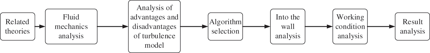
Figure 1: The research framework

2.2 Governing Equations of Fluid Mechanics

The heat dissipation phenomenon of a single transmission conductor under different wind speeds has been studied [15]. The theoretical method of fluid mechanics is mainly used since the research object involves wind and transmission single conductor. The air is considered to be a constant physical property, and the fluid is considered to be an unsteady Newtonian fluid. The two-dimensional method is adopted to simplify the problem to a certain extent. The thermal effect of viscous fluid is ignored here [16].

Eq. (1) presents the differential expression of mass conservation.

∂ρ∂t+∂(ρa)∂x+∂(ρb)∂y+∂(ρc)∂z=0 (1)

Eq. (1) expresses that the mass of the fluid flowing into and out of the area is the same at the same time. a, b and c are velocities, ρ is density, and t is time.

Eqs. (2)–(4) are expressions of the law of conservation of momentum.

∂(ρa)∂t+div(ρau)=∂p∂x+∂φxx∂x+∂φyx∂y+∂φzx∂z+ρfx (2)

∂(ρb)∂t+div(ρbu)=∂p∂y+∂φxy∂x+∂φyy∂y+∂τφzy∂z+ρfy (3)

∂(ρc)∂t+div(ρcu)=∂p∂z+∂φxz∂x+∂φyz∂y+∂φzz∂z+ρfz (4)

Eqs. (2)–(4) indicate that the increase of momentum of a certain volume of fluid at the same time is equal to the action of all environmental forces on it [17]. Where p is the pressure per unit volume of fluid, φxx, φxy, and φxz are the component of viscous stress in three directions [18], and f is the environmental force.

Eq. (5) is the expression of the energy conservation equation.

∂(ρT)∂t+div(ρuT)=div(kcpgradT)+VT (5)

Eq. (5) belongs to the first law of thermodynamics [19], which is applicable to all fluids where heat exchange may occur. Energy does not disappear, and it just shifts. The expression can be obtained by combining Eq. (5), that is, the change of fluid energy per unit volume is equal to the work done by the fluid in all aspects, where Cp is the specific heat capacity, T is the temperature, k is the heat transfer coefficient of fluid, and VT is the heat change of viscous fluid.

2.3 Implementation and Algorithm Selection of Turbulence Model

The choice of turbulence model plays an important role in the numerical simulation of flow [20]. The Reynolds number of single transmission conductors under common wind speed enters the subcritical region. Table 1 shows the relationship between Reynolds number and fluid flow state.

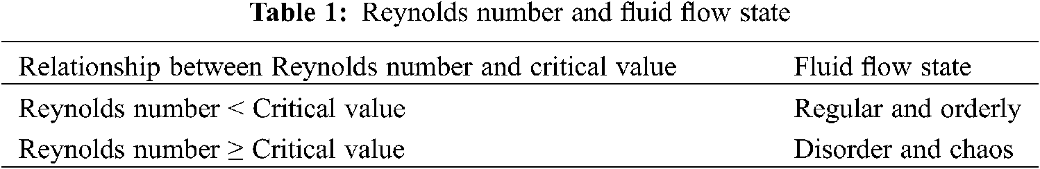
Table 1 suggests that the relationship between Reynolds number and critical value can indicate the flow state of the fluid. The fluid flow state studied is mainly turbulent flow, which is suitable for (Navier-Stokes equations) N-S equation and unsteady continuous equation. N-S is an equation of motion describing momentum conservation of viscous incompressible fluid. The equation of motion of viscous fluid was first proposed by Navier in 1827, which only considers the flow of incompressible fluid. Poisson put forward the equation of motion of compressible fluid in 1831. In 1845, Saint Venant and Stokes independently proposed the form of viscosity coefficient as a constant, which is called the N-S equation.

The numerical simulation of turbulent flow can be categorized into direct numerical simulation and indirect numerical simulation. The latter one is selected to solve the problem because of the large amount of calculation in the former one. It transforms the fluid in a turbulent state into a simpler model, and then carries out the calculation. It is divided into the large eddy simulation method and Reynolds average method. There are two kinds of models commonly used in turbulent flow: the Reynolds number stress model and the eddy viscosity model. The eddy viscosity model is adopted.

The eddy viscosity model includes zero-equation model, one-equation model and two-equation model.

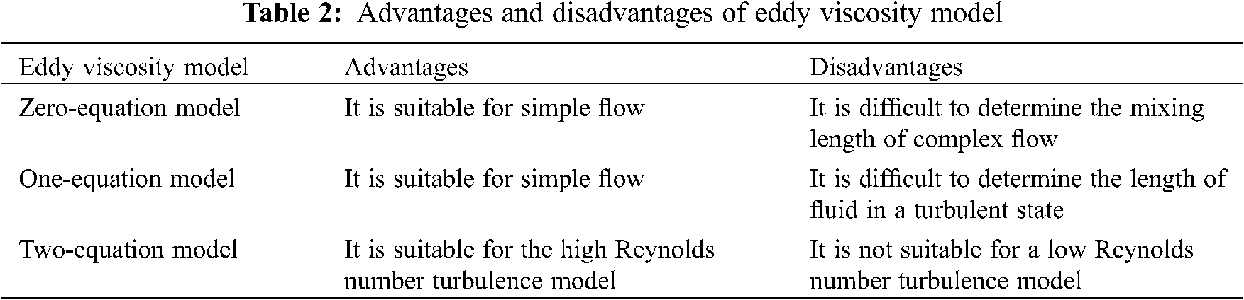
The two-equation model is selected according to the advantages and disadvantages of each model in Table 2. Near the wall, the k-ε model is used. The k-epsilon model is adopted for most fluid state regions. It is a kind of turbulence model theory, which is named the k-ε model in short. k-epsilon turbulence model is the most common turbulence model.

2.4 Near Wall Treatment

There are two kinds of flow states: eddy current and turbulent flow on the wall, so the solution on the wall exerts the greatest influence on the results. Near the wall, the fluctuation of horizontal velocity and vertical velocity decrease; in the region far away from the wall, the average velocity gradient increases and the turbulence increases. Fig. 2 presents the specific structure of the near-wall region.

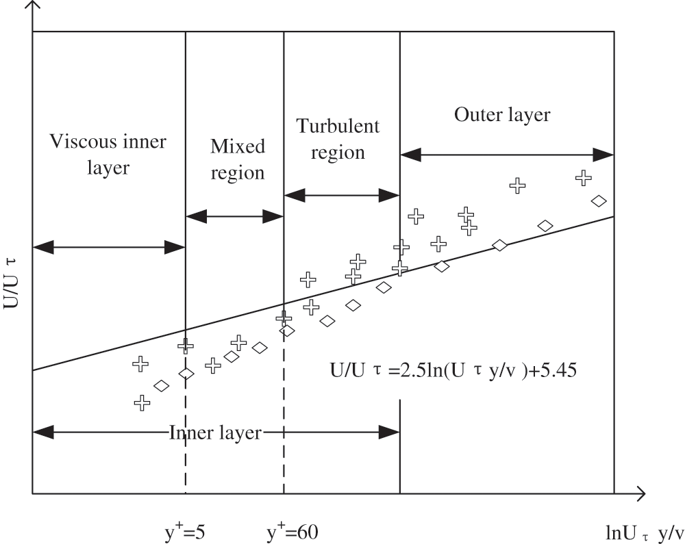
Figure 2: Structure of the near-wall region

Fig. 2 displays that the near-wall region is divided into the viscous layer, mixed region and turbulent region. Laminar flow is mainly distributed in the bottom region of the figure. Based on this, the viscosity of fluid molecules plays a crucial role in the momentum and heat of the fluid. Turbulent fluid is distributed in the outer layer of the figure, which plays the most crucial role in the whole turbulent flow state. The flow state of the fluid in the middle region of the figure is between turbulence and viscosity, and the effect of turbulent fluid in the middle region is the same as that of viscosity.

There are two ways to simulate the flow near the wall. One is wall function, and the other is refined net processing. The wall function is more accurate and convenient in solving the flow problem of fluid with a higher Reynolds number. However, the accuracy is higher by using the refined net processing for low Reynolds number fluid flow problems. The two methods are combined to solve the fluid flow near the wall.

In the near-wall area, the refined net method can achieve greater success in solving the accuracy. In order to better meet this requirement, two dimensionless parameters m+ and n+ are introduced to analyze the first layer of the grid structure. The equations are as follows:

m+=Utuτ=1kln(n+)+C (6)

In (6), m+ represents the velocity of the fluid in this state, and n+ represents the distance of the grid. Where, n+=ρΔnuτμ and uτ=(τwρ)1/2 . uτ represents the wall friction velocity, τw is the wall shear stress, and Δn is the wall distance. Here, n+ = 1 is used to represent the height of the first layer of the wall grid in the process of fluid flow.

SIMPLE algorithm (Semi-Implicit Method for Pressure Linked Equations) is a widely used numerical method for solving flow fields in CFD. It was proposed by Suhas V. Patankar and Brian Spalding in 1972. In the fluid flow state, the commonly used Fluent algorithms are Simple, Simplec, Coupled and so on. Because the Simplec algorithm is widely used and the coefficient of velocity correction equation is simple, the Simplec algorithm is used to analyze the fluid flow problem.

2.5 Discretization and Selection of Interpolation Methods

In Fluent software, the commonly used discrete methods are finite difference method, finite element method and finite volume method. The finite volume method has four following advantages. It has good conservation; more flexible assumptions can be set to overcome the shortcomings of Taylor expansion; it can solve complex engineering problems since it has good adaptability to the grid; it can perfectly integrate with the finite element method in the process of fluid structure coupling analysis. Based on the above four points, the finite volume method is applied to Fluent software to study and analyze the fluid. The algorithm of the finite volume method is expressed as follows. First, the corresponding computer domain is divided by the grid, and any control volume near the grid point must not be the same; then, each control volume is integrated under the control equation; finally, the corresponding fluid discrete equations are obtained.

The current interpolation methods include first-order upwind scheme, power-law scheme and second-order upwind scheme. The lower-order upwind schemes are generally stable and have fast convergence. Higher-order is more accurate than lower-order. Therefore, the method of combining low order and high order is adopted for calculation, which can not only meet the requirements of calculation accuracy, but also strengthen the convergence speed. When it is difficult to achieve a certain convergence speed by using high order interpolation algorithm, a low order scheme can be selected to calculate some parts, and then a high order scheme can be used to calculate.

3  Numerical Calculation of Flow Past Body and Heat Transfer around a Fixed Single Conductor

Here, first, the structure of transmission single conductor is introduced, as shown in Fig. 3.

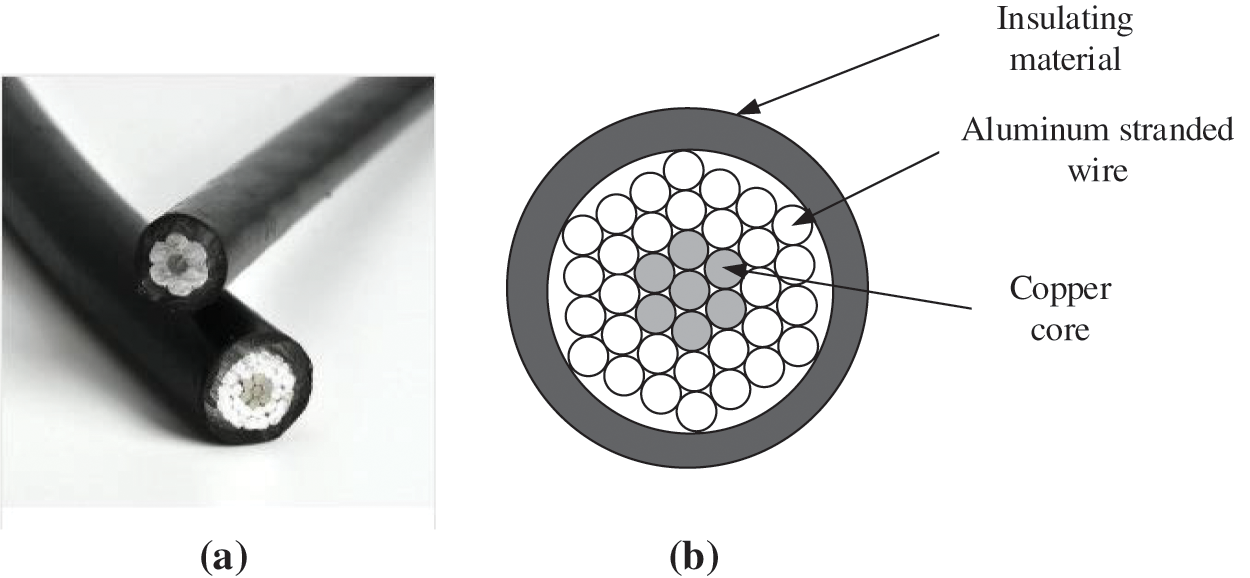
Figure 3: Structure diagram of transmission single conductor ((a) is the physical drawing of common transmission single conductor, and (b) is the specific composition of transmission single conductor)

Fig. 3a is a physical drawing of a common transmission single conductor. Fig. 3b shows that the transmission single conductor consists of three parts: the outermost insulating material, the aluminum stranded wire in the middle layer and the innermost copper core. Aluminum stranded wire mainly plays the role of transmitting electric energy. It is wound around the copper core in the form of stranding, and the innermost copper core plays the role of increasing strength.

Algorithm simulation is conducted for the flow past body and heat transfer characteristics of the single transmission conductor. The wind speed range 1~7 m/s is selected, and the Fluent software is adopted to simulate the steady-state; second, the steady-state simulation results are compared with the literature results, and the results show that the CFD numerical method has a certain accuracy; finally, two different boundary conditions are used to make the constant heat flow state and the constant wall temperature state respectively. The Nusselt number under these two conditions is compared and analyzed, and the difference is mainly studied. The laminar flow model and SST model are adopted for related numerical simulation of the low Reynolds number model and the corresponding Reynolds number of subcritical region.

3.1 Computation Model

The CFD model needs a large computational area to represent the real fluid flow state. In the numerical simulation, it is essential to choose the correct calculation domain, so that the accuracy and efficiency can be satisfied.

The following numerical calculation domain is selected based on the related literature. The calculation domain of the rectangular flow field of the two-dimensional model is 40R × 25R. The distance between the central entrance of the cylinder as a single conductor is 30R, and the distance between the upper and lower boundaries of the whole region is 25R. The circular region 4R represents the grid region, and its density is increased. Here, setting a certain range of dense areas is to achieve higher accuracy; moreover, it is more convenient for different grids to use different divisions.

The fluid velocity selected is uniform turbulent fluid, and the boundary condition at the grid entrance meets the requirement of fluid velocity. The flow velocity of inlet fluid is controlled by the computer program to better meet the requirements of calculation accuracy. The selection of wind speed is the same as the previous part. Uniform wind speed is selected to simplify the problem. The intensity of the fluid turbulence state should be calculated by 1%. The fluid is free at the exit boundary of the grid and is not constrained. The research state is ideal, and the cylinder surface exerts little influence on the research results. Hence, the upper and lower walls of fluid flow are regarded as free sliding walls, and the single conductor cylinder wall is regarded as non-sliding walls.

3.2 Meshing

At present, there are mainly triangular grids and rectangular grids. The former has lower accuracy and convergence than the latter. However, the former is more convenient than the latter. The rectangular grid is chosen to calculate for the sake of accuracy and convergence. ICEM software is adopted to divide the rectangular grid. Because of the medium and fast characteristics of the software, the circular subdivision method is employed to divide the rectangular calculation area. The growth rate of the 3R circular dense region around the single conductor is slow, and the growth rate of the rectangular grid in the second half of fluid flow should be widened.

The density of the rectangular grid is increased as follows. To achieve a certain accuracy, the SST model is adopted when the Reynolds number increases to the subcritical range. The rectangular grid near the wall is adjusted to the densified state.

The control of the first layer edge network in the 3D circular area is n+ = 1, and the length from the first layer of rectangular grid to the wall of the single conductor cylinder is n. Eq. (7) presents the calculation equation.

Re=vra,n+=0.172nLRe0.9 (7)

In (7), Re is the Reynolds number, v is the velocity of fluid inflow, r is the diameter of the single conductor wire, and a is the viscosity of fluid flow state.

The grid encryption principle selected is the double principle, and the number of grids after encryption is twice that before encryption. The “scale factor” function in CFD software is used for grid encryption, and the actual network parameters are obtained by multiplying it by the set parameters. In order to achieve this goal, it is only necessary to change the encrypted side length to the original (1/2)1/3, which is about 0.7937. The second encryption changes the scale factor to 0.79372. The value of scale factor is 0.7937n. Based on Grid 1 and according to the above principles, Grid 2 and Grid 3 are generated until Grid 5. Each drawn grid is smoothed to ensure grid quality. Calculate each grid with fluent and observe the relative static pressure at the outlet. The wind velocity is selected between 1.0 and 7.0 m/s, so the inlet velocity is first taken as 1.0 m/s. For subsonic flow, the velocity inlet boundary condition directly ignores the pressure. Therefore, there is no pressure condition in the simulation. The characteristic velocities are 1, 2, 3, 4, and 5 m/s, respectively, and the temperature is monitored at the outlet of the model. Grid sensitivity analysis is shown in Table 2. The results in Table 2 lay the foundation for the later results.

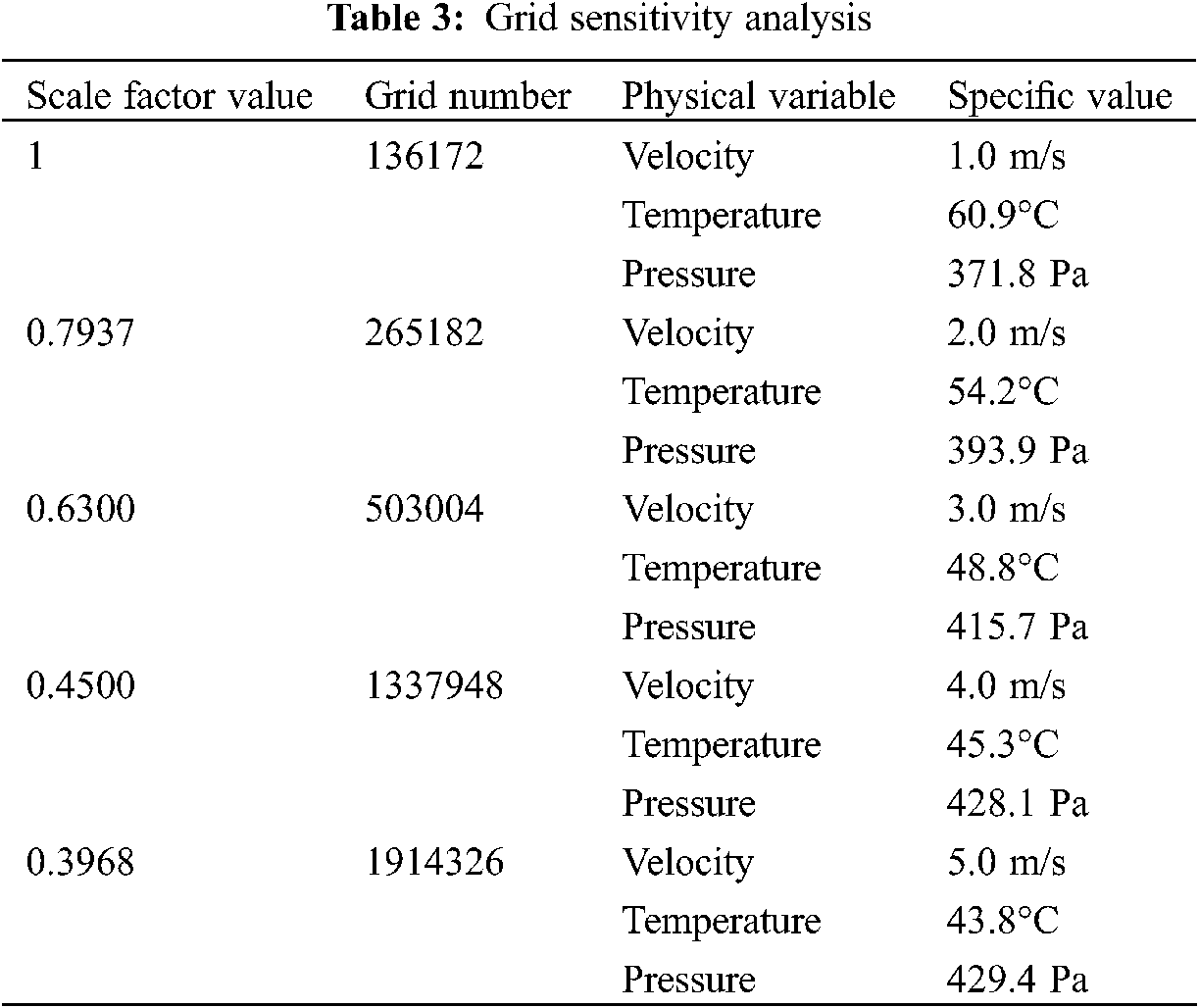
Table 3 suggests that, when the number of grids reaches 1337048, the outlet pressure gradually tends to be stable. From Grid 4 to Grid 5, the change of outlet pressure is very small, and the change of outlet temperature is consistent with the outlet pressure, indicating that when the number of grids reaches 1337948, increasing the number of grids will not significantly improve the calculation accuracy. Therefore, it can be judged that grid 4 has met the calculation requirements to a certain extent.

3.3 Working Condition Selection

The selected wind speed range is 1~7 m/s and the Reynolds number range is 467~10064. The laminar flow model is applied when the fluid is in the low Reynolds number range, and the SST turbulence model is applied when the fluid is in the high Reynolds number range. Second-order is adopted to adjust different pressures. LGJ210/20 wire is used for the single conductor.

The outer diameter of the conductor is 21.6 mm, Ie/A is 450, and the DC resistance of the conductor Ω is 0.1181 km. The state of the fluid is air, the regional temperature of the fluid is 21°C, and the air density is ρ = 1.205 kg/m3. The kinematic viscosity coefficient is v = 1.506 × 10−5 m2/s, the dynamic viscosity is μ = 1.81 × 10−5 kg/ms, Cp = 1.005 KJ/(KgK), λ = 0.0259 W/(mK), and Prandtl coefficient is Pr = 0.728.

The boundary condition of the transmission line belongs to the constant heat flow boundary condition. First, the fluid flow characteristics under the condition of constant wall temperature are calculated, and the calculation results are compared with the research equations in the literature; then, the constant heat flow boundary is studied and calculated under the same conditions as constant wall temperature; finally, the calculation results of the former and the latter are plotted and analyzed. The boundary temperature at constant wall temperature is set at 349.15 K, and the fluid at constant heat flow is calculated by density. Eq. (8) is the density calculation method of a single conductor fluid under constant heat flow.

q=S2Rπr (8)

In Eq. (8), S is the current carrying capacity of a single transmission conductor, R is the resistivity of single transmission conductor, and R is the diameter of a single transmission conductor.

Eq. (9) is the definition of the local Nusselt number of the cylindrical surface.

Nuθ(θ,t)=−rTw−T∞∂T∂r=−∂T¯∂r|R=0.5,Nuθ(θ)¯=1hp∫0hp⁡Nuθdt (9)

Eq. (9) is adopted to evaluate the heat transfer condition of the conductor under the same working condition. hp is the oscillation period of the conductor.

4  Analysis on Research Results of the Flow Past Body and Heat Transfer Characteristics of the Fixed Single Transmission Conductor

4.1 Flow Past Body Characteristics under Different Wind Speeds

The flow past body characteristics of a fixed single cylinder are closely related to the variation of Reynolds number. The time history curve of lift and resistance coefficients is obtained by simulating the wind speed range of 1~7 m/s and the Reynolds number range of 467~10064. Due to the limited space, the lift coefficient diagram and resistance coefficient diagram under 1.0 m/s wind speed and 5.0 m/s wind speed are drawn here, as shown in Fig. 4.

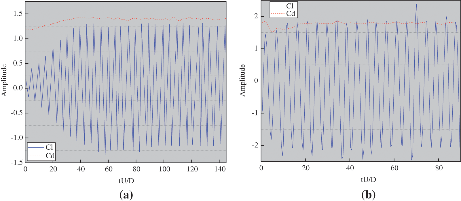
Figure 4: Curves of lift and resistance coefficients of fluid at 1.0 m/s (a) and 5.0 m/s (b)

Figs. 4a and 4b are the curves of the lift and resistance coefficients of the fluid under the wind speed of 1.0 and 5.0 m/s, respectively. The two figures reveal that the lift coefficient tends to be stable after reaching 40.

Figs. 5 and 6 are the average temperature change and temperature cloud chart of the conductor.

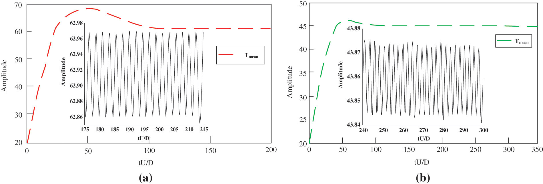
Figure 5: Average temperature change of fluid conductor under wind speed of 1.0 m/s (a) and 5.0 m/s (b)

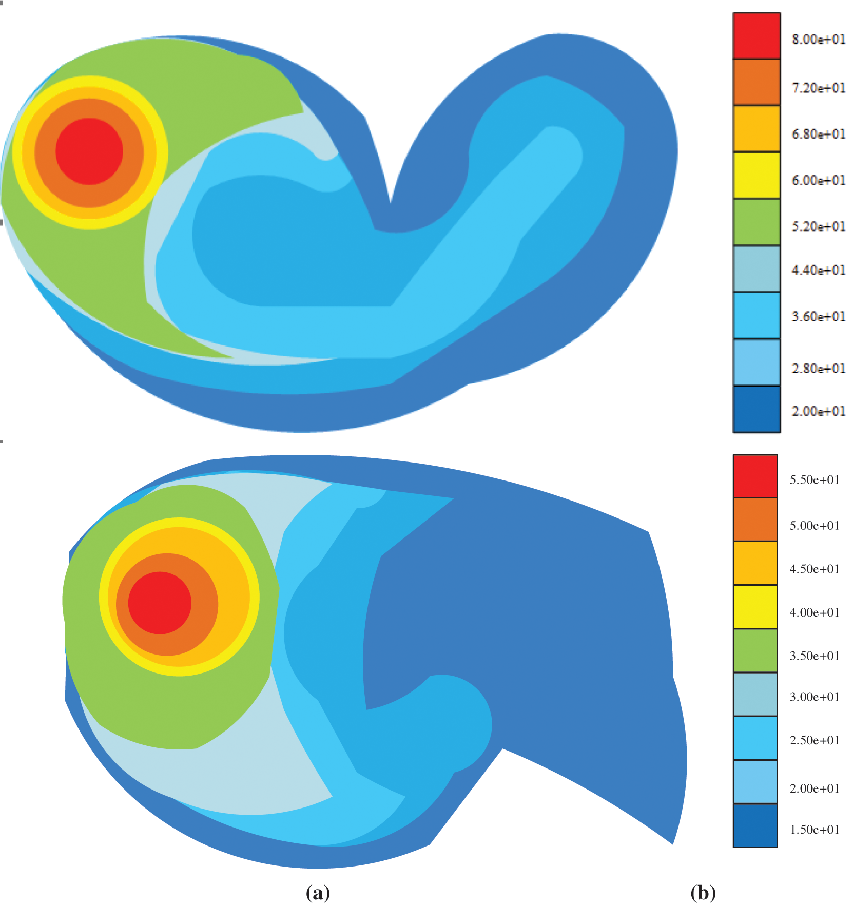
Figure 6: Conductor temperature cloud chart of fluid under wind speed of 1.0 m/s (a) and 5.0 m/s (b)

Figs. 5 and 6 show that the average temperature of the conductor is about 60.92°C when the wind speed is 1.0 m/s, and that is about 43.86°C when the wind speed is 5.0 m/s. The average temperature of the conductor decreases with the increase of wind speed. In this experiment, the conductor temperature under the wind speed of 1~7 m/s is measured, and only the conductor temperature under the wind speed of 1.0 m/s and 5.0 m/s is given here. The results show that the conductor temperature decreases gradually under the wind speed of 1~5 m/s, but the conductor temperature does not decrease significantly under the wind speed of 5~7 m/s, indicating that the wind speed has limitations on the reduction effect of conductor temperature; the heat generated by the resistance of the conductor itself has been fully diffused with the increase of wind speed.

FFT technology is employed to operate the lift coefficients in Figs. 7a and 7b to obtain the spectrum of the two wind speeds. Fig. 7 displays the result.

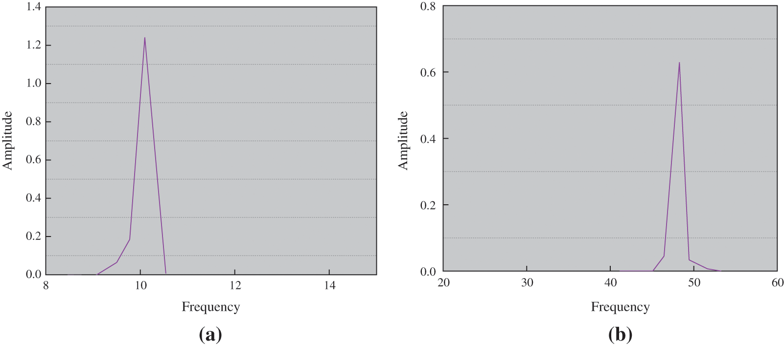
Figure 7: Frequency spectrum of lift coefficient at 1.0 m/s (a) and 5.0 m/s (b)

Figs. 7a and 7b suggest that the vortex shedding frequency changes with the change of Reynolds number. Previous studies have shown that the stress and heat transfer characteristics of transmission single conductors are affected by vortex shedding frequency.

Figs. 8 and 9 show the lift coefficient and resistance coefficient under different wind speeds. The lift coefficient of the fluid in the figure is calculated by the amplitude, the resistance coefficient is calculated by the mean value, and the results are compared with those in the literature.

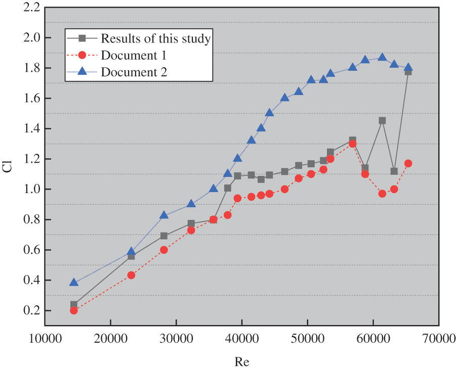
Figure 8: A curve of the lift coefficient changing with reynolds number

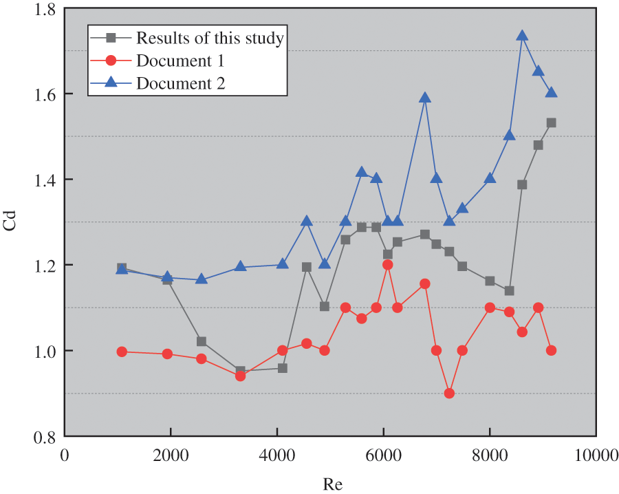
Figure 9: A curve of the resistance coefficient changing with reynolds number

Fig. 8 shows that the lift coefficient increases with the increase of Reynolds number in the simulation range. Finally, it tends to be stable in the Reynolds number range of about 4000. The lift coefficient fluctuates around 1.6. By comparing the data in the literature, it can be concluded that the calculated results are close to those in literature 1 when the Reynolds number is less than 2000. With the increase of Reynolds number, the simulation results are between Literature 1 and Literature 2.

In Fig. 9, unlike the lift coefficient, it has been found that the resistance coefficient is not affected by the Reynolds number. The simulation results are between Literature 1 and Literature 2.

4.2 Results of Nusselt Number for Different Wind Speeds

Two-dimensional models are selected. In the wind speed range of 1~7 m/s, the increase or decrease of the Nusselt number is calculated, and the time history of the Nusselt number at different Reynolds numbers is obtained. Fig. 10 is the time history curve of constant wall temperature under two kinds of wind speed.

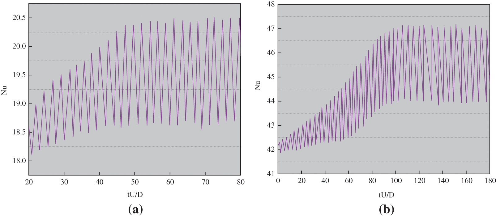
Figure 10: Time history curve of wall heat transfer at 1.0 m/s (a) and 5.0 m/s (b)

Fig. 10 presents the relationship between the circular cylinder as well as vortex shedding and heat transfer characteristics of a single conductor. After Figs. 10a and 10b are compared, it is obvious that the increase of wind speed increases the amplitude of the Nusselt number. After the wind speeds of 1.0 and 5.0 m/s are compared, it can be seen that the amplitude of the Nusselt number corresponding to 1.0 m/s is 20, and the amplitude of the Nusselt number corresponding to 5.0 m/s is 45. When the Nusselt number curve tends to be stable, the average Nusselt number of one cycle is adopted to show the heat transfer at the corresponding Reynolds number. The results are summarized in Fig. 11. The empirical equations for comparison in Fig. 11 are shown in Eqs. (10)–(12).

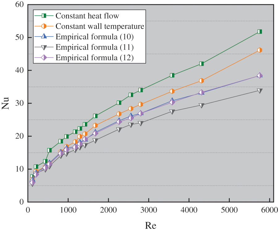
Figure 11: Nusselt number results of circular cylinder

Nu=0.51Re0.5 (10)

Nu=0.683Re0.466Pr1/3 (11)

Nu=0.3+0.62Re1/2Pr1/3[1+(0.4/Pr)2/3]1/4[1+(Re28200)5/8]4/5 (12)

Eqs. (10)–(12) are three different boundary simulation equations for constant heat flux and constant temperature wall of a fixed single cylinder. Re is Reynolds number, Nu is Nusselt Number, and Pr is Prandtl constant. Fig. 11 suggests that the Nusselt number at constant wall temperature is smaller than that at constant heat flow. When the Reynolds number is small, the difference of Nusselt number between constant wall temperature and constant heat flow is small. When the Reynolds number is less than 1500, the calculated results of the three references are almost the same. The calculated results are close to the literature equation at constant wall temperature. With the increase of Reynolds number, there is a certain deviation in the calculation results of the three empirical equations.

It has been found that the laminar flow of a single conductor at a certain temperature is close to the results of the literature equation, and the calculation results in the turbulent state are higher than those in the literature. It is preliminarily speculated that the influence of turbulence degree is the main reason.

The Nusselt number and Reynolds number are compared under constant heat flow. Fig. 12 displays the fitting results.

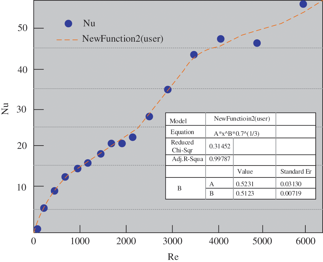
Figure 12: Fitting results of constant heat flow Nu with Reynolds number

Fig. 12 suggests that the fitting results are: Nu=CRenPr1/3 , C = 0.5331, and n = 0.5123. The analysis shows that the range of the Reynolds number is 500~6000.

To sum up, the flow past body and heat transfer characteristics of the fixed single conductor are summarized as follows. Under different wind speeds, the average Nusselt coefficient will gradually increase with the increase of wind speed, and the increase is more obvious when Re ≤ 2000. The lift coefficient tends to be stable after reaching 40 at 1.0 and 5.0 m/s. The Nusselt number at constant wall temperature is smaller than that at constant heat flux. The difference of Nusselt number between constant wall temperature and constant heat flux is small when the Reynolds number is small.

5  Conclusion

Based on the principle of fluid mechanics, two kinds of characteristics of the single transmission conductor are studied and analyzed by using relevant computer software. The flow past body and heat transfer characteristics of the single transmission conductor are mainly studied and analyzed. The main research results are as follows:

(1)  The flow past body characteristics of the fixed single conductor at a wind speed of 1~7 m/s are studied. The results are compared with the existing research results to verify the accuracy of the numerical simulation. The flow past body characteristics depend on the Reynolds number. In the simulation range, the lift coefficient increases with the increase of Reynolds number, and reaches a stable value of 1.6 when Reynolds number is about 4000. The drag coefficient fluctuates little with the Reynolds number.

(2)  The heat transfer characteristics of the single transmission conductor under 1~7 m/s wind speed are studied. The results show that the Nusselt number is affected by the Reynolds number, and the whole process is nonlinear. The Nusselt number increases slowly when the Reynolds number is more than 3000. The Nusselt number at constant wall temperature is smaller than that at constant heat flow. When the Reynolds number is small, the difference of Nusselt number between constant wall temperature and constant heat flow is small.

(3)  The two-dimensional model is used, while the influence under the three-dimensional situation is ignored, so there may be some errors. In future research, it is essential to combine the three-dimensional model for specific analysis to meet the actual situation.

Due to the limitations of research conditions and funding, turbulence intensity is considered as a lower value in the simulation study. However, in the actual situation, the different geomorphic environments will exert different degrees of impact on turbulence, so it is essential to consider the impact of turbulence on VIV and heat transfer characteristics in combination with different geomorphic characteristics. Besides, only the influence of wind speed is considered, and the influence of external factors such as light on heat transfer of unidirectional conductors is not considered, which is the research limitation. More influencing factors will be considered and more comprehensive research will be conducted in future research.

Funding Statement: The authors received no specific funding for this study.

Conflicts of Interest: The authors declare that they have no conflicts of interest to report regarding the present study.

This work is licensed under a Creative Commons Attribution 4.0 International License, which permits unrestricted use, distribution, and reproduction in any medium, provided the original work is properly cited.