Fluid Dynamics & Materials Processing

DOI: 10.32604/fdmp.2022.017508

ARTICLE

Numerical Investigation on the Aerodynamic Noise Generated by a Simplified Double-Strip Pantograph

Jiawei Shi1, Shuai Ge1 and Xiaozhen Sheng2,*

1State Key Laboratory of Traction Power, Southwest Jiaotong University, Chengdu, 610031, China
2School of Urban Railway Transportation, Shanghai University of Engineering Science, Shanghai, 201620, China
*Corresponding Author: Xiaozhen Sheng. Email: shengxiaozhen@hotmail.com
Received: 15 May 2021; Accepted: 08 September 2021

1  Introduction

With the continuous increase in train operation speed, train noise pollution becomes more and more serious. The noise radiated by high-speed trains seriously affects the life of residents along the line. It is urgent to take effective measures to reduce the noise levels of high-speed trains. The high-speed train noise mainly includes wheel/rail rolling noise and aerodynamic noise. It is generally believed that the aerodynamic noise increases with the speed faster than the wheel/rail rolling noise. According to the test results in Europe, when the speed exceeds 300 km/h, the aerodynamic noise will exceed the wheel/rail noise and occupy a dominant position [1,2]. As a prominent part on the roof of the high-speed train, the pantograph is directly impacted by high speed air flow, with high noise intensity, which is the local strongest noise source of a high-speed train [3]. Besides, as the pantograph is located on the train roof, the aerodynamic noise of the pantograph will be more prominent for the lines with sound barriers [1]. Therefore, the problem of pantograph aerodynamic noise has attracted the attention of many scholars and engineers.

There are two main methods for pantograph aerodynamic noise research, experiment and numerical simulation. In terms of experimental research, Noger et al. [4] tested the aerodynamic noise of TGV train pantograph system in low-noise wind tunnel and found that the vertical plane at the rear of the pantograph cavity is the main noise source, and the presence of pantograph will increase the amplitude of broadband noise. Different from the general cavity flow, there is no cavity resonance in the pantograph cavity. Lauterbach et al. [5] conducted aerodynamic noise test for a 1:25 ICE train scale model in wind tunnel, and found that all single frequency sound in noise arise from the top area of the pantograph. Lölgen et al. tested the aerodynamic noise of two different types of pantograph, DSA350SEK and ASP in the wind tunnel. He found that the single frequency sound in the noise spectrum is related to the vortex shedding of the cylindrical components of the pantograph and determined the source of the peak values by Strouhal criterion [6]. Brick et al. [7] tested the aerodynamic noise of pantograph installed in the concave cavity under the state of raised and folded. The results show that the noise of the raised pantograph is 8 dB higher than the folded one. Lee et al. [8] investigated the wake and aerodynamic forces of a double-arm, a single-arm and a periscope-arm pantograph with a rectangular panhead and an optimized panhead through wind tunnel test. Chen et al. [9] investigated the influence of pantograph shroud on the aerodynamic noise of pantograph through wind tunnel test. The results show that the shroud has little effect on the overall sound pressure level when the pantograph is raised, while it has a good noise reduction effect when the pantograph is folded.

Although the aerodynamic noise results of pantograph under real conditions can be obtained by experimental research, the cost of experimental research is high and the flow field information can be obtained is limited. With the rapid development of computing technology, computational fluid dynamics (CFD) technology is gradually applied to the prediction of aerodynamic noise. More comprehensive flow field information can be obtained through numerical simulation, which can help people understand the mechanism of aerodynamic noise more deeply. In the aspect of numerical simulation, Yu et al. [10] applied the non-linear acoustic solver (NLAS) combined with FW-H equation to analyze the aerodynamic noise characteristics of a simplified DSA-350 pantograph and the noise reduction effects of four different designs of pantograph fairing. They found that the aerodynamic drag of pantograph area would be increased by all four schemes, and only the scheme using side sound insulation panels could reduce the noise of pantograph. Ikeda et al. [11] used CFD method and described the shape of panhead section with B-spline curve, to optimize the panhead section shape combined with optimization algorithm. The new panhead shape has better aeroacoustic and aerodynamic performance. Meskine et al. [12] calculated the aerodynamic noise of a full-scale four car high-speed train model by using lattice Boltzmann method based software PowerFLOW. The results show that for the measuring point 7.5 m away from the track, the pantograph is the main aerodynamic noise source in the frequency range of 200∼400 Hz and above 800 Hz. Zhang et al. [13,14] analyzed the aerodynamic noise characteristics of a DSA-380 pantograph through numerical simulation and they further studied the influence of cross wind on aerodynamic noise of pantograph. Tan et al. [15] analyzed the spatiotemporal evolution of vortex structures in the unsteady flow field of the CX-PG pantograph through numerical simulation, and studied the relationship between the vortex structures and the aeroacoustic performance of the pantograph components. Noh simulated the flow field and aerodynamic noise of a real-scaled CX-PG pantograph and analyzed the generation mechanism of its aerodynamic noise by using PowerFLOW software [16]. Kim et al. [17,18] investigated the influence of pantograph cavity on the flow field and aerodynamic noise of pantograph area by numerical simulation. Li et al. [19] studied the effect of the strip spacing on the aerodynamic noise characteristics of the pantograph by numerical simulation, an important conclusion is that the single-strip pantograph has better aerodynamic and aeroacoustic performance than double-strip pantograph.

The purpose of this paper is to analyze the relationship between the vortex structures in the pantograph area and the pressure fluctuation(dipole source) on the surface of the pantograph to explore the generation mechanism of pantograph aerodynamic noise and master the far-field aerodynamic noise characteristics of the pantograph, including the spatial distribution characteristics of the far-field noise, the noise contribution of each component, the spectrum characteristics and the inflow velocity dependent regularity. Therefore, a simplified double-strip pantograph is taken as the research object. The unsteady flow field around the pantograph is simulated by LES model, and the far-field aerodynamic noise is calculated by FW-H equation. The arrangement of the paper is as follows. In Section 2, LES model, FW-H acoustic analogy equation and its integral solution are introduced. In Section 3, the geometry model, mesh scheme and solution setup are introduced. In Section 4, the fluctuating pressure (dipole source) on the pantograph surface and the unsteady vortex structures in the pantograph flow field are analyzed, and the relationship between them is discussed. In Section 5, the far-field aerodynamic noise characteristics of pantograph are studied. Finally, Section 6 summarizes the whole paper and gives the main conclusions.

2  Mathematical-Physical Model

As the large eddy simulation (LES) model has a strong ability to capture vortices, it is first used to calculate the flow field around the pantograph to obtain accurate sound source data. Then the FW-H equation is used to calculate the far-field aerodynamic noise of the pantograph.

2.1 LES Model

Large eddy simulation is a kind of spatial averaging of turbulent fluctuations. Its basic idea is to separate the large-scale vortices and small-scale vortices through filtering function, the large scale vortices are solved directly, while small scale vortices are solved by modeling. The governing equations employed for LES are filtered Navier-Stokes equations, which are as follows:

∂ρ∂t+∂(ρu~j)∂t=0 (1)

∂(ρu~i)∂t+∂(ρu~iu~j)∂t=−∂p~∂xi+∂σij∂xj+∂τ~ij∂xj (2)

where the overline represents the average value of the physical quantities in the spatial domain, ρ is the fluid density, t is time, u is the fluid velocity, p is the pressure, σij is the viscous stress tensor, and τ~ij is the sub-grid stress tensor. To realize large eddy simulation, it is necessary to construct a sub-grid stress model. In this paper, The Smagorinsky-Lilly sub-grid stress model is used, which is in the form of:

τ~ij=13τ~kkδij−2μtS~ij (3)

where μt is the sub-grid viscosity coefficient and S~ij is the strain rate tensor, δij is Kronecker tensor, and the viscosity coefficient of sub-grid turbulence can be expressed as:

μt=ρLs|S~| (4)

and

Ls=min(κd,CsV1/3) (5)

where Ls is the mixed length of the grid, κ is the von Karman constant, d is the nearest distance from the grid to the wall, Cs is the Samagorinsky constant, and V is the volume of the computational element.

2.2 FW-H Equation

In 1969, Fwowcs Williams and Hawkings extended Lighthill and Curle’s results to consider the influence of the moving solid boundary by introducing generalized functions, and obtained a more general result-FW-H equation, as shown in Eq. (6) [20]:

1c02∂2∂t2[p′H(f)]−∇2[p′H(f)]=∂∂t[ρ0vn|∇f|δ(f)]−∂∂xi[pijn^j|∇f|δ(f)]+∂2∂xi∂xj[TijH(f)] (6)

where c0 is the sound speed, p′ is the sound pressure, x is the component of the Cartesian coordinate, f = 0 is the equation of the sound source surface. H(∙) is Heaviside function, ρ0 is the density of the fluid at the undisturbed area, ∇ is Nabla operator, vn is the normal velocity component of the sound source surface, Tij is the Lighthill stress tensor.

If the right hand of Eq. (6) is regarded as the source term, Eq. (6) is a typical wave equation. The three terms at the right hand of the equation represent monopole source term, dipole source term and quadrupole source term respectively. In this paper, the quadrupole source term is ignored, because in the low Mach number flow, compared with the other two source terms, the contribution of quadrupole is negligible, which has been verified in the aerodynamic noise prediction of landing gear, high-speed train bogie and other low Mach number flow conditions [17,21–23]. Besides, the pantograph is in the static state in the numerical simulation, the monopole source is also 0. In this case, the far-field noise of pantograph only includes the contribution of dipole source term. Solving FW-H equation by using Green’s function in free space, the time domain integral solution of FW-H equation is obtained as follows:

p′=14π∫f=0(Lij⋅⁡njr^ic0r+Lijnjr^ir2)τ=τedS (7)

with

Lij=(p−p0)δij−σij (8)

where r is the distance from a point on the surface of the sound source to the receiving point, and the subscript τ = τe indicates that the relevant variables are evaluated at restarted time τe, and τe = r/c0, nj is the unit outward normal vector of a point on the sound source surface, and r^i is the unit vector from the source point to the receiving point. p0 is the pressure of the fluid in the undisturbed area. It should be noted that the influence of air flow on sound propagation is not considered when Eq. (7) is used to calculate the far-field aerodynamic noise of pantograph.

3  Simulation Model

3.1 Geometry Model

A simplified full scale double-strip pantograph model is used as the research object, and its geometry model is shown in Fig. 1. Compared with the complex pantograph model, the simplified model with the main structural features can reduce the number of grids and help to obtain high quality grids, which can reflect the flow field characteristics of the pantograph area and at the same time improve the computational efficiency.

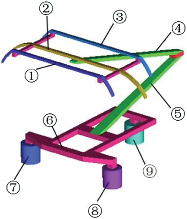
Figure 1: Geometry model ①-strip1; ②-balance arm; ③-strip2; ④-upper arm; ⑤-lower arm; ⑥-base frame; ⑦-insulator1; ⑧-insulator2; ⑨-insulator3

3.2 Mesh Scheme

A rectangular computational domain in Fig. 2 is used to simulate the external flow field of the pantograph. The distance from the bottom center of the pantograph to the inlet of computational domain is 9 m, to domain outlet is 25 m and to domain top and side are 7.5 m. The distance between the pantograph and the outlet of the computational domain is more than 10 times length of the pantograph, which ensures that the influence of the wake of the pantograph on the outlet boundary can be ignored. The distance from the pantograph to the two sides and the top of the computational domain is close to five times of the height and width of the pantograph respectively, which ensures that the blocking ratio of the numerical wind tunnel is around 1%. The maximum mesh size of pantograph surface is set as 5 mm, and 17 layers of fine prism layer mesh with initial height of 0.01 mm and growth rate of 1.2 are drawn on the surface of pantograph. Two blocks are set up to refine the mesh. Three sets of mesh are divided by modifying the mesh size of the encryption domain, which are named coarse, medium and fine mesh. When the mesh size in the first block around the pantograph is 20 mm, 10 mm and 5 mm, respectively, the corresponding grid numbers of three sets of mesh are approximately 8 million, 17 million and 32 million. Fig. 3 shows the computational mesh and encryption blocks (yellow dotted line).

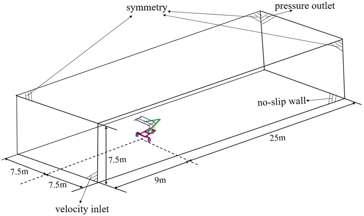
Figure 2: Computational domain

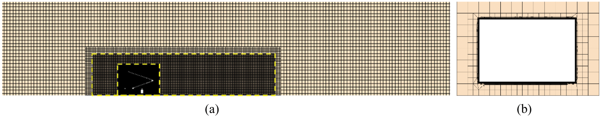
Figure 3: Computational mesh. (a) Mesh distribution of middle section (b) Prism layers of strip

3.3 Solution Setup

The maximum inflow velocity is 400 km/h and the corresponding Mach number is 0.327. There are two main reasons for still considering air as incompressible gas in this paper. One is that Mach number is still close to 0.3, and the compressibility of gas is not strong; the other is that it is difficult to accept the computing resources and time cost required for using the compressible model, and the incompressible gas model has better convergence and calculation efficiency. The inlet of the computational domain is set as velocity inlet boundary and flow velocity is input, the outlet of the computational domain is set as pressure outlet boundary, the static pressure is 0, the two sides and the top of the computational domain are set as symmetrical boundary condition, the bottom of the computational domain and the pantograph surface are set as the static wall with no slip.

The steady flow field computation combined the Realizable k − ε turbulence model and non-balance wall treatment method [24]. The pressure velocity coupling used the Semi-Implicit Method for Pressure Linked Equations (SIMPLE) algorithm. The continuity equation is discretized using the standard scheme. The momentum equation, turbulence kinetic energy equation, and turbulence dissipation rate equation are discretized using the second-order upwind scheme. The transient flow field computation used the LES model. The temporal difference equation used a second-order implicit scheme. The pressure-velocity coupling used the Pressure-Implicit with Splitting of Operators (PISO) algorithm. The continuity equation is discretized using the PRESTO! scheme. The momentum equation is discretized by using bounded central differencing scheme.

The convergent steady-state results provide initial field for transient simulation. The time step of transient calculation is 10−4 s, according to Nyquist theorem, the corresponding maximum analysis frequency being 5000 Hz. Each time step has 20 iterations to ensure convergence. During the transient calculation, the first 1500 time steps ensure flow field achieve statistical stability, and the next 2500 time steps record the fluctuating pressure data on the pantograph surface as the calculation input of far-field noise.

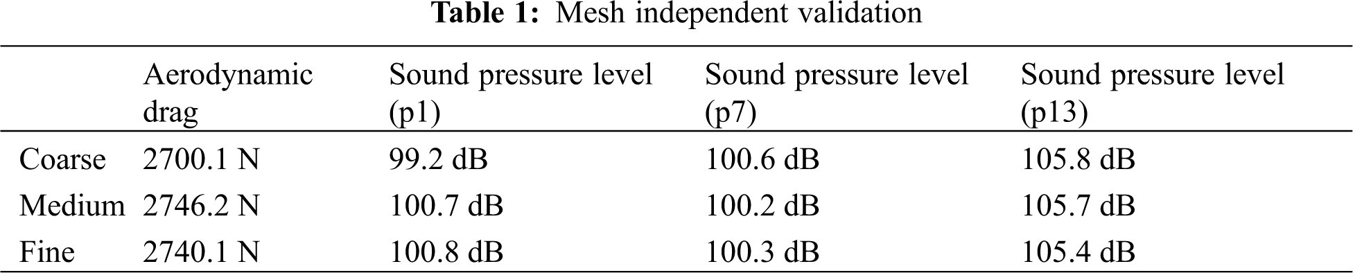
3.4 Mesh-Independent Validation

Table 1 shows the aerodynamic drag of the pantograph and the sound pressure level results of three far-field measuring points (see Fig. 10 for the location of measuring points) by using three sets of mesh based on the calculation process above. It can be seen from the results that the relative difference of aerodynamic drag between medium grid and fine grid is less than 2%, and the difference of sound pressure level is less than 0.5 dB, which indicates that when the mesh reaches the medium mesh scale, the computation results are independent of the grid distribution. Therefore, the medium mesh is used in this paper.

3.5 Verification of Calculation Methods

According to the solution setup mentioned above, the aerodynamic noise generated by a cylinder with a diameter of 10 mm at inflow velocity of 72 m/s is simulated. This case is also used to verify the calculation method in other literatures on pantograph aerodynamic noise research [10,19,25]. Fig. 4 shows the calculation conditions and the computational mesh. The simulation results are compared with the experimental results in the literatures [26,27]. Fig. 5a shows the time-averaged pressure coefficients on the cylinder surface. Fig. 5b shows the spectrum of sound pressure level at the measuring point 1.85 m away from the center of the cylinder in the vertical direction. In the numerical simulation, the time step is set as 5 × 10−5 s, and the sampling time is 0.25 s, corresponding to the frequency resolution of 4 Hz, which is the same as that of the experiment. It can be seen that the time-averaged pressure coefficient obtained by numerical simulation and the experimental results agree well, and the numerical simulation could capture the peak value caused by periodic vortex shedding. In general, the simulation results are in good agreement with the experimental results, which verifies the reliability of the calculation methods in this paper.

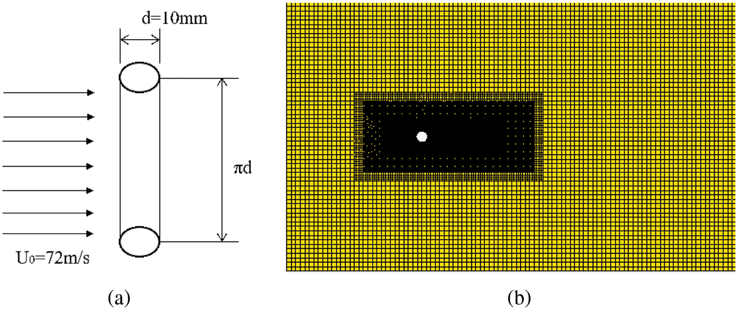
Figure 4: Aerodynamic noise model of a cylinder (a) calculation conditions (b) computational mesh

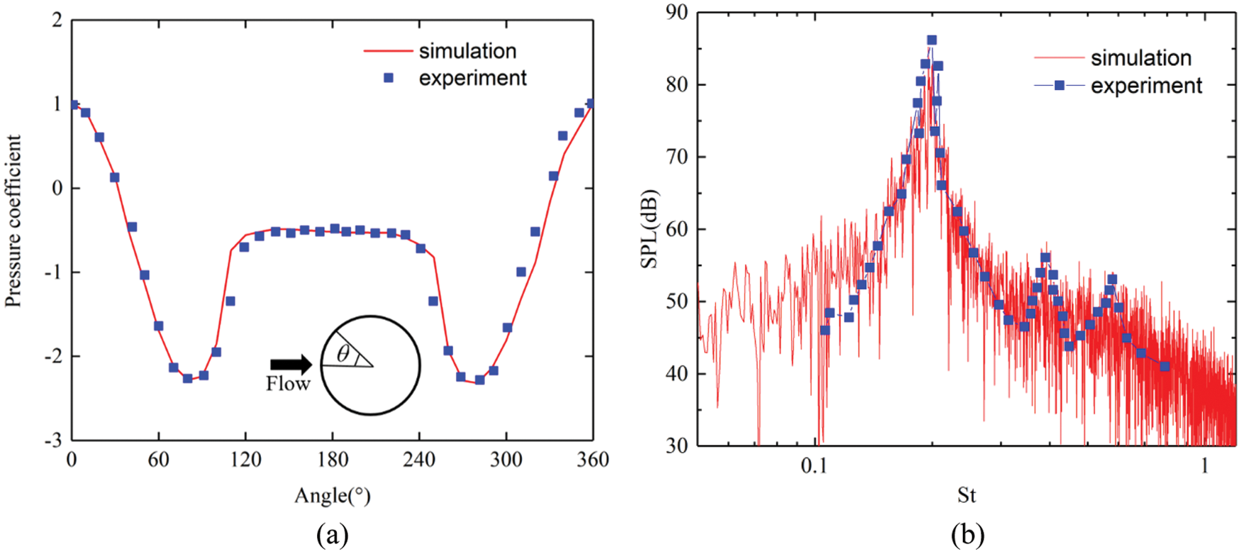
Figure 5: Comparison of simulation and experiment results (a) time-averaged pressure coefficients on the cylinder surface (b) spectrum of sound pressure level

4  Surface Aerodynamic Noise Source and Vortex Structure

4.1 Surface Aerodynamic Noise Sources

Since the value of viscous stress is small and p0 = 0, in Eq. (8), Lij ≈ pδij. Then, according to Eq. (7), the far-field aerodynamic noise of the pantograph is mainly related to the magnitude of pressure and the change rate of pressure with time on pantograph surface. Figs. 6 and 7 show the time-averaged pressure and the root mean square value of time derivative of pressure (∂p/∂t)rms on pantograph surface at the speed of 400 km/h. It can be seen from Figs. 6 and 7 that there is high positive pressure on the windward side of strip1, base frame and insulators, because the air flow stops here and kinetic energy is converted into pressure potential energy. But the pressure at these locations fluctuates weakly over time. In the wake area of the leeward side of the pantograph, energy is dissipated by vortices, so pressure here is all negative. Also, the pressure fluctuation here is very intense.

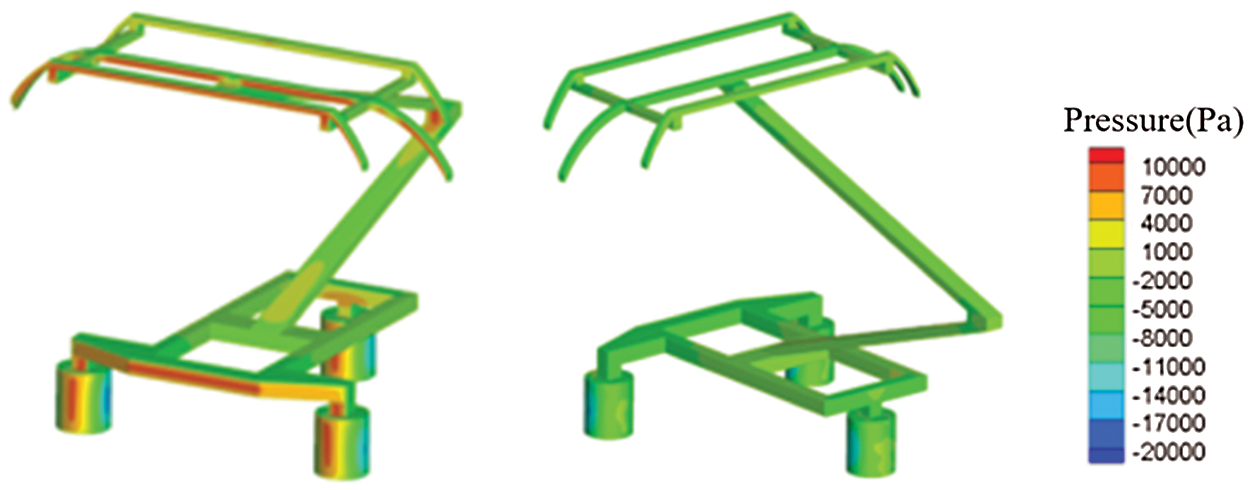
Figure 6: Pressure distribution on pantograph surface

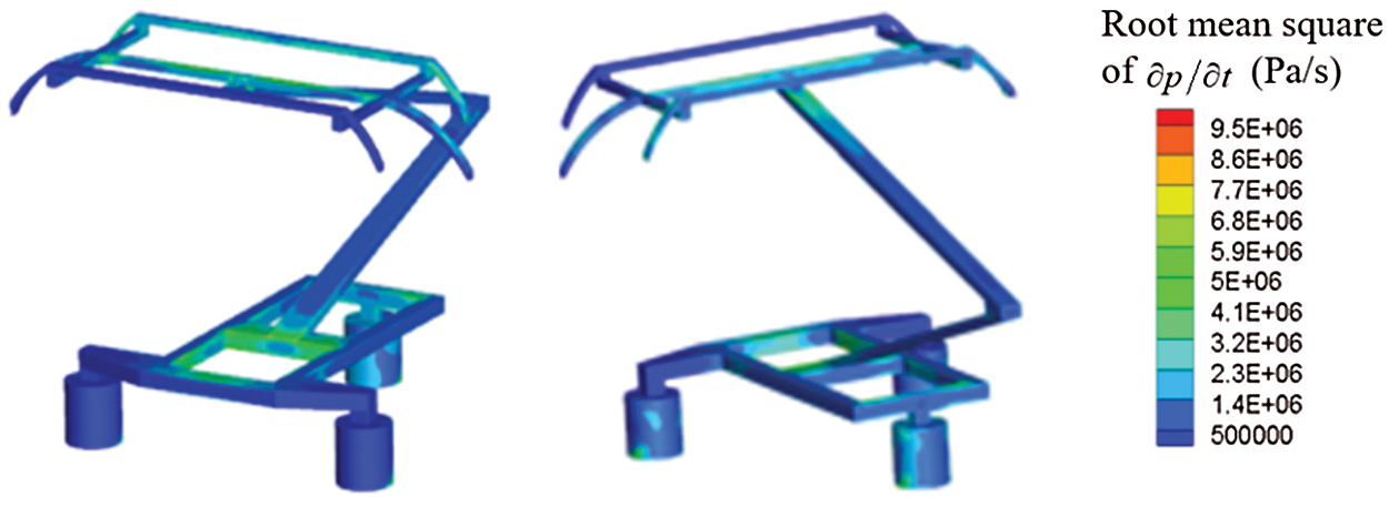
Figure 7: (∂p/∂t)rms distribution on pantograph surface

According to the results in Figs. 6 and 7, the order of magnitude of time derivative of pressure on pantograph surface is 106, that of sound velocity in air is 102, that of distance r is 101∼102, and that of fluctuating pressure on pantograph surface is 103∼104. To sum up, in the brackets of Eq. (4), the order of the first term is 102∼103, and the order of the second term is 10−1∼102. Therefore, the far-field aerodynamic noise of pantograph mainly depends on the change rate of fluctuating pressure on the pantograph surface with time and (∂p/∂t)rms can be used to characterize the aerodynamic sound source intensity on the pantograph surface. In fact, this is just as Curle pointed out: for far-field noise, when the distance between the sound source and the receiving point is far greater than the sound wave length, the first term in the bracket of Eq. (4) is the key factor [28].

According to the results of Fig. 7, the main aerodynamic sound sources on the pantograph surface include: the upper surface, windward side and leeward side of the balance arm, windward side and leeward side of the rear strip, leeward side of the base frame and insulators, upper and lower surface of the beam in the front of the base frame, and the windward side where the rear insulator and the base frame are connected with the lower arm.

4.2 Vortex Structures

Fig. 8 shows the instantaneous vortex structures of the pantograph at the speed of 400 km/h by Q criterion, which is colored by vorticity magnitude. Q is defined as:

Q=12(‖Ω‖2−‖S‖2) (9)

where ‖‖ is the second norm of the tensor, Ω is the vorticity tensor, and S is the strain rate tensor. Q criterion defines vortex as the region where the magnitude of vorticity is greater than that of shear strain rate.

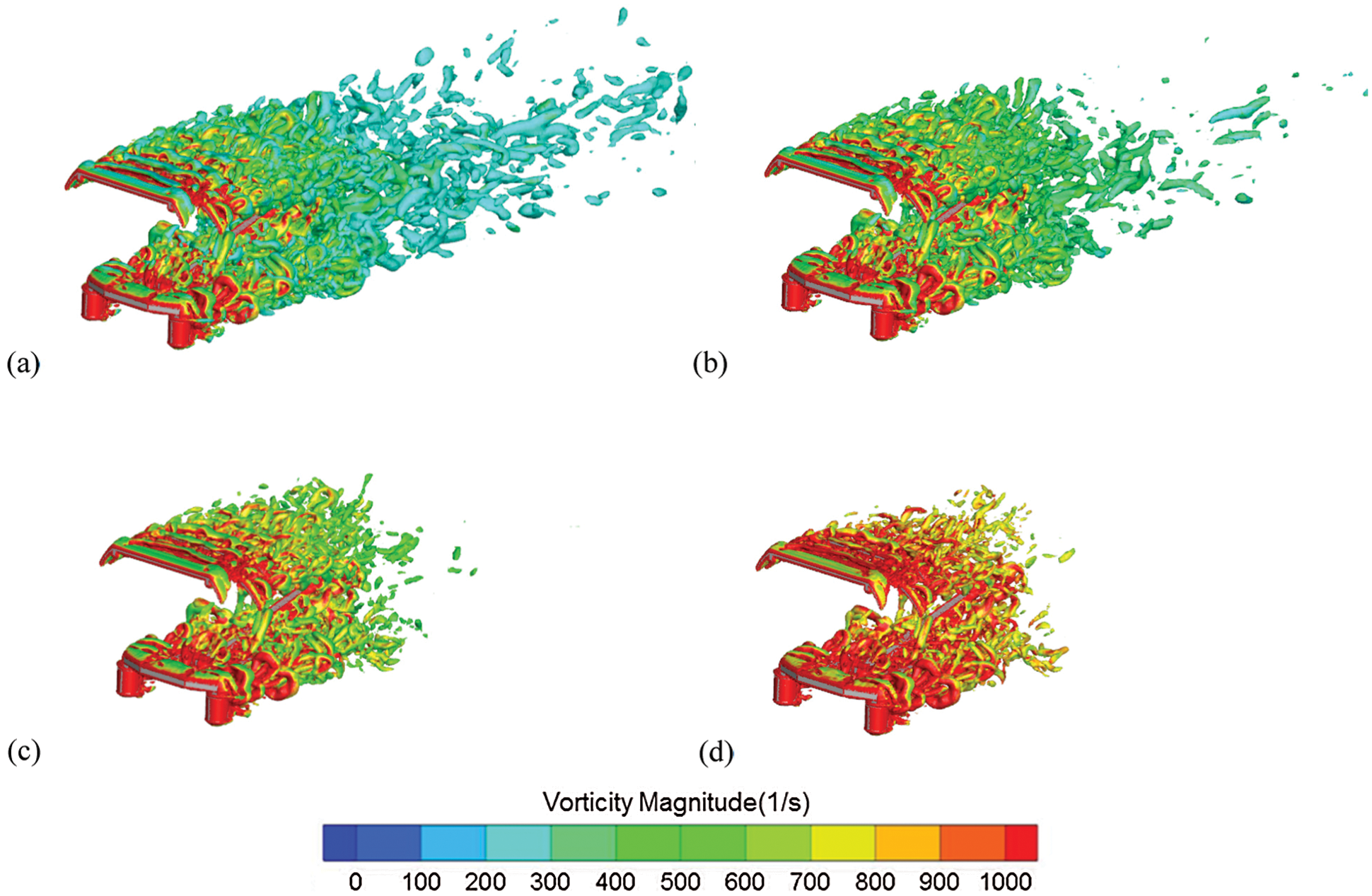
Figure 8: Instantaneous Q-isosurface (a) Q = 10000, (b) Q = 20000, (c) Q = 50000, (d) Q = 100000

It can be seen from Fig. 8 that the larger the Q is, the smaller the vortex scale and the closer it is to the pantograph. The incoming flow first splits to small foamed shape vortices on the pantograph surface, and gradually develops into a wormed-shape or hairpin-shape large scale vortices. These large scale vortices continue to move downstream. Due to the interaction between vortices, large-scale vortices gradually break into small-scale vortices. The vortices initially formed on the surface of the pantograph has large vorticity, and the vorticity decreases with the vortex moving backward away from the pantograph.

4.3 Relationship between Surface Aerodynamic Noise Sources and Vortex Structures

Fig. 9 shows the instantaneous vorticity magnitude distribution of four slices of the pantograph area at the speed of 400 km/h. They show the state of wake vortices of each component and the interaction with other components in their wake more clearly. Combining Figs. 7–9, it can be found that areas with high sound source strength can be divided into two categories. The first category is the area where the vortex sheds, such as the leeward side of balance arm, strip, base frame and insulators. The second category is the area located in the wake of the upstream components, such as the upper and lower surfaces of the front beam of the base frame (impacted by the separation vortices formed at the front edge of the front of the base frame), the upper surface and windward side of the balance arm (impacted by the separation vortices formed at the front strip), and the windward side of the rear strip (impacted by the separation vortices formed at the balance arm), the windward side of where the rear insulator and base bracket are connected with the lower arm (impacted by the separation vortices of the front beam of the base frame).

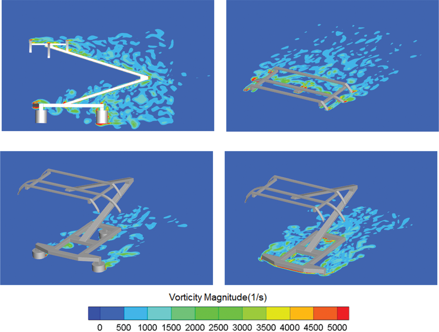
Figure 9: Instantaneous vorticity magnitude

In other words, the vortex shedding and the wake impact of upstream components will aggravate the pressure fluctuation on the pantograph surface, thus enhancing the aerodynamic noise generated by the pantograph. Therefore, in order to reduce the aerodynamic noise of pantograph, it is necessary to reduce the flow separation in the pantograph area and avoid the interaction between the wake vortices of the upstream components and the downstream components.

5  Far Field Aerodynamic Noise Characteristics

The layout of far-field noise measuring points is shown in Fig. 10, in which the measuring points p1–p13 are located on the horizontal semicircle with the center of pantograph bottom as circle center and radius of 7.5 m. q1–q7 are 7.5 m, 15 m, 25 m, 35 m, 50 m, 70 m and 100 m from the bottom center of pantograph in x-direction, and q1 is the same point with p7. All measuring points are 2 m above the ground.

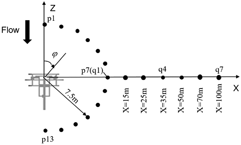
Figure 10: Measuring points layout (not to scale)

5.1 Spatial Distribution Characteristics

The directivity curves shown in Fig. 11 are obtained from the calculation results of p1–p13 measuring points. It can be seen from Fig. 11 that with the increase of radiation angle φ, the sound pressure level first decreases and then increases, and the sound pressure level on leeward side of the pantograph is significantly higher than that on windward side. That is to say, the aerodynamic noise of pantograph mainly radiates backward.

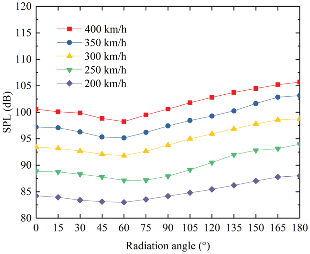
Figure 11: Directivity curves

According to the calculation results of q1–q7 measuring points, the attenuation characteristics of far-field noise of pantograph are shown in Fig. 12. It can be seen that the sound pressure level of the measuring points decreases with the increase of the distance, and the attenuation speed decrease with the increase of the transverse distance X. The relationship between the sound pressure level and logarithmic distance is approximately linear. Taking the data of speed at 400 km/h as an example, the linear function is used to fit the relationship above and Eq. (10) is obtained.

SPL(X)=−21.288lg⁡X+118.75X≥7.5R2=0.9985 (10)

It is easy to see that the sound pressure level decreases about 6.4 dB when the transverse distance is doubled. This is similar to the far-field attenuation characteristics of a point source in free field.

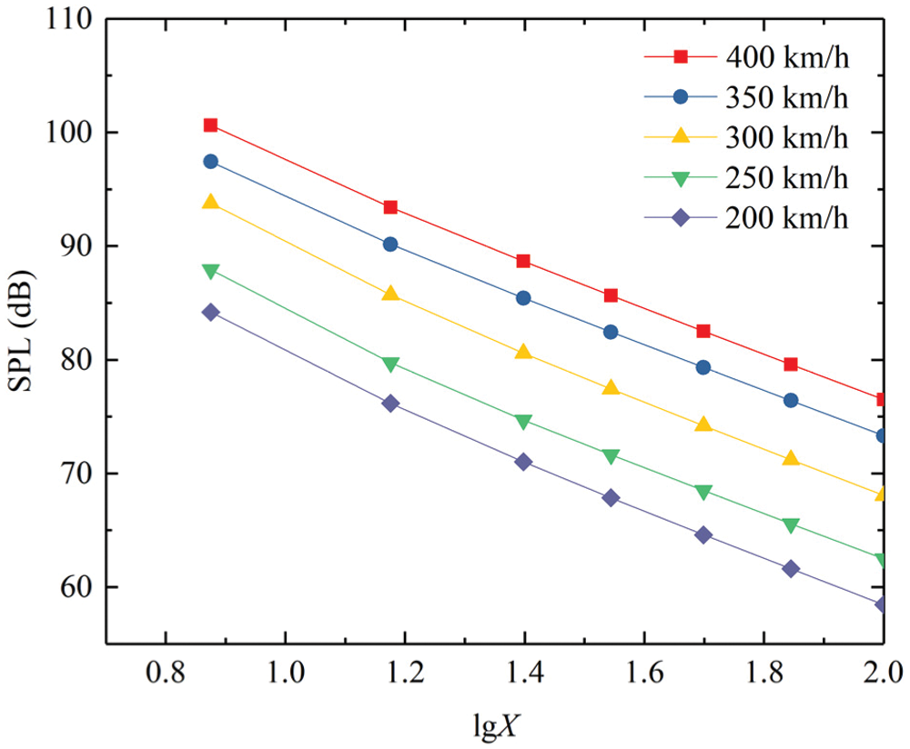
Figure 12: Attenuation characteristics

5.2 Contribution Analysis

Fig. 13 shows the contribution of the top area (strip1, strip2 and balance arm), middle area (upper arm and lower arm) and bottom area (base frame and insulators) of the pantograph to the total noise at p1–p13 measurement points at 400 km/h, which is obtained by calculating the sound pressure level the with the top area, middle area and bottom area set as sound source respectively. It can be seen from Fig. 13 that there are obvious differences in the directivity for these three areas. For top area and bottom area, the sound pressure level of the measuring points at the leeward side is higher than that at the windward side, while it is opposite for the middle area. When the radiation angle is in the range of 0° to 60°, the far-field aerodynamic noise of pantograph is mainly generated by the bottom area. With the further increase of radiation angle, the contribution of the top area and the bottom area becomes equally important and the contribution of the middle region is negligible.

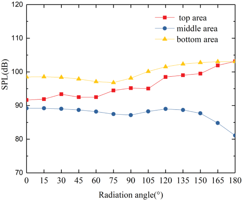
Figure 13: Contribution of top, middle and bottom areas

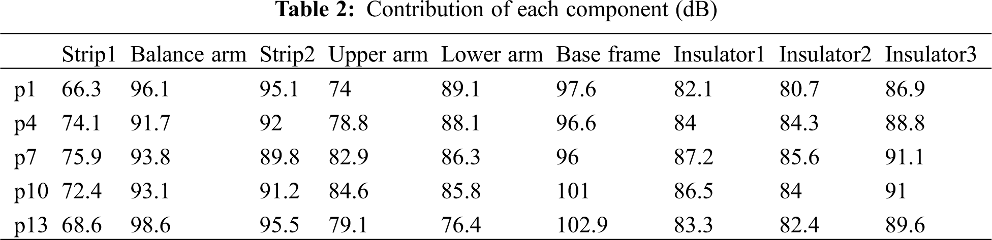
Table 2 further shows the contribution of each component to the total noise of p1, p4, p7, p10 and p13. The results in Table 2 show that the base frame, balance arm and strip2 are the key components for pantograph noise control. In addition, the contribution of the rear strip to the total noise is much greater than that of the front strip, and the contribution of the rear insulator to the total noise is also greater than that of the two front insulators, which is consistent with the analysis results in Section 4.3.

5.3 Spectrum Characteristics Analysis

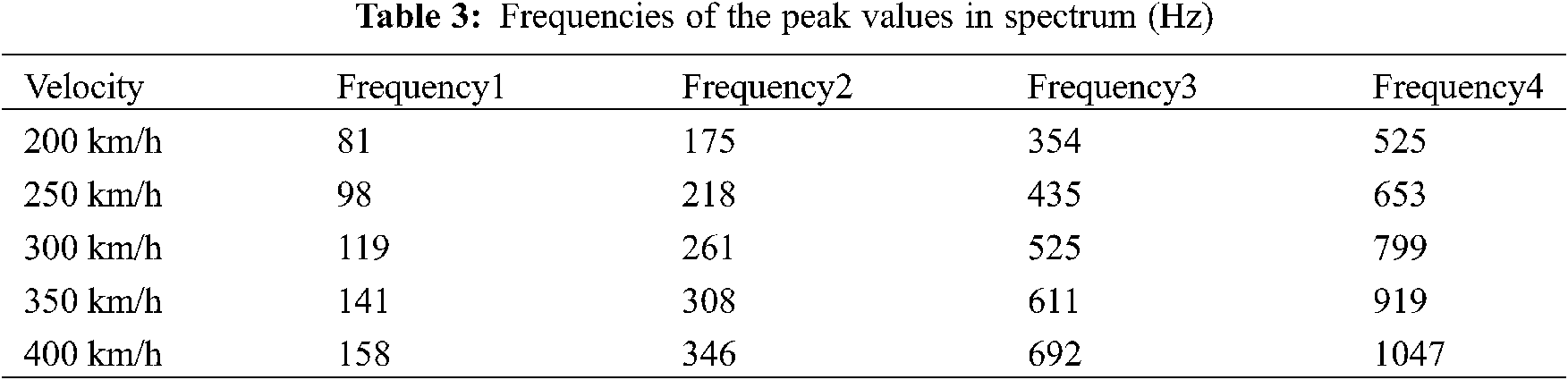
Fig. 14a shows the spectrum of sound pressure level of p1, p4, p7, p10 and p13. It can be seen from Fig. 14a that the energy of pantograph aerodynamic noise is mainly concentrated in the frequency band below 1500 Hz, and there are several peaks in the spectrum of pantograph aerodynamic noise. The peaks in the spectrum of measurement points p7, p10 and p13 are more obvious. As an example, Fig. 14b shows the spectrum of sound pressure level of p13 at different inflow velocities. It can be seen from Fig. 14b that the peaks moves to high frequency with the increase of inflow velocity, which conforms to Strouhal criterion. The peak frequencies at different inflow velocities are given in Table 3.

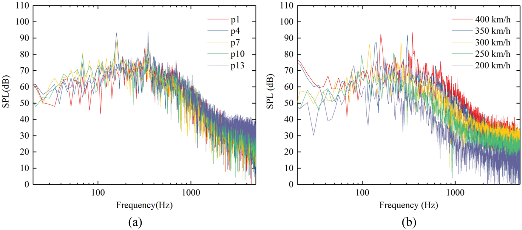
Figure 14: Spectrum of sound pressure (a) spectrum of SPL at different radiation angles (b) spectrum of SPL at different inflow velocities (p13)

Since p7 is the measuring point located at the track side that usually used for noise evaluation, the sound pressure level at p13 is the highest and the peaks in its spectrum is the most obvious, p7 and p13 are taken as examples to further analyze the source of peaks in the spectrum of pantograph aerodynamic noise. The spectrum of p7 and p13 is calculated with each component as the sound source at the inflow velocity of 400 km/h, as shown in Figs. 15 and 16. The analysis of the spectrum of each component shows that although the spectrum of most components has peak values, when the spectrum of each component is superimposed together, some peaks with smaller amplitude will be covered up. Therefore, the total spectrum does not show all the peaks in the spectrum of components. The spectrum of strip1, strip2 and balance arm corresponds to the peak at 346 Hz, 692 Hz and 1047 Hz in p13 spectrum, which is the frequency and harmonic frequency of periodic vortex shedding at strips and balance arm. However, the amplitude of the sound pressure level of the balance arm and strip2 at these frequencies is significantly greater than that of the strip1, which is mainly related to the interaction between the wake of the strip1 and the balance arm and the strip2 according to the analysis in 4.2 and 4.3. However, in the spectrum of p7, only two peaks at 158 Hz and 346 Hz are clearly visible, while the peaks the harmonic frequency at 692 Hz and 1047 Hz are not as clear as p13. This is mainly related to the directivity of the sound source. The peak in the spectrum of the base frame corresponds to the peak value at 158 Hz in the spectrum of p7 and p13, and this peak comes from the vortex shedding at the front beam of the base frame. For p13, the peaks at 158 Hz and 346 Hz can also be observed in the spectrum of the upper and lower arms, but their values are about 20 dB lower than the corresponding peaks of the balance arm, strip 2 and base frame. Obviously, the peaks at 158 Hz and 346 Hz in the spectrum of the upper and lower arms are not caused by the vortex shedding of the upper and lower arms themselves, but by the interaction between the wake vortices in the base frame and panhead area and the upper and lower arms. The peak at 158 Hz can also be observed in the spectrum of the insulators at p13, which is the same as that in the spectrum of upper and lower arms. This peak is not caused by the vortex shedding of the insulators themself, but by the interaction between the wake of the base frame and the insulators. In conclusion, in the spectrum of p7 and p13, the peak at 158 Hz is mainly contributed by the base frame and the peak at 346 Hz is mainly contributed by the balance arm and strip2. In the spectrum of p13, two peaks at 692 Hz and 1047 Hz can also be observed, which are the harmonic frequencies of 346 Hz.

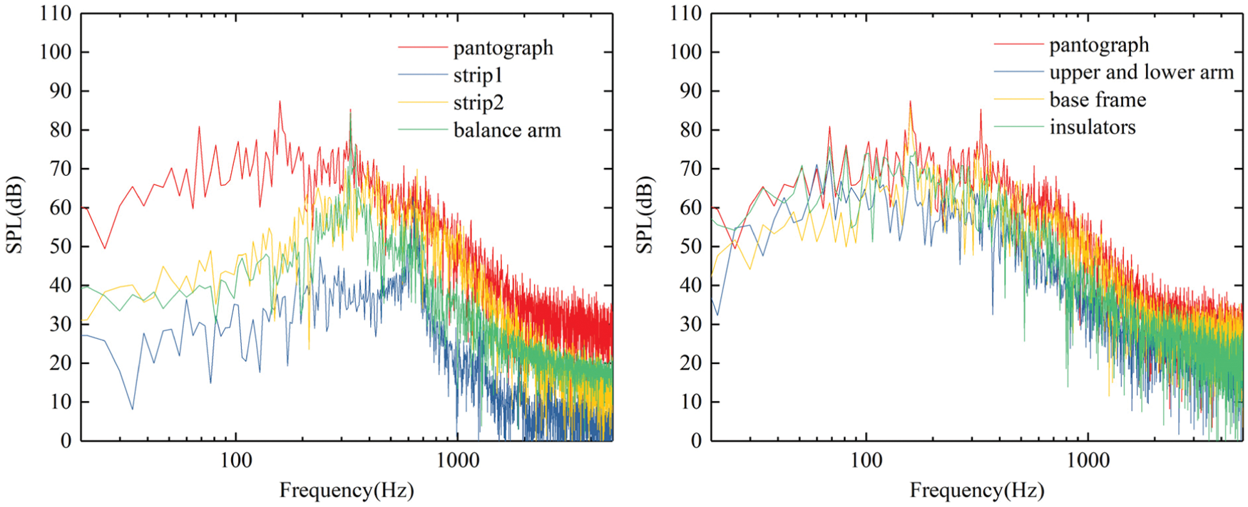
Figure 15: The spectrum of each component at p7

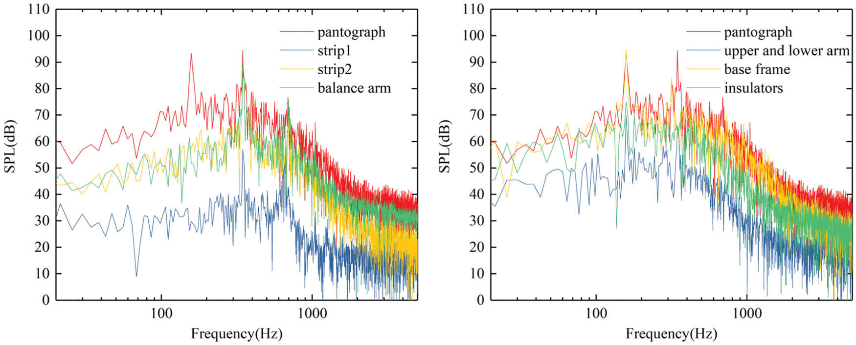
Figure 16: The spectrum of each component at p13

It can also be found from Figs. 15 and 16 that for the broadband noise without peak value, the base fame makes great contribution to the whole frequency band, the insulators mainly contribute to the noise below 200 Hz, while the strips and the balance arm mainly contributes to the noise above 200 Hz. Compared with p13, the contribution of upper and lower arm to p7 below 200 Hz is more significant.

5.4 Inflow Velocity Dependent Regularity

Fig. 17a shows the relationship between linear weighted sound pressure level and inflow velocity of p3, p7 and p13. It can be seen from Fig. 17a that the linear weighted sound pressure level of pantograph far-field noise is approximately linear with the logarithm of inflow velocity, and the scale coefficient is about 50 to 60. This is approximately in accordance with the law of the increase of the aerodynamic noise of the dipole source with the inflow velocity.

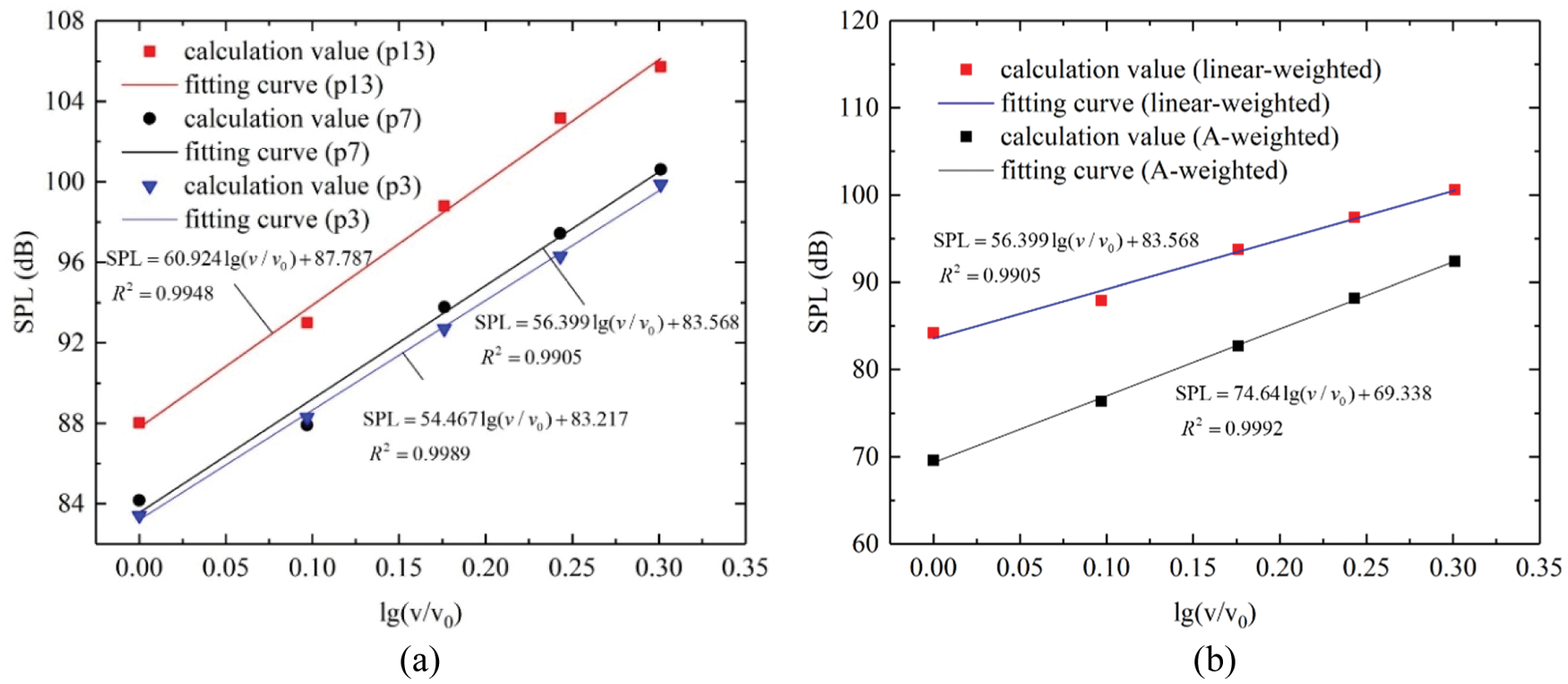
Figure 17: Inflow velocity dependent regularity (a) linear weighted results (b) comparison of linear- weighted and A-weighted results

In high-speed railway engineering, A-weighted sound pressure level is usually used to evaluate the far-field noise. Fig. 17b further shows the growth law of A-weighted sound pressure level with speed at p7. It can be seen from Fig. 17b that the A-weighted sound pressure level is also approximately linear with the logarithm of the inflow velocity. However, due to that the main frequency of the aerodynamic noise of the pantograph moves to the high frequency with the increase of the inflow velocity and the attenuation after weighting decreases, the A-weighted sound pressure level increases faster with the inflow velocity.

6  Conclusions

In this study, a LES/FW-H hybrid method is used to investigate the aerodynamic noise characteristics of a simplified double-strip pantograph. The location of the main sound source on the pantograph surface is determined by the CFD results. The vortex structures in the pantograph flow field are studied based on Q-criterion. The relationship between them is discussed to reveal the generation mechanism of pantograph aerodynamic noise and provide guidance for noise reduction. The characteristics of far-field aerodynamic noise are also studied.

The results show that the aerodynamic noise of pantograph surface is mainly related to the change rate of the surface pressure with time on pantograph surface. (∂p/∂t)rms can be used as an index to characterize the sound source intensity on pantograph surface and determine the main source location.

The aerodynamic sound source on the surface of the pantograph is closely related to the vortex structures of the pantograph. The pressure fluctuates violently where the vortex sheds or impacted by the wake of the upstream components and these areas are the main sound sources location. Therefore, in order to control the aerodynamic noise of pantograph, it is necessary to reduce the flow separation on the surface of pantograph and avoid the interference of the upstream components wake on the downstream components.

The aerodynamic noise of pantograph mainly radiates backward. When the transverse distance is greater than 5 m, it’s attenuation characteristics is similar to the far field attenuation characteristics of a point source in free field. The far-field aerodynamic noise energy of pantograph is mainly concentrated in the frequency band below 1500 Hz. The peak value of the frequency spectrum is mainly generated by the base frame, balance arm and the rear strip. They are also the components that contribute the most to the far-field aerodynamic noise. The linear weighted sound pressure level and A-weighted sound pressure level of the far-field aerodynamic are approximately linear with the logarithm of the inflow velocity. For the linear weighted sound pressure level, the proportion coefficient is about 50∼60, which is similar to the velocity dependence regularity of a dipole source. For A-weighted sound pressure level, as the main frequencies of the pantograph aerodynamic noise move to high frequency band with the increase of inflow velocity and the attenuation after weighting decreases, so it increases faster with the inflow velocity.

Funding Statement: This work is funded by National key R&D Program China (2016YFE0205200) and National Natural Foundation of China (U1834201).

Conflicts of Interest: The authors declare that they have no conflicts of interest to report regarding the present study

This work is licensed under a Creative Commons Attribution 4.0 International License, which permits unrestricted use, distribution, and reproduction in any medium, provided the original work is properly cited.