| Fluid Dynamics & Materials Processing |
DOI: 10.32604/fdmp.2021.016618
ARTICLE
Numerical Study on the Blade Channel Vorticity in a Francis Turbine
Yellow River Conservancy Technical Institute, Kaifeng, 475003, China
*Corresponding Author: Zhiqi Zhou. Email: zhiwomu5@163.com
Received: 12 March 2021; Accepted: 12 July 2021
Abstract: A relevant way to promote the sustainable development of energy is to use hydropower. Related systems heavily rely on the use of turbines, which require careful analysis and optimization. In the present study a mixed experimental-numerical approach is implemented to investigate the related mixed water flow. In particular, particle image velocimetry (PIV) is initially used to verify the effectiveness of the numerical model. Then numerical results are produced for various conditions. It is shown that an increase in the guide vane opening can reduce the extension of the region where the fluid velocity is 0 at the inlet of the runner blade, i.e., it can counteract the generation of the channel vortex; an increase in the guide vane opening also contributes to mitigate the pressure acting on the runner blade; no matter what the working conditions are, the surface pressure is usually higher than that on the suction surface, and there is a cliff-like drop of pressure at the tail of the blade, which indicates that the runner blade tail is more prone to develop backflow.
Keywords: Hydropower; Francis turbine; numerical simulation; channel vortex
At present, electric power has been a widely used secondary energy, and thermal power generation is its most frequent production form; however, a massive quantity of fossil fuels consumes in the process of generating power with thermal power [1]. Hydropower [2] is a kind of clean energy, and its basic principle is to drive the rotor in a generator to rotate and achieve the effect of magnetic generation by driving the turbine with the flowing water generated by the altitude difference of terrain. It is seen from the basic principle of hydropower that the turbine used to drive the generator rotor is the core element [3]. During use, the adjacent blades of a rotor machine will induce the channel vortex, which leads to the uneven pressure on the blades, and the vibration and distortion generate under the continuous water flow impact. The vibration and distortion accelerate the consumption of blade life and seriously affect the safety of the whole hydropower system. Biswas et al. [4] analyzed the turbine with the finite element method and found that the static pressure at the middle surface usually decreased from the outer wall to the volute outlet. Guo et al. [5] have systematically studied the blade channel vortex phenomenon of the Francis turbine from aspects of hydraulic design, experiment, and numerical calculation. The results showed that the channel vortex phenomenon of the Francis turbine was its inherent characteristic under the small flow condition and the turning point of the channel vortex inception curve appeared in the low unit speed region. Miao et al. [6] analyzed the energy conversion effect of the volute of a centrifugal pump with computational fluid dynamics. The outcomes confirmed that the conversion of dynamic pressure energy and static pressure energy mainly depended on the reduction of the flow area in the contraction section of the volute, and friction loss also played a vital role in the spiral section. In the previous related studies, the internal hydraulic performance of the water turbine was studied by the numerical calculation. However, due to the relatively complex internal structure of the Francis turbine, different parts are studied separately rather than as a whole. Among the two related studies mentioned above, the former mainly studies the static pressure distribution on the inner wall of the water flow inside the water turbine, while the latter studies the velocity distribution of the blade vortex in the water turbine on the passage. In this study, the internal flow of the Francis turbine was calculated by numerical simulation, and the numerical model was verified by the actual water turbine model. The novelties of this paper are that the internal flow of the turbine was studied by the numerical simulation, and the traditional standard
2 Introduction of Francis Turbine
For hydroelectric power generation, water turbines are the core equipment. The Francis turbine is currently the most widely used turbine. The Francis turbine is a reaction turbines, and part of its structure is shown in Fig. 1. When the Francis turbine is working, the water will flow in radially from all sides of the runner blades and then flow out in the axial direction as much as possible. The Francis turbine is relatively compact in basic structure and has high rotation efficiency. As the water flows in from all sides of the runner, it can adapt to a wider water head. The basic structure of a Francis turbine includes a volute, a seat ring, a water guide, a top cover, a runner, a main shaft, etc. The runner and volute [7] are shown in Fig. 1.
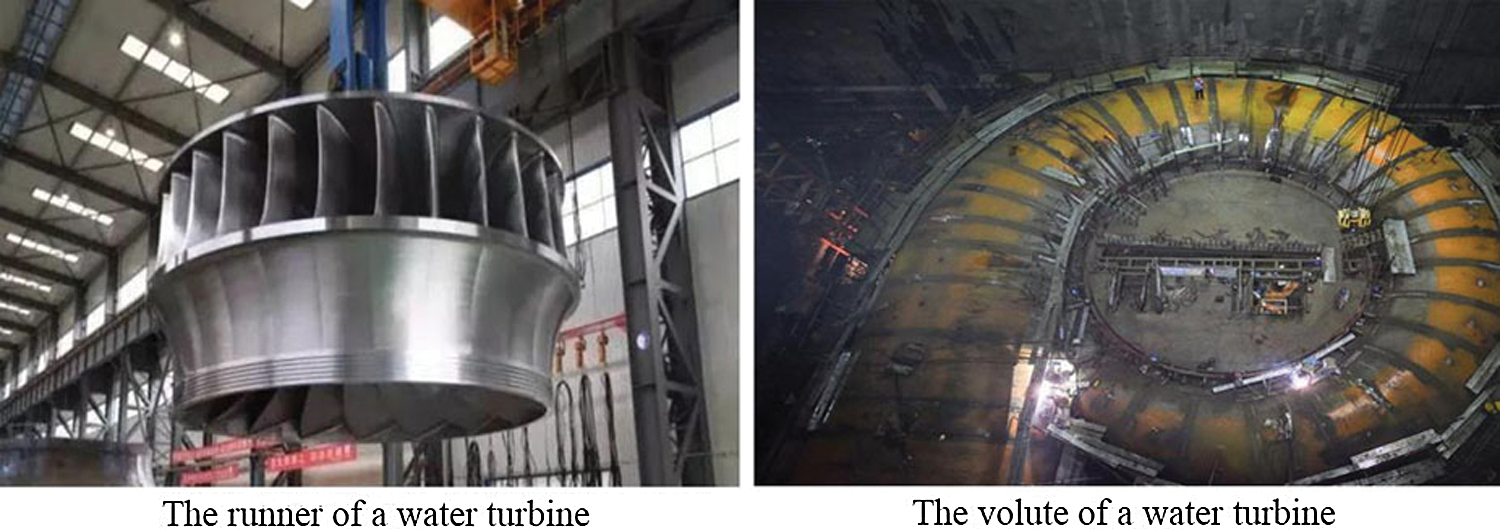
Figure 1: Some pictures of a Francis turbine
3 Numerical Calculation of Flow Field
In order to ensure the authenticity of the research results, the ideal condition is to directly test the blade channel vortex of the inner runner of the Francis turbine [8]; however, due to the large scale of the actual Francis turbine, the cost of the experiment is too high. Therefore, the Francis turbine model reduced in equal proportion will be used for the experiment [9]. The Francis turbine model is similar to the actual Francis turbine in geometry, motion, and power, which plays an important role in the related research of the Francis turbine. However, it is difficult to observe the cavitation phenomenon caused by the blade channel vortex because of the complex structure of both the actual turbine and the turbine model. Simply speaking, the measurement is difficult. Also, the adjustment of the experimental conditions is not flexible enough, and the experimental cost is high.
With the help of computer and numerical simulation technology [10], it is more convenient and low-cost to study the blade channel vortex of the Francis turbine and can adjust experimental conditions more easily and quickly when studying the influence of different working conditions on the hydraulic turbine.
The governing equations for numerical simulation follow the mass conservation equation [11] and momentum conservation (N-S equation) [12], and the equations are:
where
When performing numerical simulation on the internal fluid flow of the Francis turbine [14] with Eq. (2), it is necessary to solve the equation set before obtaining the required fluid parameters. When the numerical simulation is performed on the fluid using the equation set in Eq. (2), it is necessary to ensure that the equations are closed; therefore, it is necessary to use an appropriate turbulence model [15] to solve the equation set. The
where
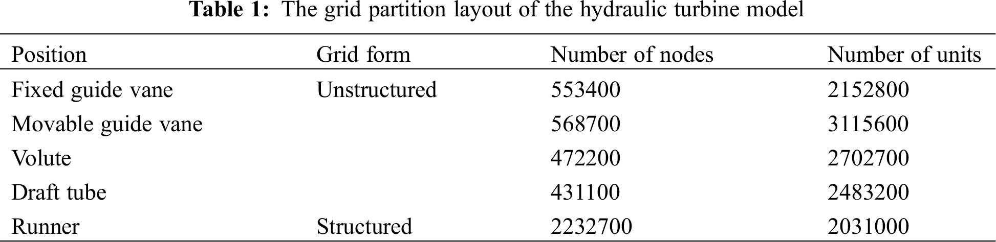
The basic model of the Francis turbine is shown in Fig. 2. The basic parameters of the hydraulic turbine are as follows: The highest water head was 150; the maximum flow was 1.5 m3/s; the maximum rotational speed of the runner was 2600 r/min; the maximum power of the dynamometer was 600 kW; the runner diameter of the hydraulic turbine was 500 mm; the number of fixed guide vanes was 24; the number of movable guide vanes was 26; the number of runner blades was 16. After the model was implemented, grid partition was performed on the hydraulic turbine model using the grid generation software [16], and the final partition scheme is shown in Tab. 1.
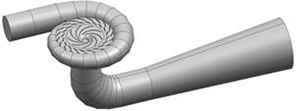
Figure 2: The basic model of a Francis turbine
The numerical simulation steps of the Francis turbine are as follows:
1. A simulation model of the Francis turbine was implemented, as shown in Fig. 2. The basic parameters of the models are as follows. The largest height of the water head was 150 m. The maximum flow rate was 1.5 m3/s. The maximum rotational speed of the runner was 2600 r/min. The maximum power of the dynamometer was 600 kW. The diameter of the runner was 500 mm. The number of the fixed guide vanes was 24. The number of the movable guide vanes was 26. The number of runner blades was 16.
2. Meshing was performed on the simulation model of the Francis turbine. In this study, ANSYS ICED was used for meshing. Before meshing, the mesh irrelevance test was carried out. The main indicators of the irrelevance test were the efficiency and output power under the designed working condition. Under the same working condition (the opening of movable guide vanes: 18°; the unit rotational speed of the runner: 75 r/min; the unit flow: 500 L/s), the results of the mesh irrelevance test are shown in Fig. 3. It was seen from Fig. 3 that the efficiency and output power of the water turbine obtained by the numerical calculation model increased gradually and then tended to be stable with the increase of the number of grid points, and the two indicators of the Francis turbine kept stable after the number of grid points became 2 × 10⁶; therefore, the final mesh number of every structure in every Francis turbine is as described in Tab. 1.
3. The numerical simulation was performed on the simulation model after meshing. The governing equation was needed in the process of operating the fluid dynamics software. The governing equations used in the calculation process included the mass conservation equation and momentum conservation equation. As the fluid for numerical simulation was water in this study, which was regarded as incompressible, the N-S equation was adopted, whose formula has been shown in Eq. (1). When the mass conservation equation and the N-S equation were solved, a proper turbulence model should be selected to ensure the closure of the equation. In this study, the RNG
4. In the numerical calculation of the fluid flow inside the turbine, the numerical model was further restricted. The boundary conditions of the numerical model were set in the calculation process. The first was the inlet boundary. The specific settings of the inlet boundary are as follows: The fluid flow property was set as subsonic velocity; the fluid inflow computational domain adopted the standard speed; the turbulent kinetic energy coefficient was set as 5%. Next was the outlet boundary. The specific settings of the outlet boundary are as follows. The outlet of the computational domain was the opening boundary type. The fluid outflow calculation domain was set as the opening pressure and direction, and the other conditions were consistent with the inlet calculation domain. Next was the wall boundary condition. The wall boundary was non-slip. The area around the wall adopted the standard wall function. The last was the setting of the dynamic and static interface in the process of fluid flow. The runner area of the turbine was calculated under the rotating reference system, and the flow area of other static parts was calculated under the static reference system. Frozen rotor was used for coupling between the rotating area and the static area to realize the transfer of the flowing data between dynamic and static parts.
5. Discrete format setting. The numerical model was discretized by the finite volume method. The discrete format was the first-order upwind style; the step size was consistent with the interval between frames of the camera in the PIV experiment, which facilitated the comparison in the verification experiment. In the numerical calculation, the convergence condition for determining the termination of the iterative simulation was that the residual value [17] reached 0.0001.
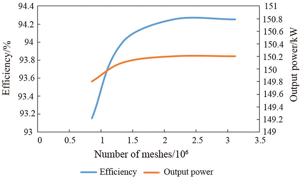
Figure 3: The mesh irrelevance test
4.2 Numerical Simulation Project
In this study, the working conditions used in the numerical simulation of the hydraulic turbine are shown in Tab. 2. In the two conditions, except the guide vane opening, the unit speed, speed, and unit flow were the same.
After the model meshing, boundary setting, and working condition setting, numerical simulation was carried out on the fluid in the hydraulic turbine to output the required results. In order to ensure the accuracy of the numerical simulation results of the model, the actual turbine model was tested by PIV technology [18] to verify the effectiveness of the numerical model. The basic principle of PIV technology for fluid flow field testing is as follows: Tracer particles are added to the fluid to be tested. Tracer particles not only need to ensure that the material is safe and the particle size is small enough but also need to ensure that the density is as close as possible to the fluid density. The fluid is irradiated by laser. The flow field is visualized because of the scattering effect of tracer particles. Images are taken by a camera to analyze the flow field law.
The steps of testing the actual turbine model with PIV technology are as follows: (1) The hydraulic turbine model was filled with water, and the PIV test system was tested to ensure that it met the test requirements. (2) Tracer particles were put into the model, and hollow glass beads were used as tracer particles in this study (the reason for using the hollow glass bead was that its density could be adjusted to be close to the density of water body and it can scatter the incident light better); (3) The laser emitter was turned on, the incident angle and height were adjusted to make the laser irradiate at 50% of the height of the runner blade, and the camera was turned on to collect the flow image of tracer particles in the flow field from the observation window of the hydraulic turbine model. (4) The hydraulic turbine model was started, the hydraulic turbine was adjusted according to the set working conditions, and the camera collected the corresponding flow field images in the process of the experiment. (5) The image of the flow field was calculated using a computer to analyze the flow law of the flow field in the hydraulic turbine.
In this study, the main purpose of testing the actual model of the hydraulic turbine with PIV technology is to test the accuracy of the numerical model of the hydraulic turbine; therefore, the working conditions used in the experiment process were consistent with those in the numerical simulation, or the working conditions used in the numerical simulation came from the actual model test. The difference between the actual model and the numerical model was compared by the hydraulic efficiency and head of the hydraulic turbine to judge the effectiveness of the numerical model. The calculation formula of hydraulic efficiency [19] is:
where
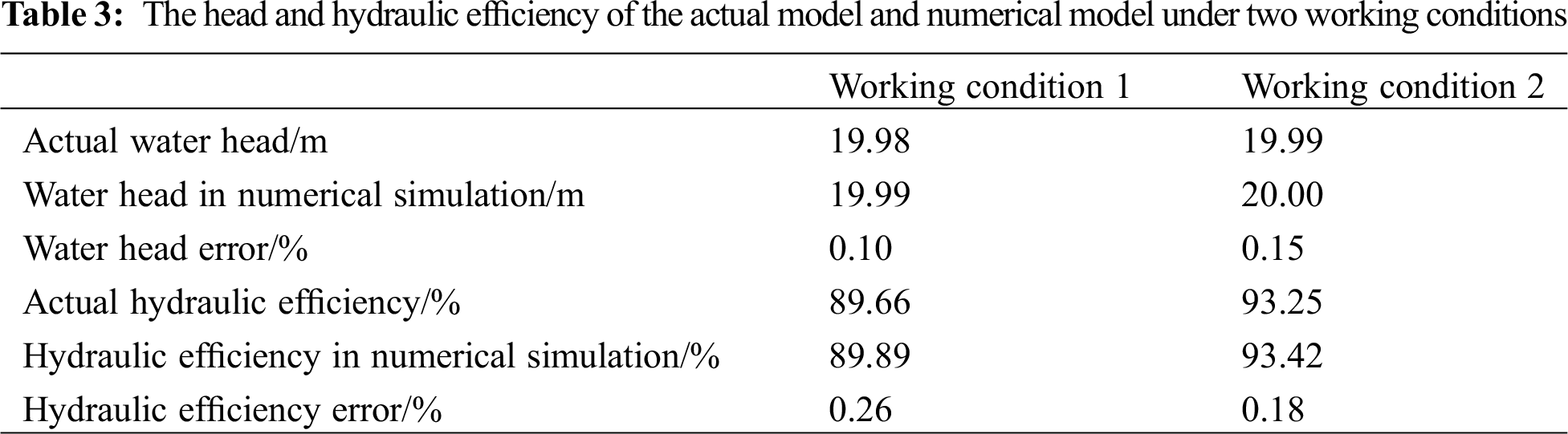
The validity of the hydraulic turbine numerical model was verified by the actual turbine model. The test results of the head and hydraulic efficiency of the two hydraulic turbines are shown in Tab. 3. It was seen from Tab. 3 that the water head used in the two working conditions was about 20 m, in which the head error under working condition 1 was 0.10%, and that under working condition 2 was 0.15%; in terms of hydraulic efficiency, there was a relatively obvious difference between the two working conditions, in which the hydraulic efficiency error under working condition 1 was 0.26%, and that under working condition 2 was 0.18%. Through the comparison in Tab. 3, it was seen that the error between the results of the simulated calculation by the numerical model and the actual model results was small, and the numerical simulation results could be effectively used for analyzing the internal flow field of the hydraulic turbine.
The numerical model of the hydraulic turbine was verified by the actual hydraulic turbine model, and the fluid under two working conditions was numerically simulated. As this study mainly analyzed the blade channel vortex generated at the runner in the hydraulic turbine, the water flow velocity distribution at 90% height of the runner blade under two working conditions was shown here, as shown in Fig. 4. It was seen from Fig. 4 that the flow velocity distribution at 90% height of the runner blade of the hydraulic turbine was quite close under the two guide vane openings: there was a partial region where the fluid flow velocity was 0 at the inlet of the runner blade, the fluid flow velocity gradually increased as the flow surface gradually approached the lower ring region in the center, and the region with a fluid flow velocity of 0 was generated by the blade channel vortex according to the numerical calculation. By comparing the velocity distribution diagrams of two working conditions, it was found that the area where the flow velocity at the runner blade inlet was 0 decreased, and the overall velocity was more balanced when the guide vane opening increased, i.e., the increase of the guide vane opening could reduce the generation of blade channel vortex.
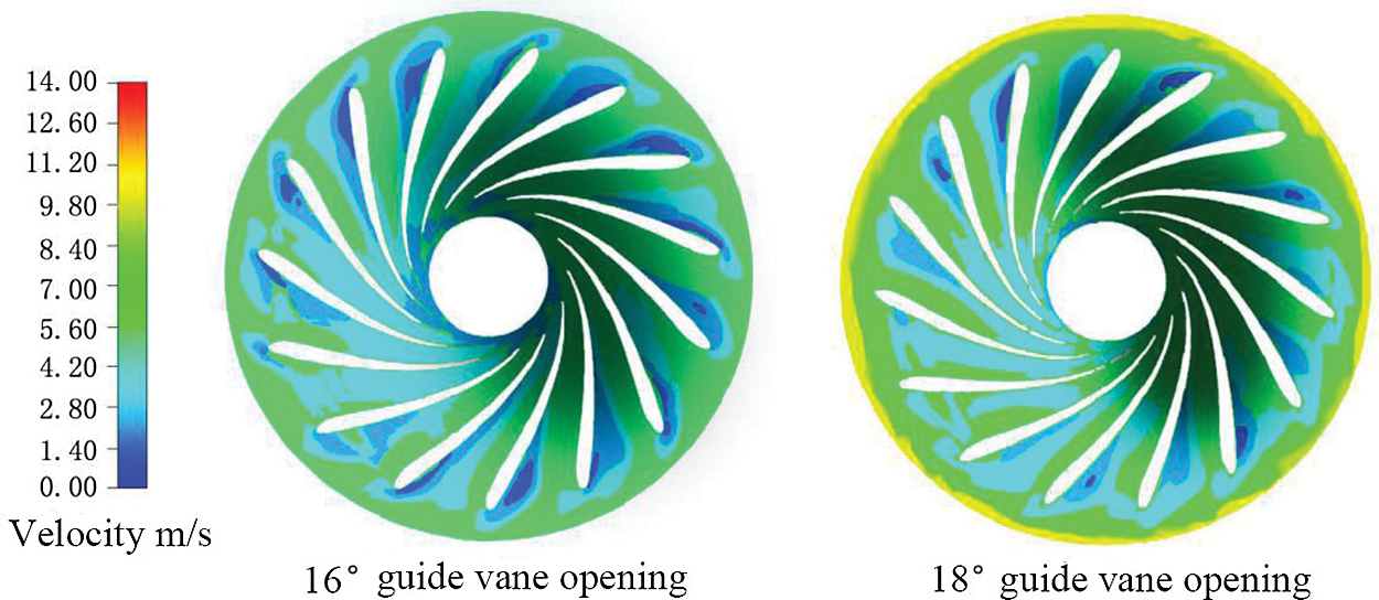
Figure 4: The water velocity distribution at 90% height of the runner blade of the hydraulic turbine under two working conditions
Fig. 5 shows the pressure distribution curve of suction and pressure surface at 90% height of the runner blade obtained by numerical calculation. It was seen from Fig. 5 that the pressure distribution trend of suction surface and pressure surface at 90% height of runner blade was similar under the two working conditions: the pressure values decreased from the downstream inlet to the downstream outlet, the pressure change of the blade pressure surface was larger than that of the suction surface, and the pressure on the blade surface also reduced with the increase of the guide vane opening. The comparison of the pressure distribution on both sides of the runner blade in the same working condition showed that the surface pressure on the pressure surface was higher than that on the suction surface, and there was a cliff-like drop in the pressure at the tail of the blade, i.e., the backflow phenomenon was more likely to appear at the tail of the runner blade.
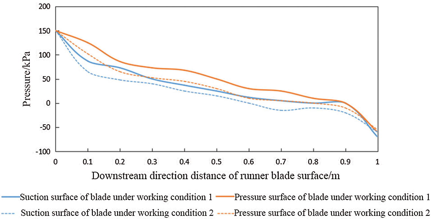
Figure 5: Surface pressure distribution curve of the runner blade of the hydraulic turbine at 90% height under two working conditions
As a kind of sustainable energy, hydropower has been widely used. The hydraulic turbine is the core equipment of hydropower generation. The flowing water flows into the turbine runner along the inlet pipe and drives the runner to rotate so that the generator rotor rotates in the magnetic field and generates electricity. However, in the process of using the hydraulic turbine, the blades of the runner will bear the pressure due to the impact of the water flow, and the adjacent blades will induce the blade channel vortex, resulting in the uneven pressure on the blades, and the vibration and distortion generate under the continuous impact of the water flow.
Due to the huge power of hydropower generation, the size of the hydraulic turbine is large. The component structure is not transparent. Even if the model that is reduced in proportion is used for the experiment, it is difficult to observe and analyze the internal flow field completely. The maturity of computer technology provides a more convenient means for the analysis of the internal flow field of the hydraulic turbine, i.e., simulate the fluid flow field with computers to analyze the internal flow field more completely. In this study, the blade channel vortex of the hydraulic turbine was analyzed by the numerical simulation method. First of all, before analyzing the flow field with the numerical model, the validity of the numerical model was verified by the actual hydraulic turbine model in aspects of the head and hydraulic efficiency. The verification results are as shown above. The error between the results of the numerical model and the actual model was small, indicating that the numerical model could effectively simulate the fluid flow field. The numerical calculation was performed on two working conditions with different guide vane openings using the numerical model. The velocity distribution and blade surface pressure distribution at 90% height of the runner blade under two working conditions are shown above. The numerical calculation results showed that the region where the flow velocity was 0 at the inlet of the runner blade decreased with the increase of the guide vane opening, i.e., the blade channel vortex decreased; the pressure distribution on the surface of the runner blade showed that the pressure on the blade surface decreased with the increase of the guide vane opening.
The reason for the above results is as follows. The angle of attack formed by the direction of flow velocity at the runner inlet and the direction of the inlet edge was negative, which made the water unable to flow fully fit the blade, i.e., flow separation, and the secondary flow occurred when the water body after the flow separation contacted with the blade surface again. The flow separation and secondary flow induced the blade channel vortex. The flow velocity in the region where the vortex was located was about 0. In numerical calculation, the fluid flow velocity distribution diagram showed that the blade channel vortex, which made the flow velocity zero, generated on the pressure surface of the runner blade. The existence of the blade channel vortex squeezes the water in the runner channel and accelerates the flow velocity on the suction surface of the blade. The difference in the flow velocity on both sides of the runner blade led to different pressures on the blade surface. The existence of the blade channel vortex led to uneven flow velocity on both sides and uneven pressure on the blade surface, which was also the reason for the downward trend of the pressure distribution curve.
In this study, the flow field in the Francis turbine was calculated by numerical simulation, and the numerical model was verified by the actual water turbine model. The final results are as follows: (1) the head and hydraulic efficiency of the actual turbine model measured by PIV technology had a small error with the results calculated by the numerical model, which verified the effectiveness of the numerical model; (2) when the opening of the guide vane increased, the blade channel vortex at the inlet of the runner blade decreased, and the area with a flow velocity of 0 also decreased; (3) when the opening of the guide vane increased, the pressure on the runner blade decreased, the pressure on the pressure surface of the blade was higher than that on the suction surface, and the pressure at the tail of the blade dropped precipitously. This paper studied the influence of guide vane opening of the runner in a water turbine on internal vane vortex through analyzing the internal fluid inside the Francis turbine using the numerical simulation method and provided an effective reference for improving the working efficiency of the Francis turbine.
Funding Statement: The author received no specific funding for this study.
Conflicts of Interest: The author declares that he has no conflicts of interest to report regarding the present study.
1. Murgan, I., Vasile, G., Ioana, C., Barre, S., Ronco, T. L. (2017). Hydraulic turbine vortex detection and visualization using strain gauge sensor. IEEE Sensors Letters, 1(5), 1–4. [Google Scholar]
2. Nishi, Y., Sato, G., Shiohara, D., Inagaki, T., Kikuchi, N. (2019). A study of the flow field of an axial flow hydraulic turbine with a collection device in an open channel. Renewable Energy, 130, 1036–1048. [Google Scholar]
3. Kurir, V. I. (2019). Towards the development of an impeller with splitters for a radial-axial hydraulic turbine. Hydrotechnical Construction, 53(1), 62–64. [Google Scholar]
4. Biswas, G., Eswaran, V., Ghai, G., Gupta, A. (2015). A numerical study on flow through the spiral casing of a hydraulic turbine. International Journal for Numerical Methods in Fluids, 28(1), 143–156. [Google Scholar]
5. Guo, P. C., Wang, Z. N., Luo, X. Q., Wang, Y. L., Zuo, J. L. (2016). Flow characteristics on the blade channel vortex in the Francis turbine. IOP Conference Series Materials Science and Engineering, 129(1), 012038. [Google Scholar]
6. Hisasue, N., Takehara, K., Shindou, S., Takano, Y. (2016). Experimental study on hydraulic characteristics of vortex-suppressing device in vertical intake facility using PTV measurements. Journal of Japan Society of Civil Engineers Ser B1 (Hydraulic Engineering), 72(4), I_571–I_576. [Google Scholar]
7. Miao, S. C., Zhang, H. B., Shi, F. X., Wang, X. H., Ma, X. J. (2021). Study on energy conversion characteristics in volute of pump as turbine. Fluid Dynamics & Materials Processing, 17(1), 201–214. [Google Scholar]
8. Dai, J. C., Mou, J. G., Liu, T. (2020). Influence of tip clearance on unsteady flow in automobile engine pump. Fluid Dynamics & Materials Processing, 16(2), 161–179. [Google Scholar]
9. Uchiyama, T., Gu, Q., Degawa, T., Iio, S., Ikeda, T. et al. (2020). Numerical simulations of the flow and performance of a hydraulic Savonius turbine by the vortex in cell method with volume penalization. Renewable Energy, 157, 482–490. [Google Scholar]
10. Sato, G., Nishi, Y., Inagaki, T., Li, Y., HIrama, S. et al. (2015). 0524 The flow field of an axial flow hydraulic turbine with a collection device based on PIV measurement and numerical analysis. Proceedings of the Fluids Engineering Conference, Japan. [Google Scholar]
11. Taha, M. H., Ramadan, M. A., Baleanu, D., Moatimid, G. M. (2020). A novel analytical technique of the fractional Bagley-Torvik equations for motion of a rigid plate in Newtonian fluids. Computer Modeling in Engineering & Sciences, 124(3), 969–983. [Google Scholar]
12. Neidhardt, T., Jung, A., Hyneck, S. (2018). An alternative approach to the Von Karman vortex problem in modern hydraulic turbines. International Journal on Hydropower & Dams, 25(3), 58–62. [Google Scholar]
13. Gao, T., Zhu, J., Liu, C., Xu, J. M. (2016). Numerical study of conjugate heat transfer of steam and air in high aspect ratio rectangular ribbed cooling channel. Journal of Mechanical Science and Technology, 30(3), 1431–1442. [Google Scholar]
14. Abdo, M. S., Panchal, S. K. (2019). Fractional integro-differential equations involving ψ-Hilfer fractional derivative. Advances in Applied Mathematics and Mechanics, 11(1), 1–22. [Google Scholar]
15. Nishi, Y., Kobori, T., Mori, N., Inagaki, T., Kikuchi, N. (2019). Study of the internal flow structure of an ultra-small axial flow hydraulic turbine. Renewable Energy, 139, 1000–1011. [Google Scholar]
16. Magnoli, M. V., Anciger, D., Maiwald, M. (2019). Numerical and experimental investigation of the runner channel vortex in Francis turbines regarding its dynamic flow characteristics and its influence on pressure oscillations. IOP Conference Series Earth and Environmental Science, 240(2), 022044. [Google Scholar]
17. Krappel, T., Kuhlmann, H., Kirschner, O., Ruprecht, A., Riedelbauch, S. (2015). Validation of an IDDES-type turbulence model and application to a Francis pump turbine flow simulation in comparison with experimental results. International Journal of Heat & Fluid Flow, 55, 167–179. [Google Scholar]
18. Wu, G., Luo, X., Feng, J., Li, W. (2015). Cracking reason for Francis turbine blades based on transient fluid structure interaction. Transactions of the Chinese Society of Agricultural Engineering, 31(8), 92–98. [Google Scholar]
19. Mou, J. G., Zhang, F. Y., Wang, H. S., Wu, D. H. (2019). Influence of the area of the reflux hole on the performance of a self-priming pump. Fluid Dynamics & Materials Processing, 15(3), 187–205. [Google Scholar]
 | This work is licensed under a Creative Commons Attribution 4.0 International License, which permits unrestricted use, distribution, and reproduction in any medium, provided the original work is properly cited. |