Fluid Dynamics & Materials Processing

DOI: 10.32604/fdmp.2021.011753

ARTICLE

Simplified Calculation of Flow Resistance of Suspension Bridge Main Cable Dehumidification System

Zhiyuan Tu1, Fusheng Peng1,*, Zijie Wei1, Guo Qian2, Jie Wang1 and Chunjie Huang1

1College of National Defense Engineering, Army Engineering University of PLA, Nanjing, 210007, China
292318 Troops, Beijing, 100089, China
*Corresponding Author: Fusheng Peng. Email: pfs5221@163.com
Received: 28 May 2020; Accepted: 11 January 2021

1  Introduction

In a suspension bridge, the main cable dehumidification technology plays an important role in preventing the main cable from erosion [1]. The main theory comprises adopting a draught fan to inject dry air into the main cable and remove moisture. This technology has been applied in many suspension bridges worldwide [2]. The basic principle of the air system is as follows: drying by a rotary dehumidifier → pressurization by the draught fan → injection into the main cable → drying the main cable → expulsion from the main cable [3].

The main cable of a suspension bridge is composed of tens of thousands of specially-treated high-strength steel wires. These steel wires are wound with a wire wrapped with a protective layer. The structure is shown in Fig. 1. When air flows into the main cable owing to the flow resistance, the flow pressure decreases [4]. This has very important impacts on the operation of the system, such as in regards to selection of the air supply device, the design, layout, and model of the duct, determination of the air injection pressure and quantity of air supply, and system partitioning. A main cable dehumidification system has been applied in many suspension bridges, such as the Chinese Taizhou Yangtze River Bridge and American San Francisco–Oakland Bay Bridge [5]. For instance, during the design period of the main cable dehumidification system of the Taizhou Yangtze River Bridge (with two cables, each 3109 m long), it was difficult to choose the appropriate draught fans, and to determine a reasonable aspiration length and injection pressure.

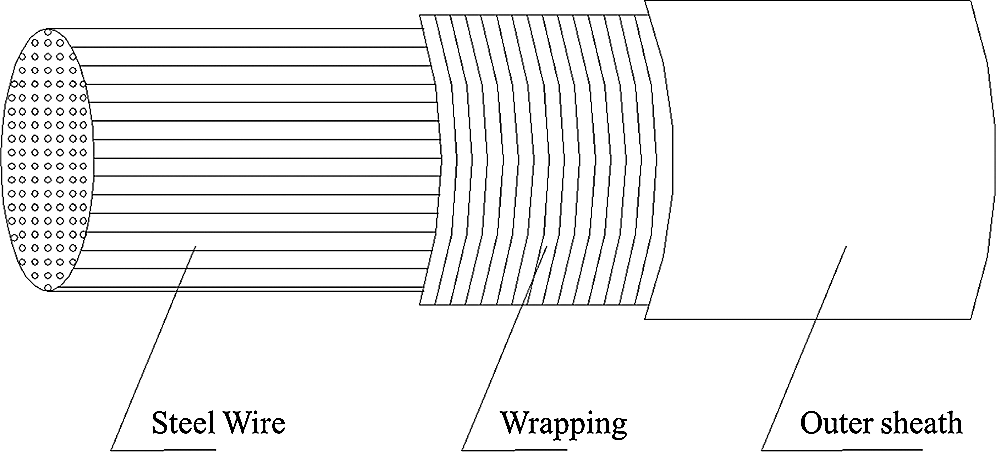
Figure 1: Main cable structure

Many scholars have studied and optimized a main cable dehumidification system. Jensen et al. [6] analyzed the causes of water ingress into different main cable systems, and the advantages and disadvantages of different main cable mitigation measures. The main cable dehumidification technology was introduced in detail, and the possibility of applying dehumidification technology in cable-stayed bridges was discussed. Kitagawa et al. [7] developed a dry air injection system for reducing corrosion in a suspension bridge. He also studied a new method for examining corrosion. Waldvogel et al. [8] introduced the first application of a main cable dehumidification system in North America and discussed controlling the system quality during field construction, based on, e.g., cable wrapping trials and field air flow trials. Bloomstine [9] presented a general description of corrosion protection using dehumidification, including full-scale and on-site testing. In addition, some scholars have made progress in regards to main cable material waterproofing, to protect from vapor corrosion. Wang et al. [10] proposed a method for improving a main cable material with basalt fiber-reinforced polymer (FRP). The combination of basalt and carbon fibers increased the fatigue performance and corrosion resistance of the main cable. Yang et al. [11] conducted a life cycle cost analysis on different main cable materials. The results showed that the life cycle cost of suspension bridges with FRP cables is higher than that of traditional steel cables, owing to the higher corrosion resistance and fatigue resistance of the FRP cables.

However, there has been no research on the flow resistance of dry air in the main cable. A main cable is made of thousands of steel wires. Air flows through the gaps of the wires, leading to an irregular cross-section. The bending wire also leads to gap bending. Both the irregular cross-section and bending wires make the calculation unique and difficult. In this study, based on a porous medium model and capillary bundle model, the flow resistance in the main cable is analyzed in depth, and a formula is obtained for the bending coefficient. Through experimental research to determine the bending coefficient, a semi-an empirical formula is obtained for the flow resistance. The accuracy of the semi-empirical formula proposed in this study is verified by simulation modeling and field measurements of a main cable.

2  Mathematical Proof and Calculation

The main cable of a suspension bridge is an accumulated porous medium, and the air flow in the main cable can thus be considered as the air flow in a porous medium, as found in nature. Models for studying the flow resistance in a porous medium include the average hydraulic radius model, capillary model, gap model, flow resistance model, and statistical model [12–16]. The average hydraulic radius model considers the flow in the porous medium as a flow with an uneven cross-section and interpenetration, whereas the capillary model considers the flow in the porous medium as a flow in an even parallel cylindrical capillary tube.

2.1 Average Hydraulic Radius Model

Air flows into the main cable from the intake hood and flows out through the exhaust hood, as shown in Fig. 2. The air flowing in the main cable does not have a circular cross-section but flows through between the interspaces of the steel wires; thus, the cross-section must be irregular, as shown in Fig. 3. Owing to the curves of the steel wires, the air flows in the main cable are also irregular, i.e., quite different from the ordinary air flow in an ordinary pipeline.

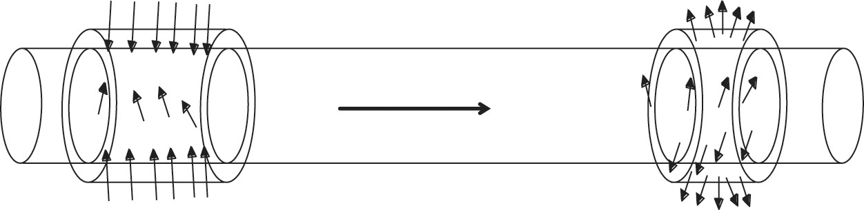
Figure 2: Air flow in the main cable

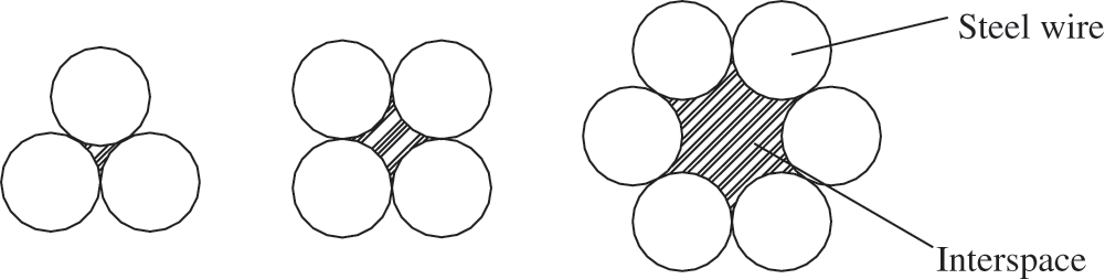
Figure 3: Interspace in the main cable

The study of the air flow process when adopting the average hydraulic radius model considers the circulation channel in the main cable as a circular tube of equivalent diameter. The pressure drop of the fluid flow in the main cable passage can be computed using the Hagen–Poiseuille formula [17] and the Darcy formula [18].

{Δpl=32μvd2d=4Ax=4Rh (1)

Here, Δp is the pressure drop (in Pa); l is the length (m); μ is the kinematic viscosity of air (kg/(s·m)); v is the fluid speed (m/s); d is the equivalent diameter (m); A is the circulation area (m2); x is the wetted perimeter (m); and Rh is the hydraulic radius (m).

Rh=Ax=VA1=V/VtA1/Vt=εa (2)

Here, V is the air circulation volume (m3), Vt is the main cable volume (m3), and A1 is the total wetting area (m2).

Each steel wire is considered to be composed of many smaller cylindrical steel wires, with a height equal to its diameter. The contact surface area of the air flowing in the main cable is the lateral area of the cylinder steel wire, and the specific surface of a cylindrical steel wire with a height equal to the diameter is the ratio between the lateral area and volume of the steel wire (the lateral area is two-thirds of the surface area of the cylindrical steel wire). If the ratio between the surface area and volume of the cylinder with the height equal to its diameter is aP , then the ratio between the contact area of the air with the cylinder steel wire and volume of the steel wire azl should be as follows:

azl=23ap (3)

Thus, the relationship between a and the specific surface of a section of the cylindrical steel wire azl is as follows:

a=azl(1−ε)=23ap(1−ε) (4)

In this relationship, ε is the porosity of the main cable [19]; a is the wetting area of a unit volume of the main cable (m2/m3); azl is the ratio of the contact area between the air and any one section of the cylindrical steel wire and its volume (m2/m3); and ap is the ratio between the surface area and volume of a cylinder with a height equal to its diameter (m2/m3).

Two parameters are required to determine the character of a non-spherical particle, namely, the degree of sphericity and the equivalent diameter. The sphericity degree is also called the form factor. It expresses the difference between the particle form and a sphere, and is defined as the surface area of a sphere with the same volume as the particle divided by the surface area of the particle, as follows:

φS=S/SP (5)

Here, φS is the sphericity degree of the particle (or form factor), and is non-dimensional; S is the surface area of a sphere with the same volume as the particle (m2); and SP is the surface area of the particle (m2).

In engineering, a non-spherical particle is commonly replaced with a “equivalent” spherical particle to make some character of the non-spherical particle equivalent to that of the spherical particle. The diameter of such a spherical particle is called the equivalent diameter, and represents the size of the non-spherical particle. According to the equivalence theory, the equivalent diameter of a flow pass can be determined by adopting an isopycnic or equal specific surface area method.

The equivalent diameter of a non-spherical particle can be expressed by adopting the diameter of a spherical particle with the same volume as that of the particle, as follows:

de=6πVP3 (6)

Here, de is the isopycnic equivalent diameter of the particle (m); and VP is the volume of the particle (m3).

The specific surface area equivalent diameter of the non-spherical particle da can be expressed by adopting the diameter of a spherical particle with the same specific surface area, as follows:

da=6/aP (7)

Using Eqs. (6) and (7), the relationship between the isopycnic equivalent diameter and specific surface area equivalent diameter of the particle can be obtained as follows:

da=deφS (8)

The geometric proportion surface area equivalent diameter of a non-spherical particle must be smaller than the isopycnic equivalent diameter. The character of a non-spherical particle can be expressed by the above form factor and equivalent diameter, as follows:

{VP=π6de3SP=πde2φSap=6φSde (9)

Substituting Eqs. (9) into (4), a calculation is obtained as follows:

a=23ap(1−ε)=4da(1−ε)=4deφS(1−ε) (10)

The relationship between the apparent velocity of the main cable vs and average velocity of the main cable void v is as follows:

vs=v⋅ε (11)

According to Eqs. (1), (10), and (11), we can determine a relationship as follows:

Δpl=32μvd2=32μva216ε2=2μva2ε2=32μv(1−ε)2ε2(deφS)2=32μvs(1−ε)2ε3(deφS)2 (12)

The flow of air in the main cable void is a curve; therefore, we should consider the impact of the bendability on the flow resistance. Thus, the pressure drop when the fluid passes through a unit length of the main cable should be determined as follows:

Δpl=32μvτ(1−ε)2ε2(deφS)2=32μvsτ(1−ε)2ε3(deφS)2 (13)

In the formula, τ is the bending coefficient. According to the definition of the form factor, the height of the cylinder is equal to its diameter. Thus, we can compute the form factor of the cylinder as φS=0.874 .

2.2 Capillary Bundle Model

According to Eq. (1), we obtain a calculation as follows:

Δpl=32μvd2=32μv(4Rh)2=32μv(4×εd4(1−ε))2=32μv(1−ε)2ε2d2 (14)

Here, ap is the ratio between the surface area and volume of a cylinder with a height equal to its diameter; therefore, we can determine a further calculation as follows:

ap=2π(d2)2+πd⋅dπ(d2)2⋅d=6d (15)

According to Eqs. (7) and (8), we obtain a relationship as follows:

da=deφS=6ap=d (16)

Hence,

d=deφS (17)

Substituting Eqs. (17) into (12), we obtain an equation as follows:

Δpl=32μv(1−ε)2ε2d2=32μv(1−ε)2ε2(deφs)2=32μvs(1−ε)2ε3(deφS)2 (18)

Eq. (12) is the same as Eq. (18). This proves that the air flow in the main cable is equivalent to the flow of air in the porous medium of the spherical particle. According to Eq. (13), only τ is unknown; thus, we should perform an experiment to calculate it.

2.3 Applicable Condition

Eq. (18) is only applicable to the laminar region, and the modified Reynolds number should satisfy certain conditions as follows:

{deG0μ(1−ε)<10G0=ρvs=ρvε (19)

Here, de is the diameter of the equivalent spherical particle (m); G0 is the mass flow through a unit area (kg/m2·s); μ is the kinetic viscosity coefficient of the flow (Pa·s); ε is the porosity; ρ is the air density (kg/m3); vs is the representation velocity (m/s); and v is the air velocity in the main cable (m/s).

The diameter of the main cable steel wire was 5.2 mm. The porosity of the cable was 0.2. The main cable was 6 m long, and the diameter of the main cable was 432.8 mm. We can solve for the applicable flow velocity range in Eqs. (18) using (19).

Using Eq. (6), we can compute the equivalent diameter of the main cable steel wire as follows:

de=6πVP3=6π×π(d2)2×d3=643d=1.145d=1.145×5.2=5.954mm (20)

According to Eq. (19), we obtain deρvεμ(1−ε)<10 . After substituting the specific data into it, we obtain v<0.1m/mss . A flow velocity of 0.1 m/s is much larger than the flow velocity in a main cable in actual engineering [20]; thus, Eq. (18) can be applied in actual engineering.

3  Experimental Study

To obtain the flow resistance in the main cable, a laboratory table was set up, as shown in Fig. 4. Photographs of the setup are shown in Fig. 5. The test procedure was as follows. First, dismantle the end cover shown in Fig. 4, and close the inlet air tube 11 and piezometer tube 5; then, air enters the plenum chamber 9, flows in from the right side of the main cable, and flows out from the left side. Piezometer tube 10 sends a pressure signal to a manometer, and adjusts the air supply flow according to the working conditions listed in Tab. 2 to ensure that the flow meets the requirements of each working condition. The pressure data is read when stable, to obtain the flow resistance under different working conditions.

Figure 4: Experimental model. 1-end cover 2-rubbergasket 3-cylinder of inlet chamber 4-front shroud of inlet chamber 5-piezometer tube 6-exhaust pipe 7-back shroud of inlet chamber 8-back end cover 9-plenum chamber 10-piezometer tube 11-inlet air tube 12-main cable model 13-wire wrapping 14-cover layer 15-tie rod 16-inlet air tube

Figure 5: Experimental photos

The main purpose of the experiment was to obtain flow resistance data that can be regressed to determine the bending coefficient τ in Eq. (13). To simulate an actual main cable, the experiment used one piece of main cable; thus, the working condition of the experiment approximated an actual working condition. The diameter of the steel wire was 5.2 mm, i.e., the same as that of an actual main cable (see Tab. 1 for specific parameters).

The porosity of the main cable must meet the requirements of actual engineering, i.e., no greater than 20%, and the laboratory table should have good sealing. Moreover, after erecting the laboratory table, the main cable model should be inclined toward different angles, to meet the requirements for simulating different working conditions.

To determine the air parameters in the main cable, pressure sensors were embedded at 30 testing points in the main cable model. One testing point was set in the intake hood on the left side, and the other was positioned in the plenum chamber on the right side. Seven testing points were set in each of the Sections 1-1, 2-2, 3-3, and 4-4 in the model. The positions of the sensors in each section are shown in Fig. 6. For each section, the smaller four measuring points measured the air velocity, and the larger three points measured the pressure. The positions of the sensors in the main cable model are shown in Fig. 7. When the air flowed from Section 1-1 to the left-side section of the main cable model, the measured data were analyzed in four sections, to obtain the flow resistance of the main cable model.

Figure 6: Sensor positions in section model

Figure 7: Sensor location schematic for the main cable

A McMillan Model 50 flowmeter was used to obtain the flow measurements, and the pressure measurements were made using a DST6800-DR micro-differential pressure gauge. The characteristics of the testing devices are listed in Tab. 3. To ensure the measurement accuracy, for every measured section, each parameter χ was measured three times to verify that the measurements met their requirements; otherwise, they were repeated.

maxχ−minχmaxχ≤0.05 (21)

As the gas flowed from the right side to the left side, the flow resistance loss was invariable. Under the same flow velocity, the unit length loss of the flow resistance was the same, and the pressure drop curve should be a straight line. For the main cable model, during the airflow process, the unit length flow resistance was determined as follows:

h′=pm−pnlm−ln (22)

Here, h′ is the flow resistance of a unit length, pm is the pressure in section m, pn is the pressure of section n, and lm−ln is the distance between two sections. The computed flow resistances of the main cables in the models are shown in Fig. 8.

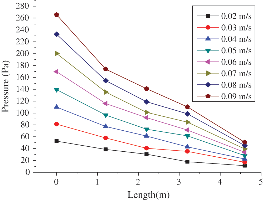
Figure 8: Pressure distribution in model

Fig. 9 shows the unit flow resistance of the main cable under various flow velocities.

Figure 9: Relation between air flow velocity and resistance in the main cable model

After fitting the experimental data using the least squares method, a computational formula for the unit length flow resistance pressure drop of the air flow in the main cable was obtained, as follows:

ΔpmL=0.02917+397.08333v. (23)

Here, Δpm/ΔpmLL is the pressure drop per unit length in the main cable model (Pa/m), and v is the air flow velocity in the main cable (m/s).

When the air flow velocity in the main cable is equal, the computational results of Eqs. (22) and (13) should be equal, and a bending coefficient τ=1.16 is obtained. Substituting φS=0.874 and τ=1.16 into Eq. (13) gives Eq. (23), i.e., a semi-empirical formula of the air flow resistance in the main cable.

Δpl=48.59μv(1−ε)2ε2de2=48.59μvs(1−ε)2ε3de2. (24)

4  Numerical Simulation

Fluent software was used for a simulation of air flow resistance. The simulation model was the same as the experimental model. The simulation adopted a porous medium model in Fluent to simulate the air flow in the main cable; the porosity was 19.8%, and the air flow velocity ranged from 0.02 m/s to 0.09 m/s (see Fig. 10).

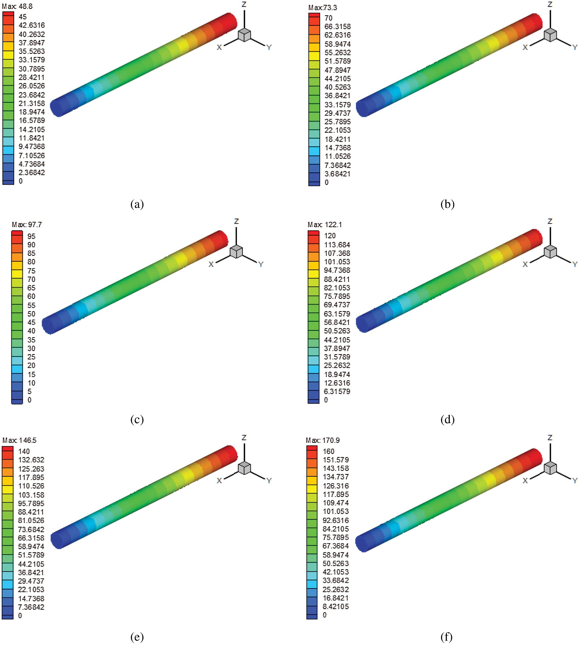
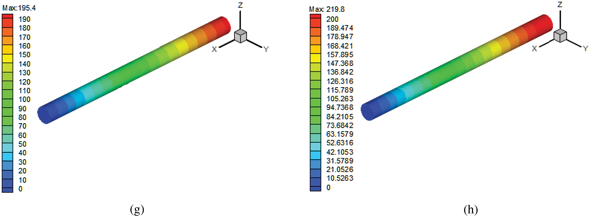
Figure 10: Pressure distribution for different air speeds of the main cable model. (a) v = 0.02 m/s, (b) v = 0.03 m/s, (c) v = 0.04 m/s, (d) v = 0.05 m/s, (e) v = 0.06 m/s, (f) v = 0.07 m/s, (g) v = 0.08 m/s and (h) v = 0.09 m/s

The simulation model was divided into six steps, as described below:

1. The length of the main cable model was set as 6 m, the diameter as 432.8 mm, and the porosity as 19.8%. In the Fluent software, the coordinates were Xmin = 100 mm, Xmax = 6100 mm, Ymin = −216.4 mm, Ymax = 216.4 mm, Zmin = −216.4 mm, and Zmax = 216.4 mm. The resistance numerical simulation of the main cable model was conducted with air velocities of 0.2, 0.3, 0.4, 0.5, 0.6, 0.7, 0.8, and 0.9 m/s. The grid spacing was 0.04 m, the main cable model node number was 33968, and the grid number was 158837.

2. The non-coupled implicit solver was selected for the steady-state conditions to solve for the flow field, and the physical velocity in the porous formulation area of the solver panel was selected for calculation. The laminar calculation model was also selected.

3. The desired fluid name was selected in the Material Name. The editing function was used (if necessary) to change the fluid parameter settings.

4. The inlet, outlet, and solid boundary conditions were set, the velocity inlet boundary condition and pressure outlet boundary condition were selected, and the fluid area was set as a porous area.

5. The monitoring volume and number of iterations were set, the calculation model was initialized, and the file was saved.

6. Iterative calculations were conducted, and Tecplot software was used to post-process the calculation results.

The simulation results are shown in Fig. 11. As the speed increased, the resistance of the air flow in the main cable increased accordingly.

Figure 11: Comparison of experimental and simulated values

As shown in Fig. 11, Fluent software can be used to simulate the trend of an air pressure drop in the main cable; the deviation between the simulated and experimental values is always less than 3%. The method of calculating the pressure drop using the computational model in Fluent software can meet the requirements for engineering calculations. Compared with other solution models, the solution model in this study has the following characteristics.

The simplified model for the porous media does not need to draw all the main cable wires in the gambit, and the parameter settings for the simplified model of porous media can be determined according to the research situation. Some qualitative parameters can be calculated and determined based on experimental data, such as the viscosity resistance coefficient. Using the simplified model in the Fluent software to calculate the air flow resistance in the main cable can lead to an improved prediction of the change law of the air flow pressure drop in a main cable with the air velocity at low flow rates.

The simplified model can only describe the change in the air flow velocity in the main cable approximately, and cannot reflect the actual change. In the simulation process, the simulated air flow is not identical to the actual flow process. Thus, the simulation results need to be compared with the test results, and a small gap should be allowed.

5  Bridge Verification

The Yangtze River Bridge comprises three towers and two spans, and its span is divided into sections of 390 m + 1080 m + 1080 m + 390 m. There are two main cables in the bridge, each with an average length of 3109 m. The cables are made of hot-dip galvanized high-strength steel wire with a diameter of 5.0–5.5 mm, constructed using air spinning or prefabricated parallel wire strands. Each main cable contains 184 parallel steel wire cables. Each wire cable has an average length of 2580.8 m and contains 127 hot-dip galvanized high-strength steel wires with diameters of 5.3 mm; each main cable contains 23268 wires in total. Each main cable weighs 1,0583.6 tons, and the internal void ratio of the main cable is approximately 20%. These steel wires are wound with wrapping and an outer sheath. To verify the accuracy of the semi-empirical formula and simulation, a field test was performed on the Yangtze River Bridge. The results were compared to flow resistance test data calculated using the semi-empirical formula.

To ensure the accuracy of the experiment, two sets of experiments were conducted, and the measurement regions were the same length (AB) and (CD). AC is the air inlet, and BD is the exhaust; AB and CD were both 18 m long. Pressure sensors were set at Points A, B, C, and D, and the pressure values were recorded. Field photographs are shown in Fig. 12.

Figure 12: Field experiment

The length of the main cable in the experiment was 18 m, and the diameter was 906 mm. The main cable included 184 strands of parallel steel wires, each containing 127 parallel steel wires (each with a diameter of 5.3 mm). The total volume of the air supply was Q, the sectional area of the main cable was S = 6447 cm2, and the porosity was 0.2. Based on the testing time, the average velocity of the air flow in the main cable was calculated.

v=QST=Q6447×10−4×0.2T=7.76QT (25)

Experiment 1: The experimental results obtained when the Roots blower frequency converter was adjusted to 54.6 Hz are shown in Tab. 4.

Experiment 2: The experimental results obtained when the Roots blower frequency converter was adjusted to 38.2 Hz are shown in Tab. 5.

The average airflow velocity ν in the main cable of Experiment 1 was as follows:

ν=7.76QT=7.76×0.9350=0.0199m/s (26)

Using formula (23), the resistance pressure drop of the experimental section was obtained through computation, as follows:

Δp=48.59μv(1−ε)2lε2de2=130.61Pa. (27)

The average air flow velocity ν in the main cable in Experiment 2 was as follows:

ν=7.76QT=7.76×0.9221=0.0317m/s (28)

Using Eq. (23), the resistance pressure drop of the experimental section was calculated as follows:

Δp=48.59μv(1−ε)2lε2de2=206.71Pa. (29)

The numerical simulation results for the flow resistance in the main cable of the bridge are shown in Fig. 13. When the flow velocity was 0.0199 m/s, the flow resistance pressure drop in the experimental section of the main cable was 131.7 Pa, and when the flow velocity was 0.0317 m/s, the flow resistance pressure drop was 208.4 Pa.

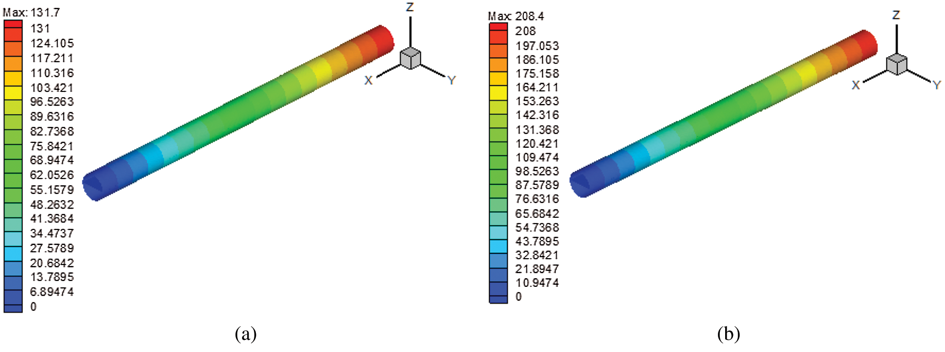
Figure 13: Numerical simulation results of the main cable flow resistance of the bridge. (a) Air flow velocity was 0.0199 m/s and (b) Air flow velocity was 0.0317 m/s

The calculated values (according to the semi-empirical formula) and numerical simulation results for the main cable flow resistance in Experiments 1 and 2 are shown in Tab. 6.

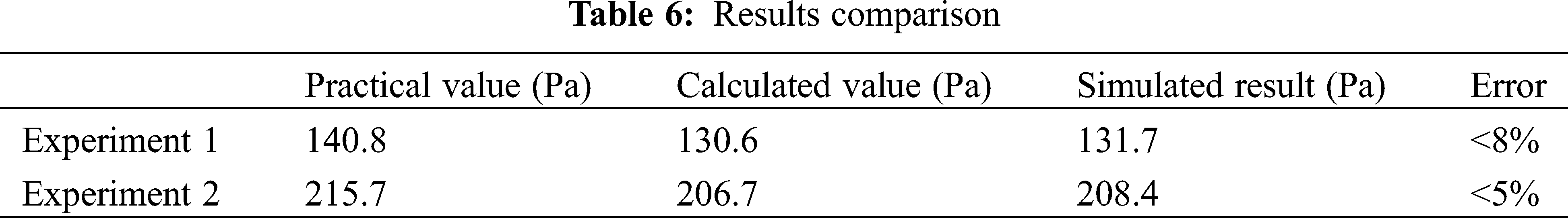
The results in Tab. 6 indicate that the calculated values and numerical simulation results from the semi-empirical formula are basically identical to the measured values. The largest error was only 8%; therefore, the semi-empirical formula can be utilized to solve for the air flow resistance in a main cable.

6  Conclusion

1.    Based on a porous medium model and capillary bundle model, the Hagen-Poiseuille formula is adopted. An average hydraulic radius resistance model is used to perform a mathematical derivation of the air flow resistance in the main cable, to thereby obtain an identical formula. This indicates that the equivalence of the air flow in the main cable to that in a porous medium is correct. The air flow in the void of the main cable follows a curve; therefore, we should consider the impact of the bendability on the flow resistance. The bending coefficient τ can be determined experimentally.

2.    The study determines the air flow resistance value in the main cable using an empirical model. It solves for the bending coefficient in the air flow resistance computational formula of the main cable to obtain a semi-empirical formula for the flow resistance in the main cable.

3.    Using Fluent, the air flow resistance in the main cable is computed, along with the change law of the air flow pressure drop with changes in the air flow velocity in the main cable.

4.    To verify the correctness of the semi-empirical formula, a field test was conducted on the air flow resistance in the Yangtze River bridge. The measured resistance value was basically identical to that calculated through the semi-empirical formula, providing validation for the formula.

The air flow resistance in the main cable has a very important influence on the drying of the main cable. Based on the semi-empirical formula determined in this study, a designer can choose an appropriate air supply fan pressure and air volume under different main cable parameters. Furthermore, it is possible to determine the annual operating energy consumption of the main cable dehumidification system, which has significant practical significance in energy saving control.

Acknowledgement: We gratefully acknowledge the kind assistance of Dr. Luyan Sui and Dr. Guanzhong Peng in the preparation of this article.

Funding Statement: Ministry of Communications and Provincial and Joint Research Project [2008-353-332-170].

Conflicts of Interest: The authors declare that there is no conflict of interest regarding the publication of this paper.

This work is licensed under a Creative Commons Attribution 4.0 International License, which permits unrestricted use, distribution, and reproduction in any medium, provided the original work is properly cited.