Fluid Dynamics & Materials Processing

DOI: 10.32604/fdmp.2021.014470

ARTICLE

A New Processing Method for the Nonlinear Signals Produced by Electromagnetic Flowmeters in Conditions of Pipe Partial Filling

Yulin Jiang*

College of Information Engineering, Zhongshan Polytechnic College, Zhongshan, 528404, China
*Corresponding Author: Yulin Jiang. Email: ghostjiang@sina.com
Received: 29 September 2020; Accepted: 24 February 2021

1  Introduction

Electromagnetic flowmeters are widely used for various types of measurements due to the advantages of high measurement accuracy and wide measurement range. The measurement principle of the electromagnetic flowmeter bases on Faraday’s law of electromagnetic induction. When the measuring pipe is completely filled, the average flow velocity of the fluid is linearly proportional to the induced electromotive force (EMF) of the electrode sensor [1–6], and the flow rate of the fluid can be measured by the induced EMF of the sensor. However, when the pipeline is only partially filled, the relationship between the average velocity and the sensor-induced EMF is nonlinear [7–11]. The relationship varies with different parameters, such as the pipeline filling, pipe wall friction coefficient, and fluid density. In the field of flow measurement, nonlinear data are converted into estimated linear data, and data compensation is performed to reduce the error. For different pipe diameters, pipe friction coefficients, installation methods, measurement fluids, and other parameters, different compensation values are expected. However, in the measurement, the measured data is compensated based on the experimental data. If parameters such as the sensor geometry and the friction coefficient of the pipe wall change, the accuracy of real time measurements decreases significantly. Therefore, it is important to find a nonlinear signal processing method that is suitable for data processing of a partially filled electromagnetic flowmeter.

In the field of nonlinear signal processing, a series of studies with many significant research results have been reported [12–18]. Hudson et al. [12] applied nonlinear signal processing techniques to neural networks to extract simple dynamic models from complex experimental time series. Dinis et al. [13] combined nonlinear signal processing with frequency filtering to process multiple digital signals of orthogonal frequency division multiplexing (OFDM), which reduced the envelope fluctuation of ordinary OFDM while keeping its high spectral efficiency to achieve a low-cost, power-efficient implementation. Mokhtari [15] proposed a nonlinear adaptive cooperative controller, which can develop an SAC-like adaptive SC law by modifying the original SC law, as has been verified on four rotor aircraft. Jahmunah et al. [16] used a nonlinear processing method to automatically monitor and evaluate patients with schizophrenia. Nonlinear signal processing methods have been extensively used in various fields of life. However, most of these methods use offline data processing with the computer microprocessor. Partially filled electromagnetic flowmeters have two major challenges in offline data processing, which are difficult to resolve. First, because the electromagnetic flowmeter needs to display the fluid flow rate, flow velocity, and other features in real time, it is not suitable for offline data processing. Secondly, the price of an ordinary electromagnetic flowmeter is low, and the microprocessors used in the circuit usually have a low performance, which makes them not suitable for an online signal processing method for nonlinear signals. The application of nonlinear processing with low-performance microprocessors is limited in the field of flow measurement. Therefore, it is necessary to find a method that can convert nonlinear signal processing into a method suitable for low-performance microprocessors.

B-spline curve fitting [19–23] is an approach that performs a nonlinear fit of data based on a limited selection of these data. As the B-spline curve method is a simple calculation procedure with fast calculation speed and geometric invariance, it is widely used in engineering practice, such as for the geometric definition of various industrial products and nonlinear curve reconstruction. Gao et al. [20] proposed a double B-Spline curve fitting and synchronization-integrated federate scheduling method for a Five-Axis linear-segment tool path, and simulation showed that this method can generate a smooth tool path and constrain the fitting error. Xu et al. [21] rebuilt the strain field of multiple elements by using the B-spline curve and inverse finite element methods to prove that the proposed algorithm can significantly improve the accuracy of reconstruction displacement. Jiang et al. [22] reconstructed the under-sampling flow velocity distribution of partially filled pipes using the B-spline curve method, showing that this method effectively reduces the number of measurement data. Ravari et al. [23] improved the B-spline curve method by using the group test theory to effectively enhance the low data processing efficiency of the B-spline curve fitting method. Obviously, the B-spline curve fitting method was powerful in the processing of nonlinear data. The fitting accuracy of the B-spline curve method has been reported to be higher than that of the commonly used least squares method in the processing of nonlinear data [24–26]. However, dealing with nonlinear data by using the B-spline curve method, requires complex matrix inversion. Due to the limited microprocessor performance, the microprocessor of the electromagnetic flowmeter cannot complete the matrix inversion online, which greatly limits the application of the B-spline curve method in the online measurement of the electromagnetic flowmeter.

To solve the problems of the B-spline curve method in engineering applications, an improved B-spline curve fitting method is proposed, which can process the nonlinear signal of partially filled electromagnetic flowmeter online. First, based on the original definition of B-spline curve fitting, the control vertex sequence involved in matrix inversion was analyzed, and the general expression of control vertex was obtained. Second, the deviation between measured and fitting data was analyzed by the least square method, and the expression of the control vertex based on the minimum error was obtained. Finally, the control vertex expression was analyzed, and matrix inversion was converted into a mixed operation consisting of simple addition, subtraction, multiplication, and division by using the recursive method, so ordinary microprocessors can solve the B-spline curve method online. Our experimental results proved the feasibility of the proposed method.

This paper is divided into four parts: (1) The measurement principle and existing problems of partially filled electromagnetic flowmeters; (2) traditional B-spline curve method; (3) improvement of key features of the B-spline curve method; and (4) experimental design and verification.

2  The Measurement Principle and Existing Problems

In this section, the measurement principle of the traditional electromagnetic flowmeter is introduced, and existing problems in the online measurement of partially filled pipelines is analyzed.

2.1 Measuring Principle of the Point Electrode Electromagnetic Flowmeter

The schematic diagram of the traditional point electrode electromagnetic flowmeter [4] is shown in Fig. 1.

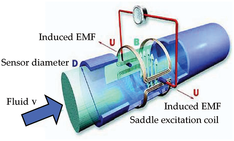
Figure 1: Schematic diagram of an electromagnetic flowmeter

According to Faraday’s law of electromagnetic induction, an electromotive force proportional to the average velocity will be generated between the two electrodes when a fluid flows through the applied magnetic field of the electromagnetic flowmeter. The direction of the electromotive force is perpendicular to the electrodes and parallel to the fluid flow and the magnetic field. The induced electromotive force difference E of the sensor can be expressed by the following formula [1–4]:

E=1πRL∫Z=−LL∫θ=02π∫r=0RBνWrdrdθdz (1)

where E is the induced electromotive force difference between the two sensor electrodes, L is half of the length of the electromagnetic flowmeter, B is the magnetic induction intensity of the electromagnetic flowmeter, R is the hydraulic radius of the measuring pipeline, v is the flow velocity of the fluid, and W is the body weight function, which is used to express the contribution of each part of the fluid to the EMF induced between the electrodes. The size of the weight function can be obtained by solving the basic differential equation of the electromagnetic flowmeter [1,27]. When the pipeline is completely filled with fluid, the geometric boundary conditions of the electromagnetic flowmeter remain unchanged. Under the premise that the value of the weight function W=1 , the flow velocity and magnetic field strength at each point are equal, and the difference of the induced EMF of the electrodes can be expressed by the following formula [1,6]:

E=BDν¯ (2)

where ν¯ is the average velocity of the measured fluid, and D is the hydraulic diameter of the pipe. This equation indicates that, the relationship between the induced EMF difference of the sensor and the average velocity of the fluid is monotonic and linear for W = 1. Therefore, the average flow velocity of the electromagnetic flowmeter can be directly calculated by the sensor-induced EMF when the pipe is completely filled.

2.2 Problems in the Online Measurement

However, in engineering applications, pipelines are often only partially filled with fluid, and the boundary conditions of the sensor vary with the change of the fluid level of the pipeline. The relationship between the induced EMF difference of the sensor and the average velocity of the fluid is non-monotonic and nonlinear. Computing the average velocity or flow rate according to the relationship shown in formula (2) inevitably causes larger errors, which are usually reduced experimentally. When the electromagnetic flowmeter was manufactured, a large number of experiments were carried out to measure parameters such as the induced EMF, flow velocity, and flow rate at different fluid levels. The relationship between the induced EMF and the flow rate was approximated by linear interpolation. However, when the installation of the measuring pipeline is inclined, the density of the conductive fluid, the friction of the pipeline, the sensitivity of the sensor electrode, and other factors change, resulting in deviations between real time measured data and predicted data at the time of production, which presents a difficulty that needs to be overcome. Therefore, it is inadequate to replace the actual measurement data with experimental data. Nevertheless, for the traditional point electrode electromagnetic flowmeter, when pipeline is partially filled with fluid, only a very limited amount of data can be collected, which cannot meet the requirements of CPU programming. Therefore, the focus of this paper is the use of limited measurement data for the online prediction of the overall data.

The B-spline curve fitting method can reconstruct the whole data based on a limited number of measurement data. As the B-spline curve method has the characteristics of geometric invariance, convex hull, and local support, the B-spline curve reconstruction method based on measurement data is one of the key technologies of reverse engineering. In the process of calculation, only three measurement data are needed to complete the reconstruction of the curve, and increasing the number of measurement data can improve the accuracy of the reconstruction. Therefore, this paper uses the B-spline curve method to solve the problem of inadequate measurement data in the online measurement of the partially filled electromagnetic flowmeter.

3  Key Parameters of the B-Spline Curve Method

This section mainly introduces the basic principle of the B-spline curve method, combined with the sample data of the electromagnetic flowmeter, and the expression of the control vertex was obtained using the least square method.

3.1 Traditional B-Spline Curve Method

When the induced EMF output by the electromagnetic flowmeter sensor is Ej(j=1,2,⋯,n) and the corresponding fluid flow rate is qj(j=1,2,⋯,n) , q=f(E) can be described by the following B-spline curve fitting equation [21–23]

q=∑i=0Nmi,k(E)piE∈[uk−1,uN+1] (3)

where k is the order of the B-spline curve, N is the number of nodes obtained by internal division of the vector Ej(j=1,2,⋯,n) , pi(i=1,2,⋯,N) is the control vertex column vector, and mi,k(E) is the basis function of the k -order B-spline curve.

According to the internal node sequence Ei(i=1,2,3,⋯,N) of the re-divided measurement data and basis function mi,k(E) , the control vertex pi of the B-spline fitting curve can be expressed as [19]

Pn=(MnTMn)−1E (4)

where T represents the matrix transposition operation, the exponent “–1” indicates matrix inversion, and E=[E0,E1,E2,⋯EN]T is the matrix representation of the measurement data sequence. By solving Eq. (4) with the Gaussian elimination method [28,29], the control vertex sequence Pn=[p0,p1,⋯,pN]T can be obtained. Mn is the matrix representation of the basis function, which can be expressed as follows:

Mn=[m1,0m1,1⋯m1,Nm2,0m2,1⋯m2,N⋮⋮⋮⋮mn,0mn,1⋯mn,N] (5)

Eq. (4) is a general expression of the control vertex, and a more explicit expression can be obtained by further solving the equation with the measured data. In this paper, the least squares method based on the minimum mean square error was used to further process the control vertex expression.

3.2 Control Vertex Expression Based on Least Square Method

By substituting the measured sample data dj={Ej,qj}j=1n into Eq. (3), the measured data can be approximated by the B-spline fitting curve according to

qj(E)=∑i=0Npimi,k(E)+sjj=1,2,3,⋯,n (6)

where sj is the deviation between the measured data and the fitted data. Eq. (6) can be expressed in matrix form as

Qn=PnMn+Sn (7)

where Qn=[q1,q2,q3,⋯,qn]T is the matrix representation of the flow signal, and Sn=[s1,s2,s3,⋯,sn]T is the matrix representation of the deviation. Then, the square of the deviation between the measured data and the fitted curve data can be expressed as

ε=[Qn−PnMn]T[Qn−PnMn] (8)

According to the computation principle of the least square method, when ∂ϵ/∂ϵ∂Pn∂Pn=0 , the value of ϵ is the smallest, and the control vertex Pn can be expressed as

Pn′=[MnTMn]−1MnTQn (9)

To solve the sequence of the control vertex sequence with the least square method, matrix inversion must be performed. Since the measurement results of the electromagnetic flowmeter need to be displayed in real time, all the data must be processed by a computer. However, the calculation of the inverse matrix is a significant challenge for commercial microprocessors of ordinary point electrode electromagnetic flowmeter. Therefore, in order to find a suitable solution method, formula (9) must be further analyzed and optimized.

4  Optimal Solution Method of Control Vertex

According to the previous analysis, the B-spline curve method involves the complex matrix inversion for the calculation of the control vertex. However, the microprocessor of the ordinary flowmeter cannot calculate the inverse of the matrix online, so the solution process must be further optimized. According to Eq. (9), the control vertex sequence is expressed a Pn′ for the smallest deviation between the measured data and the fitted curve, and the number of measurements is n. For n + 1 measurements, the control vertex sequence can be written as Pn+1′ . Referring to Eq. (9), Pn+1′ can be expressed as

Pn+1′=[Mn+1TMn+1]−1Mn+1TQn+1 (10)

For Fn+1=[mn+1,0,mn+1,1,⋯,mn+1,N] , , Mn+1TMn+1 in Eq. (10) can be expressed as

Mn+1TMn+1=[MnTFn+1T][MnFn+1] (11)

Substituting formula (11) into formula (10) resulted in

Pn+1′=[[MnTFn+1T][MnFn+1]]−1[MnTFn+1T][Qnqn+1]=[MnTMn+Fn+1TFn+1]−1[MnTQn+Fn+1Tqn+1] (12)

From Eqs. (9) and (12), the following relationship between pn+1′ and pn′ was derived:

Pn+1′−Pn′=[MnTMn+Fn+1TFn+1]−1[MnTQn+Fn+1Tqn+1]−[MnTMn]−1MnTQn=[MnTMn+Fn+1TFn+1]−1Fn+1T(qn+1−Fn+1Pn′) (13)

Then, the control vertex Pn+1′ can be expressed as

Pn+1′=Pn′+[MnTMn+Fn+1TFn+1]−1Fn+1T(qn+1−Fn+1Pn′)=Pn′+[Mn+1TMn+1]−1Fn+1T(qn+1−Fn+1Pn′) (14)

According to the matrix inversion lemma, [Mn+1TMn+1]−1 can also be expressed as

[Mn+1TMn+1]−1=[MnTMn]−1−[MnTMn]−1Fn+1T[1+Fn+1[MnTMn]−1Fn+1T]−1Fn+1[MnTMn]−1 (15)

with the initial value of the expression [Mn+1TMn+1]−1 of

[M0TM0]−1=c×IN+k (16)

where c is a sufficiently large real number, and I is the identity matrix. Then, the value of [MnTMn]−1 can be recursively obtained by Eqs. (15) and (16) without the need for matrix inversion.

Similarly, for an initial value of the control vertex of P0′=0 , Eq. (14) indicates that the control vertex Pn′ can be recursively obtained by Eq. (15) without the need for matrix inversion. Eqs. (14) and (15) were used to solve the control vertex sequence. As the solution does not involve matrix inversion, the requirements for the microprocessor performance are greatly reduced, which makes it possible to apply the B-spline curve fitting in the real-time online measurement.

5  Experimental Design and Verification

According to the basic laws of hydraulics, the mapping relationship between the sensor-induced EMF and the flow rate of different ordinary electromagnetic flowmeter are similar when the geometric structures of their measuring tubes are similar, such as the inclination of the pipeline, the friction coefficient of the tube wall, and other elements.

5.1 Experimental Device

A standard electromagnetic flowmeter was used to measure the flow of fluid in real time, and the experimental device is schematically depicted in Fig. 2. The diameter of this device was 32 mm, and the accuracy level was 0.3. The isolation plate in the water tank was utilized to ensure that the fluid is in a relatively stable state. The diameter of the test electromagnetic flowmeter was 50 mm, and the signal processing circuit was designed independently. The undeveloped state of the flow control valve was controlled to achieve different levels of the fluid flowing through the electromagnetic flowmeter. The electrode sensor was connected to the oscilloscope with a wire, and the induced EMF value of the electrode sensor was observed in real time for varying fluid levels of the pipe. A fluid level sensor was installed on the top of the measuring pipe to indicate whether the pipe is completely filled. When the pipeline is only partially filled with fluid, the fluid level of the fluid level sensor is high after passing through the circuit, while it is low when the pipeline is completely filled.

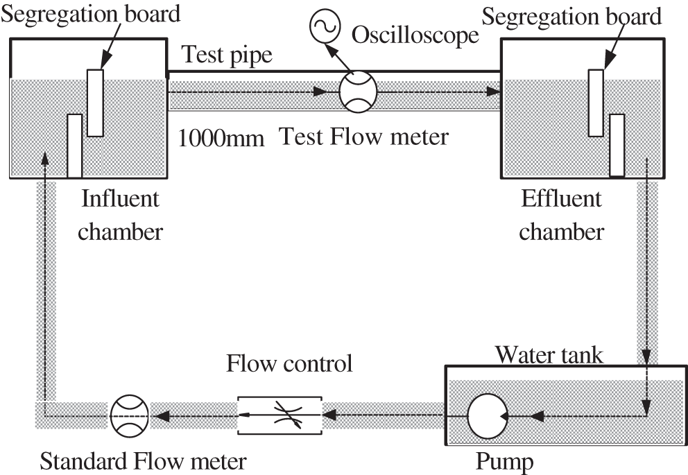
Figure 2: Schematic diagram of the experimental device

The test flowmeter was a general point electrode electromagnetic flowmeter, and the sensor electrodes were placed in the middle of the pipe wall. For a fluid level of less than 50%, the sensor produced no output value. However, in the actual measurement, an irregular fluctuating signal was obtained from the oscilloscope as the sensor signal of the empty pipe. At fluid levels higher than 50%, the output value of the sensor gradually stabilized. The induced signal output of the electrode sensor is a weak signal, which is easily interfered by various types of noise. The hardware circuit is used for signal amplification and noise filtering of the weak signal before the signal is transferred to the oscilloscope, and the amplification factor is 1000.

5.2 Experimental Results

After amplification, the induced EMF of the electrode sensor was read from the oscilloscope for different fluid levels. At the same time, the corresponding flow rate was read from the standard flowmeter. The measurement uncertainty of a measurement point can be expressed as

Su=∑i=1g(Ei−E¯)g(g−1) (17)

where g is the number of repeated measurements of a single measurement point, and E¯ is the average value of repeated measurements. The measurement uncertainties of all measurement points were calculated according to Eq. (17), showing that the uncertainty ranged from 0.00011 to 0.00096 and gradually increased from the middle of the pipe to the pipe wall. The measurement results are listed in Tab. 1.

Table 1: Measurement results for different fluid levels

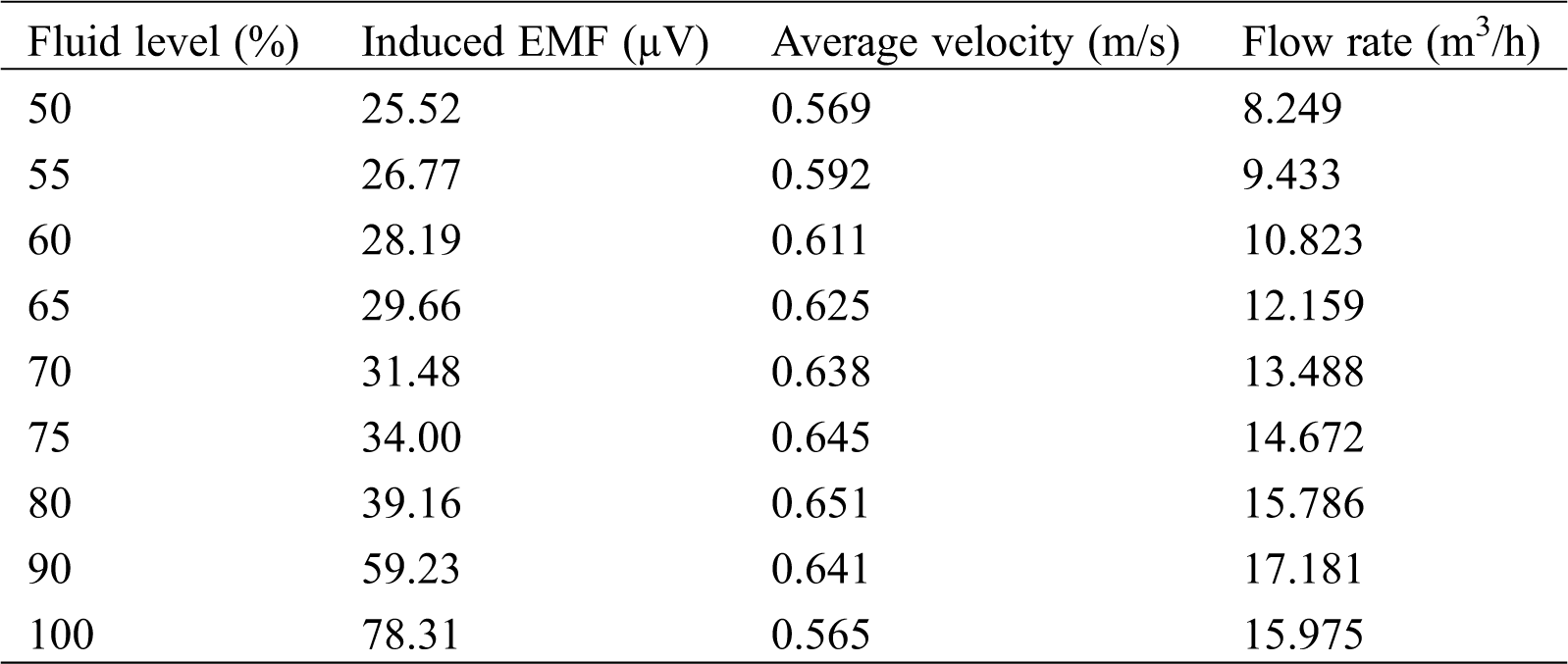
When the fluid level in the pipeline is higher than 80%, fluctuations in the fluid flow gradually increase in the process of measurement. The output signal of the sensor also fluctuates, and the uncertainty of the measurement exceeds 0.0005. Therefore, only results for a fluid level of 90% were considered, and the average value of multiple measurements was recorded. Tab. 1 lists the results for different fluid levels. According to these results, partially filled pipes revealed a nonlinear and non-monotonic relationship between the electrode-induced EMF and the average flow rate, as shown in Fig. 3. The induced EMF increased with the increase of the fluid level of the pipeline, as shown in Fig. 4. However, the average velocity of the fluid did not increase monotonously with the fluid level of the pipe. At a fluid level of about 80%, the velocity reached the maximum and then decreased (Fig. 5), which is consistent with the law of hydraulic motion of circular pipes. At the same time, the relationship between the output value of the electrode sensor and the flow rate is also nonlinear and non-monotonic. When the fluid level of the pipeline was 90%, the flow rate reached the maximum and then decreased, as shown in Fig. 6.

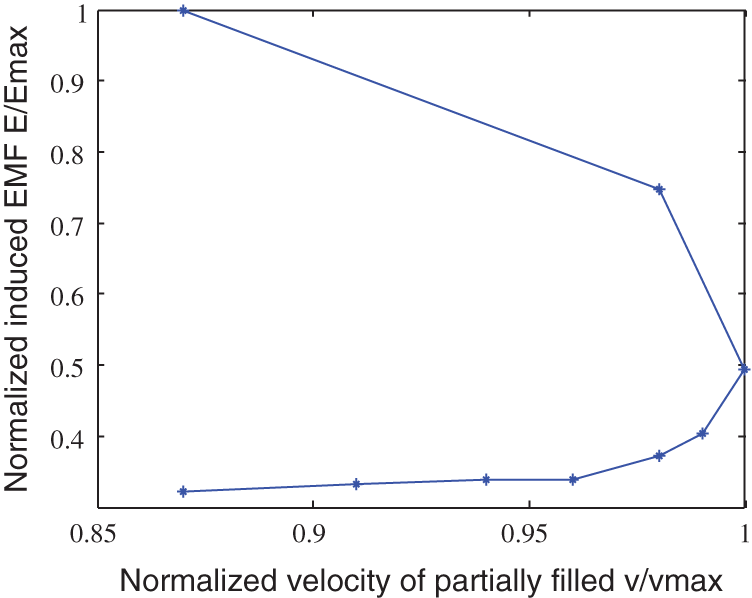
Figure 3: Average velocity-induced EMF characteristic curve (Emax, maximum induced EMF of the measurement sequence; vmax, maximum flow velocity)

Figure 4: Induced EMF characteristic curve at different fluid levels (Emax, maximum induced EMF of the measurement sequence)

Figure 5: Average flow velocity characteristic curve at different fluid levels (Vmax, maximum flow velocity)

Figure 6: Flow rate-induced electric potential characteristic curve (Emax, maximum induced EMF of the measurement sequence)

Fig. 3 reveals that the relationship between the induced EMF of the sensor and the average fluid velocity is non-monotonic and nonlinear, which is completely inconsistent with the relationship shown in Eq. (2). Therefore, the linear Eq. (2) cannot be used to process the nonlinear measurement data of the partially filled pipe.

The above data were obtained by using multiple instruments, such as oscilloscope and standard electromagnetic flowmeter. However, only one test electromagnetic flowmeter can be used in the real-time measurement, and the data for which the electromagnetic flowmeter can directly distinguish the corresponding position are limited. When the fluid level of the pipeline just reached 100%, the output value of the fluid level sensor dropped from a high to a low level. The relationship between the induced EMF of the sensor and the average flow rate follows Faraday’s law of electromagnetic induction. The microprocessor could easily determine the average velocity v100% and the flow rate q100%. When the fluid level in the pipeline just reached 50%, the induced EMF measured by the sensor tended to be stable, and the microprocessor easily captured the induced EMF of the electrode sensor. Figs. 3 and 6 showed that the average velocity v50% was similar to the average velocity v100% of the completely filled pipe, while the flow rate q50% was only 51.6% of the flow rate q100% of the completely filled pipe. According to the computational principle of the B-spline curve fitting method, at least three known measurement data are required to calculate the fitting parameters. If only two data points are available, the deviation between the fitting and measured data is large, so additional measurement data are needed.

5.3 Determination of New Feature Points

According to the basic laws of hydraulics, ordinary electromagnetic flowmeters have similar characteristic curves of induced EMF flow and induced EMF velocity when their geometrical structure, inclination, pipe wall friction, fluid density, and other parameters are similar. In this paper, the maximum curvature method proposed in literature [30,31] was used to add new feature points. The curvature was calculated according to following formula:

Kj=‖S′(dj)×S′′(dj)‖‖S′(dj)‖2j=0,1,⋯,n (18)

where dj={Ej,qj}j=1n is the measured sample data of the flow-induced EMF, the parametric polynomials S(d) were established based on the three points before and after the measured points, S′(dj) represents the first derivative of the curve at parameter dj , S′′(dj) represents the second derivative, and the magnitude of the curvature reflects the variation in the degree of flux. The curvature of the fluid level-flow rate characteristic curve is shown in Fig. 7.

Figure 7: Curvature of fluid level-flow characteristic curve

Fig. 7 shows the largest curvature of the fluid level-flow characteristic curve for a fluid level of 90%, and this point was selected as the feature point. For a fluid level of 90%, the output value of the electrode sensor was 75.6% of the completely filled pipe (Fig. 6). Similarly, the curvature distribution of the fluid level-average flow velocity characteristic curve was obtained according to formula (18), as shown in Fig. 8. The largest curvature was obtained for a fluid level of 80%, and this point was selected as the feature point of the fluid level-average velocity fitting curve. For a fluid level of 80%, the output value of the electrode sensor was about 50% of the completely filled pipe (Fig. 3).

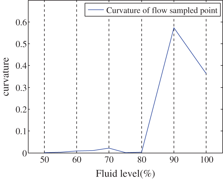
Figure 8: Curvature of fluid level-average velocity characteristic curve

5.4 Analysis of Experimental Results

The improved B-spline curve fitting method was used to predict the mapping relationship between the induced EMF and the flow rate. The data points {(E50%,q50%),(E80%,q90%),(E100%,q100%)} were taken as the sample data, and other measurement data were taken as the data for verification. In the experiment, the microprocessor model of the electromagnetic flowmeter was STM32F103C8T6. The proposed B-spline curve method was programmed on the Keil uVision5 MDK software platform to generate executable files and downloaded to the microprocessor to be run. According to the measurement sample data, the internal nodes were evenly divided at equal intervals. The number of internal nodes was 7. Appropriately increasing the number of internal nodes will increase the accuracy of fitting but also increase the amount of calculation. The value of each parameter was calculated by the parameterization method of the accumulated chord length, followed by the calculation of the node vector. The basis function of the B-spline curve was calculated according to the node vector, and the control vertex sequence was calculated using the method proposed in this paper. The coefficient C was set to an initial value of 10. Finally, the basis function and control vertex sequence were substituted into formula (3) to obtain the relationship between the fitting curve and the sensor-induced EMF, as shown in Fig. 9. The relative deviation between the measured sample data and the fitted data is given in Fig. 10. The maximum fitted relative deviation was 7.2%, and the formula of the relative deviation of the fitted curve was |sj|/qj×100%. Similarly, the data points {(E50%,v¯50%),(E80%,v¯80%),(E100%,v¯100%)} were taken as the sample data to obtain the average velocity fitting curve of the sensor-induced EMF, and the results are shown in Fig. 11. The relative deviation between the measured sample data and the fitted data is given in Fig. 12, revealing a maximum fitted relative deviation of 3.5%.

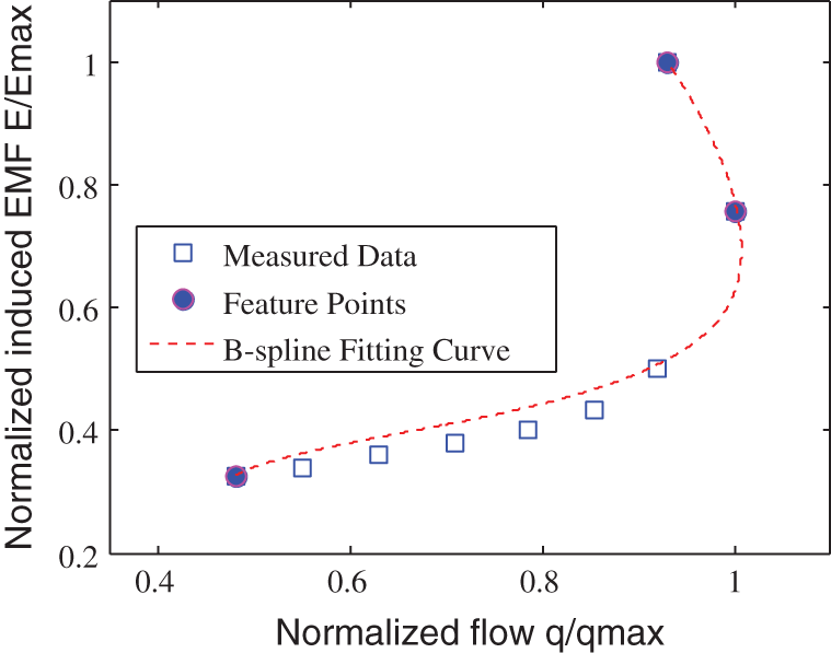
Figure 9: Normalized induced EMF-flow fitting curve

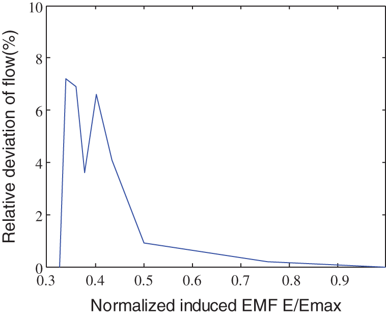
Figure 10: Induced EMF-flow fitting error

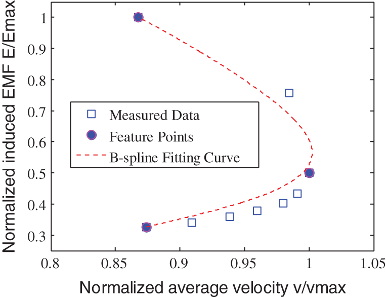
Figure 11: Normalized induced EMF-average velocity fitting curve

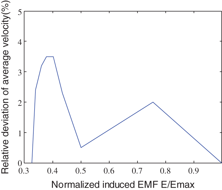
Figure 12: Induced EMF-average velocity fitting error

Figs. 9 to 12 show that the improved B-spline curve fitting method achieved a better prediction of the flow rate and the average velocity of the electromagnetic flowmeter in a partially filled state. The maximum relative deviation between the predicted average velocity and the measured data was 3.5%, which meets the requirements of typical industrial instruments, showing that the proposed improved B-spline curve fitting solving method is feasible. However, the maximum relative deviation between the predicted flow rate and the measured data was 7.2%, indicating that this method needs further improvement. To achieve more accurate predictions, different feature points need to be added. Matrix inversion is not required in the whole calculation process, which reduces the requirements for the performance of the microprocessor and is thus convenient for the real-time data processing with the microprocessor.

6  Conclusions

The difficulties of the ordinary point electrode electromagnetic flowmeter in the measurement of partially filled pipelines were analyzed in this paper. The B-spline curve method is suggested to solve lack of real-time data. The matrix inversion operation in the implementation process of the B-spline curve method is analyzed, and the matrix inverse operation was converted into a general mathematical operation, which reduces the performance requirements of the microprocessor. The method proposed in this paper obtains ideal real-time online measurement results with less sample data when the fluid level of the pipeline is greater than 50%. As all the sample data are real-time measurement data, the pipeline geometry, pipe wall friction coefficient, inclination, fluid density, and other working conditions are identical, resulting in an increased value of point electrode electromagnetic flowmeter for practical applications.

Funding Statement: This work was supported by the Science and Technology Project of Education Department of the Guangdong Province, China (2017GKTSCX079), and Science and Technology Project of Zhongshan Polytechnic, China (2018G01).

Conflicts of Interest: The author declares that they have no conflicts of interest to report regarding the present study.

This work is licensed under a Creative Commons Attribution 4.0 International License, which permits unrestricted use, distribution, and reproduction in any medium, provided the original work is properly cited.