Materials Processing
| Fluid Dynamics & Materials Processing |
DOI: 10.32604/fdmp.2021.015127
ARTICLE
Numerical Simulation of U-Shaped Metal Rings in a Wind-Sand Environment
College of Mechanical Engineering, Xinjiang University, Urumqi, 830000, China
*Corresponding Author: Xinmei Li. Email: lxmxj2009@126.com
Received: 24 November 2020; Accepted: 04 March 2021
Abstract: The interaction of U-shaped rings used for power transmission hardware with a wind-sand field is simulated numerically. A standard
Keywords: Wind-sand environment; connecting hardware; U-shaped ring; numerical simulation
More and more Ultra High Voltage (UHV) transmission lines have been built in recent years [1]. However, UHV transmission lines pass through region with the harsh environment, the annual average number of fresh gale is more than 100 days, and the maximum average wind velocity can reach 44 m/s [2,3]. Under strong wind environment, when the components such as power connection hardware (PCH) and wires are subjected to wind load, on the one hand, the flow characteristics around components will change. On the other hand, the PCH will be hit by sand grains, which not only cause erosion of the surface of the PCH, but also sand grains will enter the contact area of the hardware to accelerate the wear of hardware. This phenomenon not only cause lots of waste of human and financial resources, but also bring hidden dangers to the safe and reliable operation of transmission line. Therefore, it is necessary to study the aerodynamic performance of PCH in wind-sand field and clarify the characteristics of wind-sand around PCH.
Wear test on U-shaped ring of PCH under strong wind environment was studied to illustrate the failure mechanism by Yang [4]. Deng et al. [5] studied the wear of U-shaped rings in different wind-sand environments and concluded that the sand grains would accelerate the wear failure of hardware. The test was used to study the influence of wind, sand and other factors on the corona of transmission line hardware by Zhao et al. [6]. Using finite element software, Wang et al. [7] analyzed the static and dynamic characteristics of the U-shaped ring by numerical simulation and found that the U-shaped ring had the most serious deformation at the sixth order. Lu [8] used ANSYS to analyze the statics and dynamics of the U-shaped ring, and obtained the maximum equivalent stress and dangerous contact area of the U-shaped ring. The breeze vibrations were investigated on large transmission lines by Rawlins [9]. Urchegui et al. [10] studied the influence of different factors on the fretting wear of steel strand and put forward measures to alleviate the wear of steel strand. Lu [11] collected the climate information where the 750 kV transmission line is located and simulated the process of wind-sand flow around the wire by FLUENT software. The research of the above experts and scholars mainly focused on the use of experimental or simulation methods to study the wear failure mechanism, the inherent characteristics, stress and strain, but did not fundamentally study the flow characteristics around U-shaped rings.
In view of the limitation of the above studies, the standard
2 Aerodynamic Simulation Study
2.1 Governing Equation of Flow Field
Fluid dynamics simulation is a numerical method to solve the governing equations of flow field [12]. When the airflow velocity is about 30 m/s, the airflow can be considered as the viscous incompressible and steady flow. The flow is isothermal at room temperature. Consequently, the three-dimensional steady incompressible Reynolds average Navier-Stokes equation is used in Dai et al. [13].
The continuity equation of fluid flow can be derived from the law of conservation of mass.
where a, b and c are the velocity components in the x, y and z directions, respectively.
According to Newton’s second law, the momentum equation of the fluid can be derived:
where p is pressure,
The standard
where
Since the sand grains concentration in the wind-sand environment is less than 10%, the discrete phase model is chosen to simulate the wind-sand flow. The particle trajectories of discrete phases are solved by integrating the differential equation of force balance. Assuming that the sand grains are spherical, the interaction between sand grains is not considered [15]. The force balance equation of sand grains is shown as follows [16]:
where u is the airflow velocity, up is the sand grains velocity, μ is hydrodynamic viscosity, ρ is airflow density,
U12 PCH were taken as the research object, and NX10.0 was used to conduct three-dimensional model (Fig. 1). The radius of the arc at the bottom of the U-shaped ring was 25 mm, the height of the U-shaped ring was 75 mm, and the diameter of the U-shaped ring was 20 mm.
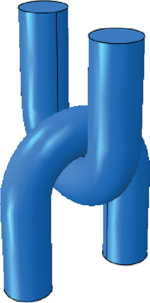
Figure 1: U-shaped ring model
3.2 Computational Domain and Boundary Conditions
The flow field was a cube, 500 mm × 500 mm × 500 mm (Fig. 2). ‘Inlet’ is set as ‘velocity-inlet’. ‘Outlet’ is set as ‘pressure-outlet’, and the pressure is 0 Pa. Because the wind velocity around U-shaped rings varied between 8–20 m/s [11], the wind velocity was set as 10 m/s, 20 m/s and 30 m/s, respectively. For discrete phase, the left surface of flow field was set as ‘surface injection’. The U-shaped rings surface were set as ‘wall’. The Erosion/Accretion model was selected. The discrete phase reflection coefficient is shown in Tab. 1.
Table 1: Discrete phase reflection coefficient
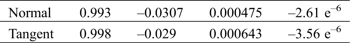
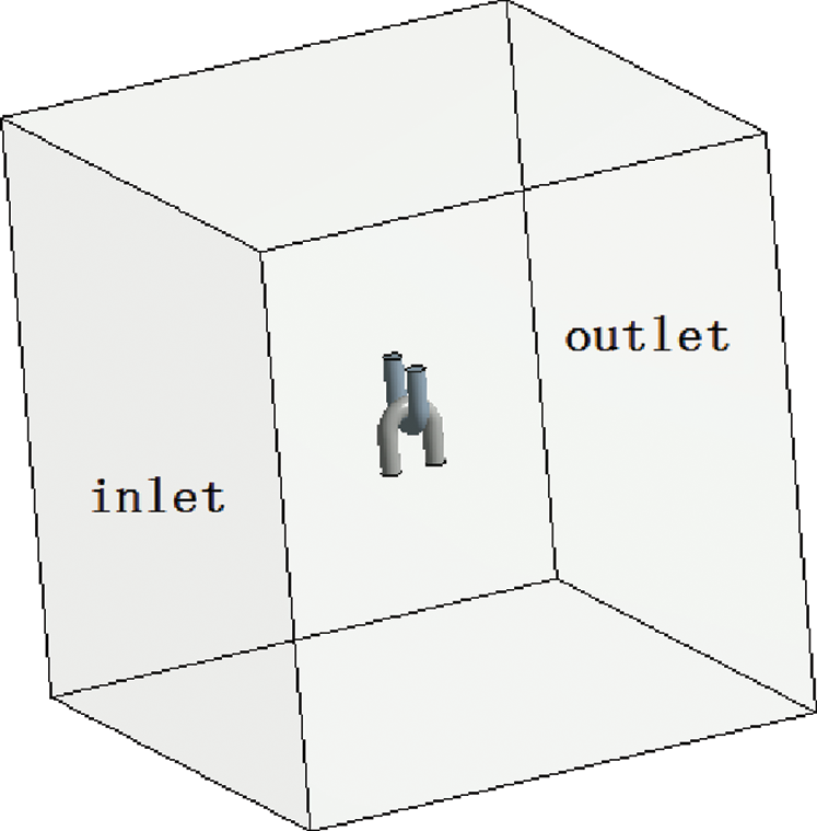
Figure 2: Flow field model
The sand density is 2650 kg/m, the specific heat capacity is 1230 j/kg k. The sand grain velocity was the same as the wind velocity, and the sand flow rate was 0.1 kg/s [17]. Due to the sand grain size was mainly concentrated between 0–0.25 mm, so the sand grain size was set to 0.25 mm [18]. Considering the effect of gravity.
The flow field was discretized by the tetrahedral mesh. Mesh thinning was performed on the boundary layer via the expansion layer. The expansion layer number was 5 and the growth rate was 1.2. The mesh independence tests were carried out through three different mesh sizes. In this paper, the wind velocity around the U-shaped ring is more concerned. Therefore, the influence sphere with different mesh sizes is used to refine the mesh, as shown in Tab. 2. The base size is the largest size of the mesh. The wind velocity was 20 m/s.
Table 2: Mesh sensitivity analysis
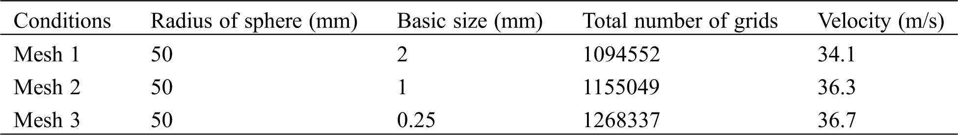
The accuracy of the numerical simulation is improved with the increasing mesh. Tab. 2 depicts that the relative error between Mesh 1 and the other two sets of mesh is larger, and the relative error between Mesh 2 and Mesh 3 is smaller [14]. Hence, Mesh 2 was selected on the premise of consideration of the calculation accuracy and calculation time. The specific mesh is shown in Fig. 3.
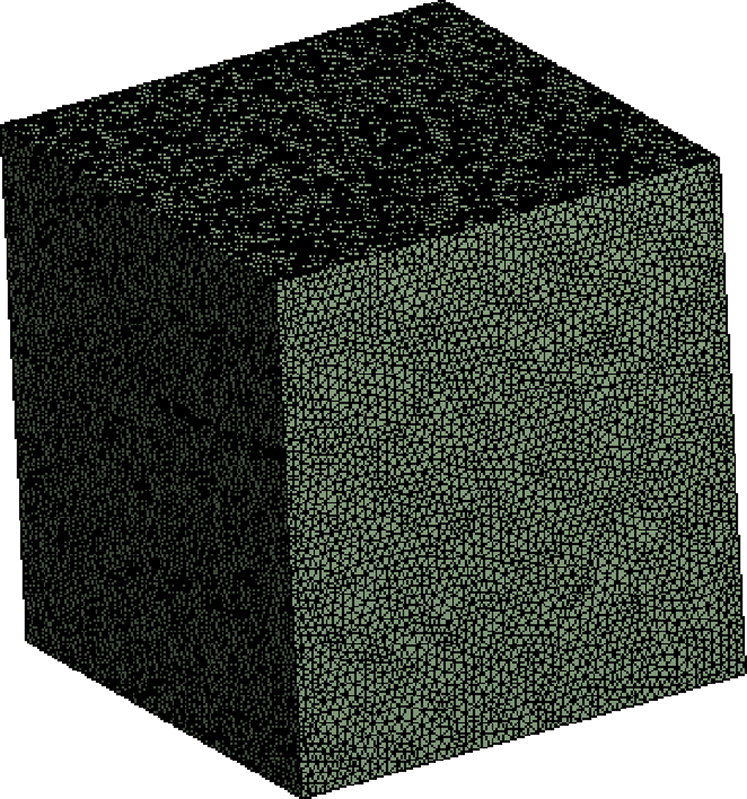
Figure 3: Grid division
4 Wind Field Simulation Results
The simulation result of wind pressure is shown in Fig. 4. It can be seen that the windward side of the U-shaped ring has the maximum wind pressure. Moreover, with the increase of wind velocity, the wind pressure increases rapidly, and the wind pressure at 30 m/s is about 8 times larger than that at 10 m/s. The negative pressure zone does not appear on the leeward side, but on both sides of the U-shaped ring. Under the same wind velocity, the value of negative pressure is greater than that of positive pressure zone, and the difference between the maximum value of positive and negative wind pressure becomes larger and larger with increasing wand velocity.
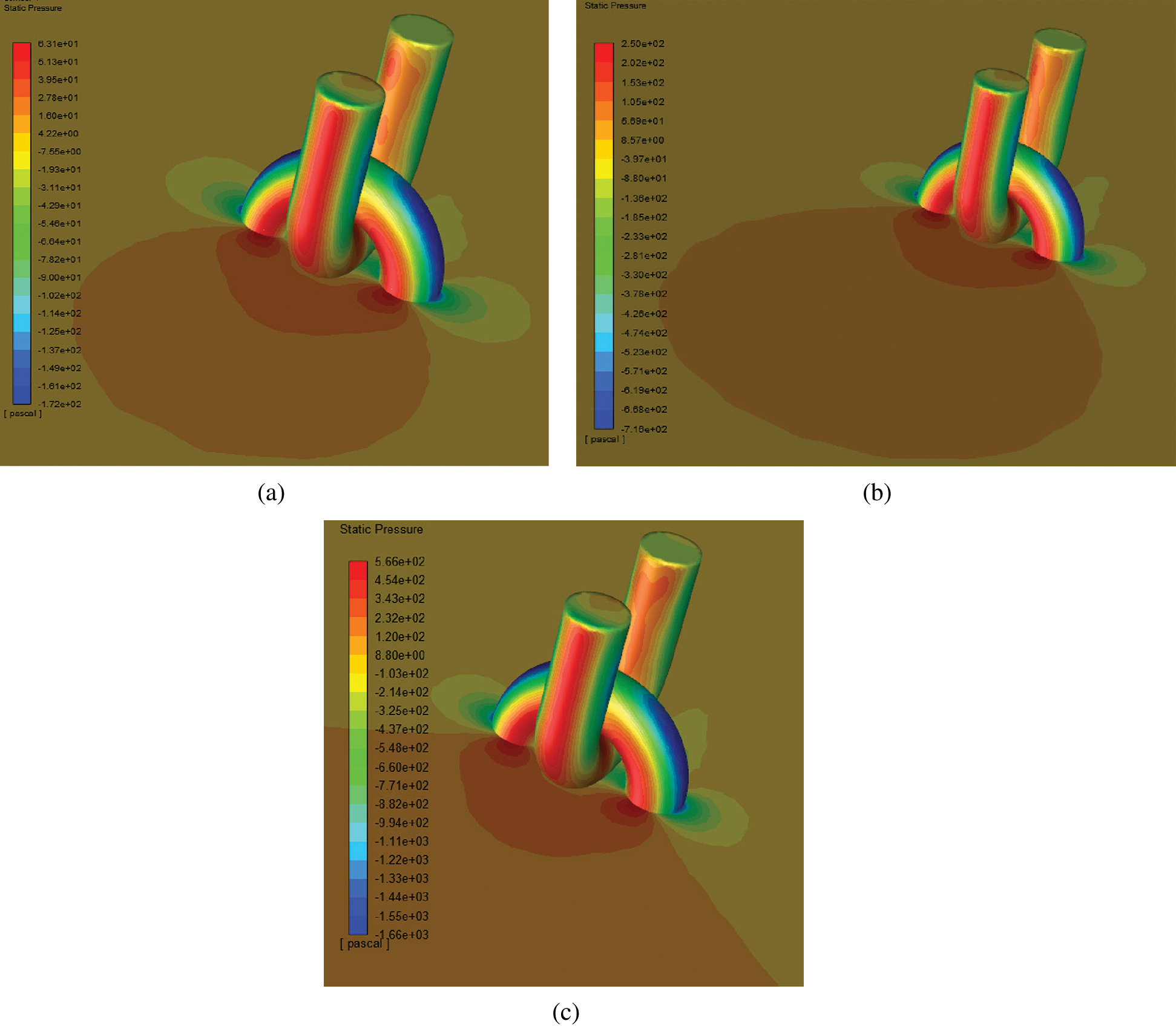
Figure 4: Wind pressure around U-shaped ring. (a) Wind velocity 10 m/s (b) Wind velocity 20 m/s (c) Wind velocity 30 m/s
The wind velocity around U-shaped ring is shown in Fig. 5. The maximum wind velocity appears on both sides of the U-shaped ring, and the maximum wind velocity is approximately 1.8 times higher than the input wind velocity. The position of maximum wind velocity is consistent with the position of minimum wind pressure. Because the maximum design wind velocity at the height of 10 meters for the transmission line is 42 m/s [19]. The input wind velocity was fitted linearly with the maximum wind speed around U-shaped ring, and the fitting results were shown as follows:
where x is the input wind velocity(m/s); y is the maximum wind velocity that can be achieved locally in the U-shaped ring(m/s).
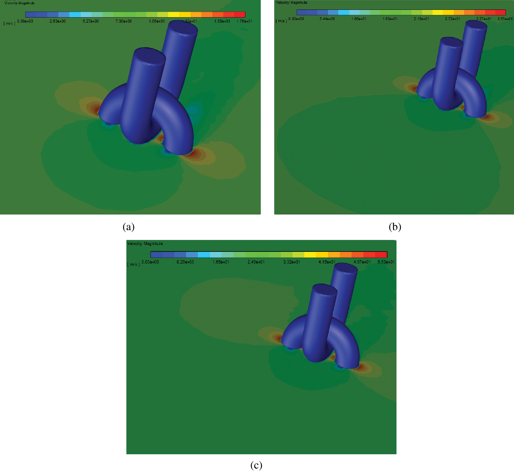
Figure 5: Wind velocity around U-shaped ring. (a) Wind velocity 10 m/s (b) Wind velocity 20 m/s (c) Wind velocity 30 m/s
The R value of linear fitting is 1, which indicates that the input wind velocity is completely linearly correlated with the maximum wind velocity around U-shaped ring. The maximum designed wind velocity of 42 m/s was put into the above equation, and the input wind velocity was 23 m/s. Therefore, when the wind velocity exceeds 23 m/s, the local maximum wind velocity near the U-shaped ring has exceeded the maximum design wind velocity. When the U-ring works for a long time with wind velocity greater than 23 m/s, it will cause the U-shaped ring to wear and fail prematurely.
5 Wind-Sand Two-Phase Flow Simulation
5.1 Wind Field Changes and Reasons
Euler-Lagrange approach was used to simulate the wind-sand field, and the incident velocity of the sand grains was set as 20 m/s. Fig. 6 shows the cross-sectional streamline diagram of the flow field and the vector diagram of the airflow cross-section. It can be seen that when the airflow does not contact the U-shaped ring, the airflow streamlines are parallel to each other. When the airflow touches the U-shaped ring surface, which produces flow around surface, and the airflow streamline also gradually change from slow flow to sharp flow [20]. The airflow presents an area with zero wind velocity on the leeward side of the U-shaped ring. Wind velocity disturbances are severe around the lower U-shaped ring and in the middle of the upper U-shaped ring (Fig. 6(b)). Combining with the Fig. 4, it can be seen that the airflow has the highest wind pressure on the windward side of the U-shaped ring. With the effect of the airflow, the magnitude and direction of the wind velocity change dramatically from the windward surface of the U-shaped ring to both sides, which results in the positive pressure zone from the windward surface gradually into the negative pressure zone on both sides.
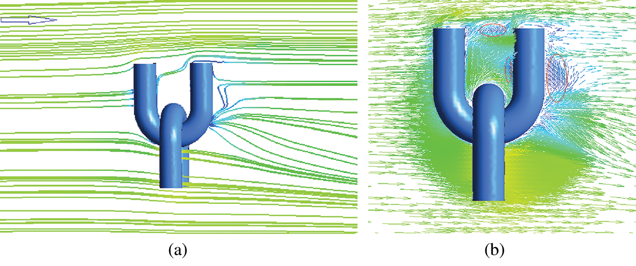
Figure 6: Streamline diagram of the flow field and vector diagram. (a) Airflow cross-section streamline diagram (b) Airflow velocity vector diagram
In order to explore the reason why wind velocity on the leeward side of the U-shaped is zero, observing the Fig. 7 that a vortex is generated in the red elliptical area. The cylinder Reynolds number is used to determine whether the vortex is a Kármán Vortex Street. The formula for calculating the Reynolds number is as follows [21]:
where
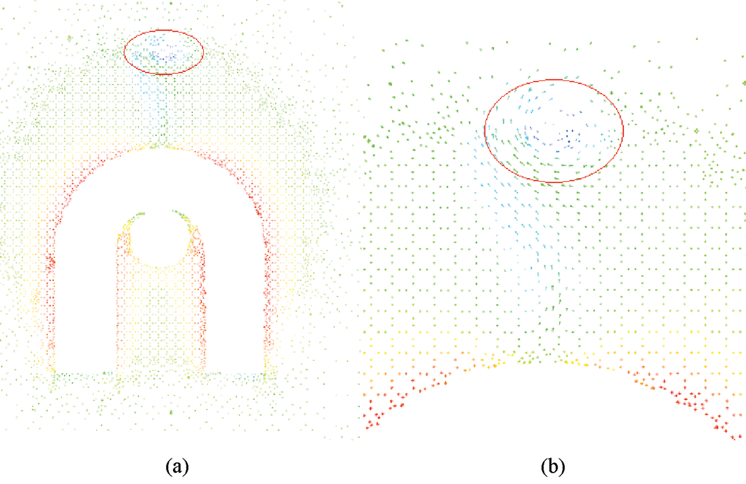
Figure 7: Cross-sectional velocity vector. (a) Airflow velocity vector diagram (b) Enlarged view of elliptic region
According to the above formula, Re = 2.8 × 10⁴, which satisfies the condition of existence of the cylindrical Kármán Vortex Street 47 < Re < 105. From the above analysis, it indicates that the region with zero wind velocity is caused by the whirl of airflow.
Combined with the above analysis, the reasons for the formation of the wind field around the U-shaped ring are explained in detail by observing Fig. 8. On the front view of flow field (Fig. 8(a)), the airflow is obstructed on the windward surface of the U-shaped ring, and the airflow velocity decreases. Subsequently, the airflow is divided into two parts. One part of the airflow flows to the cylindrical end surface of the U-shaped ring, and the other part flows to the outside of the bottom arc of the U-shaped ring. Then the airflow continues to move forward and encounters the incoming flow. The airflow inside the U-shaped ring is also divided into two parts. The airflow near the cylindrical end face of the U-shaped ring collide and intersect with the subsequent incoming flows, which results in a vortex near the end surface in the U-shaped ring, as shown in Fig. 7(a). The airflow near the bottom bend of the U-shaped ring collides with the cylinder end at the back of the U-shaped ring. One part moves upward around the cylinder end and intersects with the incoming flow. The other part flows along the U-shaped ring toward the contact part at the bottom bend to form a ‘semi-vortex’. When the airflow reaches the leeward side of the U-shaped ring, One part forms the reverse airflow flow to the leeward side of the U-shaped ring, resulting in a large vortex. The other part continues to move forward and enters the wake area. On the top view of flow field (Fig. 8(b)), the airflow encounters the obstruction of the U-shaped ring, the airflow velocity slows down. The airflow bypasses both sides of the U-shaped ring in a symmetric way and intersect with the incoming airflow, which causes local disturbance and increasing wind speed at the side of the U-shaped rings [22].
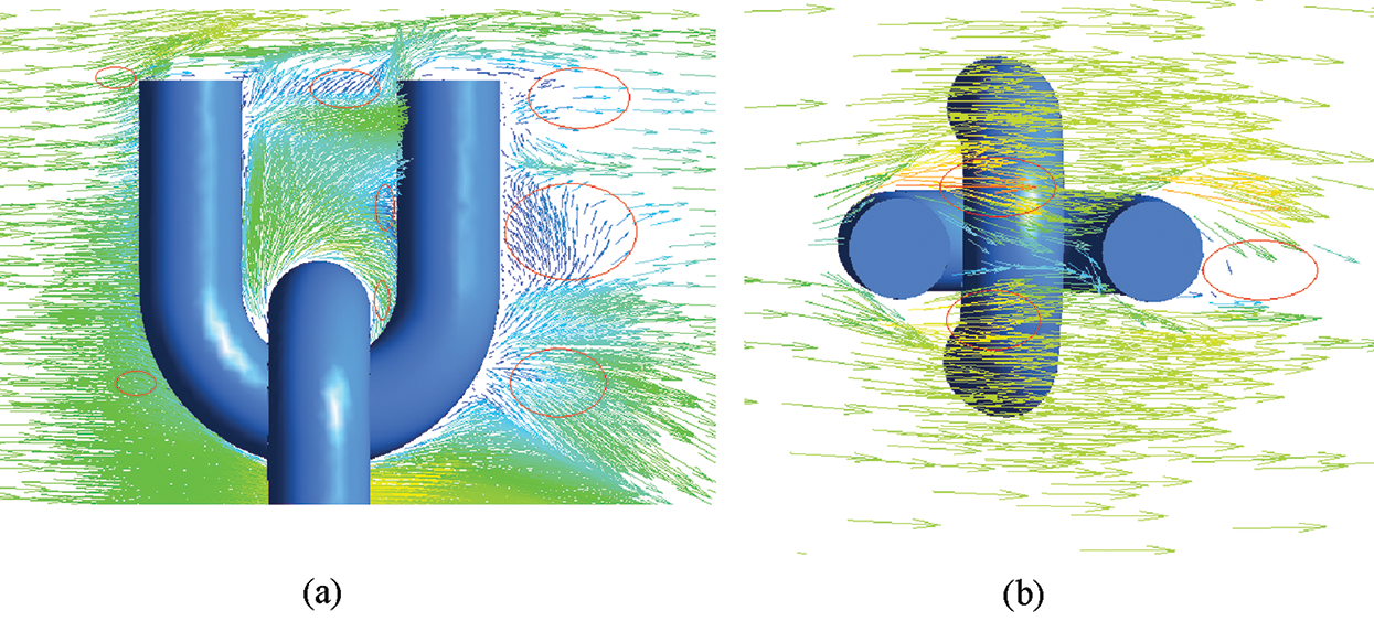
Figure 8: Velocity vector diagram of the flow field. (a) Flow velocity vector diagram of front view cross-section of flow field (b) Top view of flow field Cross-section flow velocity vector diagram
5.2 The Movement Regime of Sand Grains in Wind-Sand Field
By observing the Fig. 9, there are three movement regimes for the sand trajectory in wind-sand field. The first kind of sand grains are far away from the surface of the U-shaped ring. The sand grains are not affected by the change of the flow field on the surface of the U-shaped ring and fall along the parabola under the sand grains’ gravity (Fig. 10(a)). The second kind of sand grains are affected by the flow field on the surface of the U-shaped ring, but do not directly collide with the U-shaped ring. The trajectory of sand grains changes due to the effect of airflow, and local fluctuations occur during the falling process of sand grains. When the sand grains are far away from the surface of the U-shaped ring, sand grains still fall in a parabolic manner (Fig. 10(b)). The third kind of sand grains directly collide with the surface of U-shaped ring, which changes the movement direction of sand grains after bouncing off the surface (Fig. 10(d)).
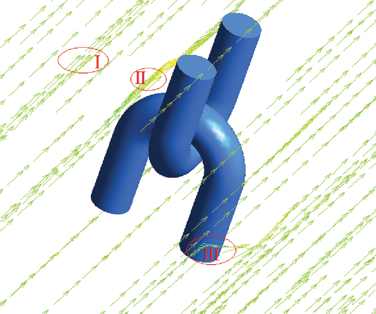
Figure 9: Sand grain velocity vector diagram
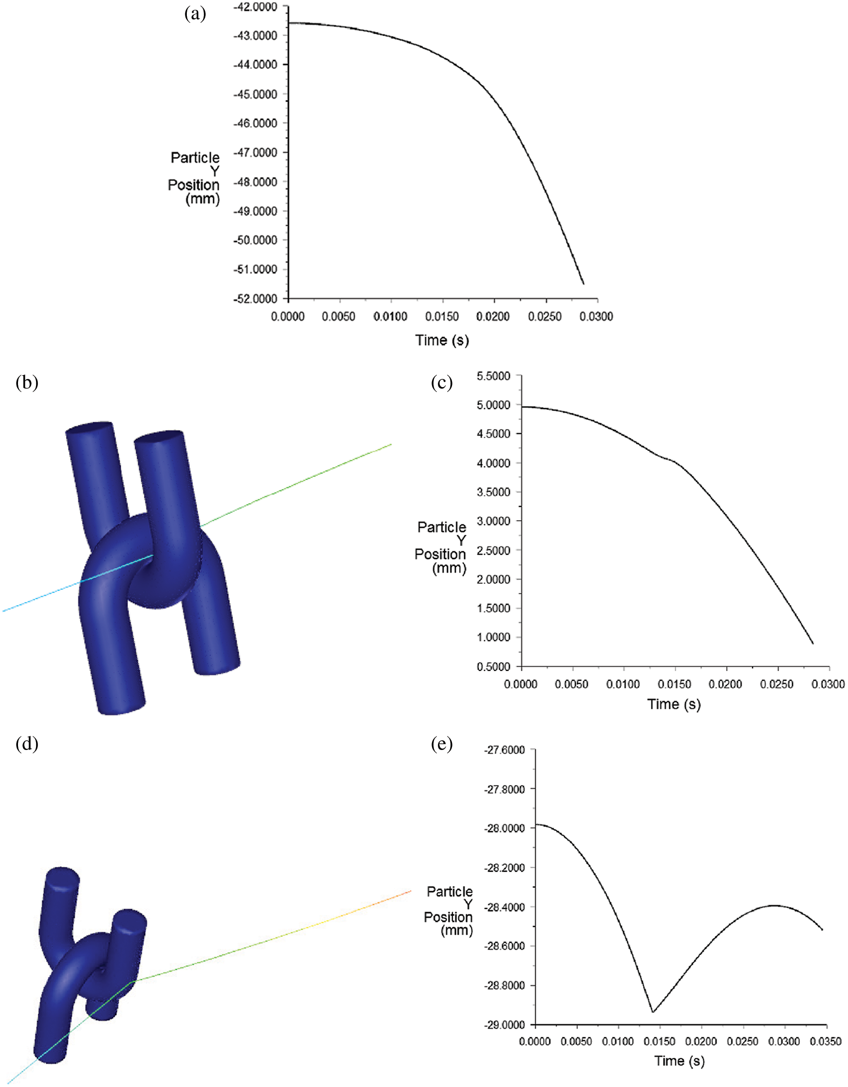
Figure 10: Sand movement mode. (a) The first pattern of sand grain fall (b) The second kind of sand trajectory (c) The second pattern of sand grain fall (d) The third kind of sand trajectory (e) The third pattern of sand grain fall
The main impacts on the U-shaped ring are the second and third sand trajectories. Stokes numbers in the flow field are often used to describe the follow ability of sand grains to the flow. When the Stokes number is large, the inertia of the sand particles plays a leading role, and the sand particles follow poorly. When the Stokes number is small, the sand particles follow better [23]. The formula for calculating sand Stokes number is as follows:
where V is characteristic flow velocity, V = 20 m/s; D is the characteristic value, D = 0.02 m;
It can be seen from the Fig. 6 that on both sides of the upper U-shaped ring, a ‘semi-vortex’ that flows to the contact part of the two U-shaped rings be generated. Sand grains with better follow ability will follow semi-vortex into the contact part of the two U-shaped rings and accelerate the wear failure of the U-shaped ring. For the third type of sand movement trajectory, on the one hand, the direct collision of sand grains will produce erosion on the surface of U shaped rings, which affects the service performance of the U-shaped ring. On the other hand, as shown in Fig. 11, the sand grains that collide with the contact area of the two U-shaped rings may be directly captured due to the fretting between the two U-shaped rings, which accelerates the wear failure process of the U-shaped rings.
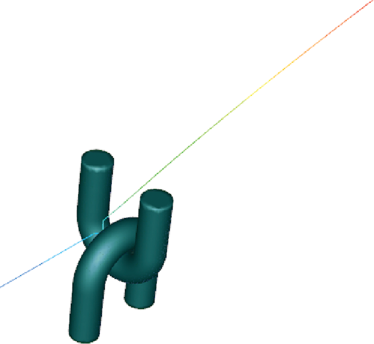
Figure 11: Trajectory diagram of sand grains colliding with U-shaped ring contact area
5.3 Sand Size that Flows to the Contact Areas of the U-Shaped Ring
As the wear progresses, the contact state between the two U-shaped rings would gradually change from point contact to surface contact. The increase in the contact area improve the ability of sand grains to follow the airflow into the contact area of the two U-shaped rings. The sand grains with smaller sizes may follow ‘semi-vortex’ into the contact area of the two U-shaped rings. Therefore, the sand grain sizes were selected to be 0.025 mm, 0.05 mm, 0.1 mm, 0.125 mm and 0.15 mm. The sand grain diameter range that can follow the airflow into the contact area of the two U-shaped rings was determined by the sand streamline diagram (Fig. 12). When the sand grain size is within 0–0.05 mm, the number of sand grains flowing into the contact area gradually increases with the increase of grain size. When the sand particle size is within 0.05–0.1 mm, the number of sand particles flowing into contact area doesn’t change much as the sand particle size increases. But the sand is getting closer and closer to the center of the U-shaped ring contact region. When the sand grain size is within 0.1–0.125 mm, the number of sand grains flowing into contact area gradually decreases with the increasing sand size. Therefore, when the sand size is less than 0.125 mm, the sand grains can follow the airflow into the contact area. Moreover, when the particle size is about 0.1 mm, the number of sand grains blown into the contact area of the two U-shaped rings is the largest, which is consistent with the conclusion of Deng et al. [5] that the U-shaped rings wear the most, when the particle size is 0.09–0.1 mm. As shown in Fig. 12(e), when the sand size is greater than 0.125 mm, the sand grains can’t follow the airflow into the contact area.
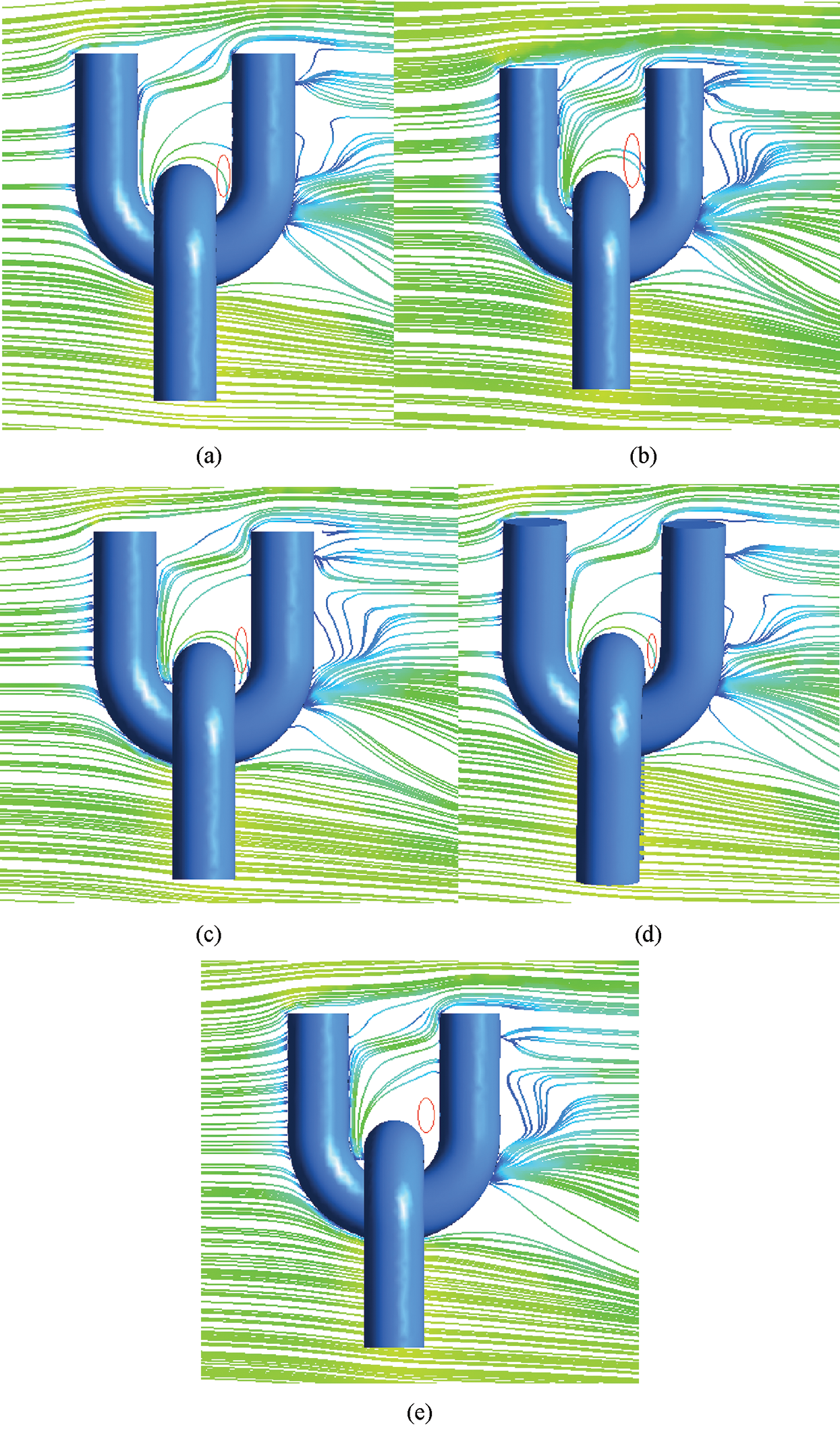
Figure 12: Streamline diagram of sand with different sizes (a) 0.025 mm (b) 0.05 mm (c) 0.1 mm (d) 0.125 mm (e) 0.15 mm
1. Under strong wind environment, the windward side of the U-shaped ring is positive pressure zone, and both sides of the U-shaped ring are negative pressure zones.
2. In the wind-sand field, the sand grains have three movement regimes. Sand grains not only collide with the U-shaped rings directly, but also enter the contact area between the two U-shaped ring to accelerate the wear and failure of the U-shaped rings.
3. Sand grains size in the range of 0–0.125 mm can follow the airflow into the contact area of the two U-shaped rings, and when the sand size is about 0.1 mm, the number of sand grains entering the contact area of the two U-shaped rings is the largest.
Funding Statement: This paper was supported by National Natural Science Foundation of China (51865055) and Tianshan Talents Plan of Xinjiang Autonomous Region of China (201720025)
Conflicts of Interest: The authors declare that they have no conflicts of interest to report regarding the present study.
1. Huang, Y. D. (2015). Study on the planning and some problems of Xinjiang 750 kV ultra-high voltage power grid. Beijing: North China Electric Power University. [Google Scholar]
2. Li, Q. (2013). Analysis and calculation of design wind speed for 750 kV transmission line from Urumqi to Hami. Electric Power Survey & Design, 2013(4), 27–30. [Google Scholar]
3. Shao, J. N., Wei, C., Wang, Y. (2016). Analysis and study of transmission line windproof measures in Xinjiang strong wind area. Journal of Henan University of Engineering (Natural Science Edition), 28(4), 45–48. [Google Scholar]
4. Yang, X. C. (2017). Research of transmission line electric power fittings wear in Xinjiang wind region. Urumqi: Xinjiang University. [Google Scholar]
5. Deng, H. M., Cai, W., Zhang, W., Xie, H., Zhang, L. et al. (2018). Sand erosion simulation experiments on link hardware of transmission lines: Mechanical property and microanalysis. High Voltage Engineering, 44(12), 3920–3928. [Google Scholar]
6. Zhao, J. P., Deng, H. M., Zhang, W., Zeng, W. J., Xie, H. et al. (2018). Sand erosion simulation experiments on link hardware of transmission lines: Test setting and corona analysis. High Voltage Engineering, 44(9), 2904–2910. [Google Scholar]
7. Wang, X. H., Li, X. M., Lu, P. P. (2020). Analysis of static and dynamic characteristics of U-shaped ring based on ANSYS-workbench. Journal of Xinjiang University (Natural Science Edition), 37(2), 242–247. [Google Scholar]
8. Lu, P. P. (2019). Research on wear behavior of transmission lines power fittings under strong wind environment. Urumqi: Xinjiang University. [Google Scholar]
9. Rawlins, C. B. (2000). The long span problem in the analysis of conductor vibration damping. IEEE Transactions on Power Delivery, 15(2), 770–776. DOI 10.1109/61.853018. [Google Scholar] [CrossRef]
10. Urchegui, M. A., Hartelt, M. (2008). Analysis of different strategies to reduce fretting wear in thin steel roping wires. Tribotest, 14(1), 43–57. DOI 10.1002/tt.52. [Google Scholar] [CrossRef]
11. Lu, X. (2013). Experimental research on transmission line wron in wind-sand two-phase flow. Beijing: North China Electric Power University. [Google Scholar]
12. Zhu, H. Y. (2015). FLUENT15.0 flow field analysis practical guide. Beijing: People Post Press. [Google Scholar]
13. Dai, Z., Li, T., Zhang, W., Zhang, J. (2020). Numerical study on aerodynamic performance of high-speed pantograph with double strips. Fluid Dynamics & Materials Processing, 16(1), 31–40. DOI 10.32604/fdmp.2020.07661. [Google Scholar] [CrossRef]
14. Li, G. (2020). Simulation of the thermal environment and velocity distribution in a lecture hall. Fluid Dynamics & Materials Processing, 16(3), 549–559. DOI 10.32604/fdmp.2020.09219. [Google Scholar] [CrossRef]
15. Cai, L., Lou, Z., Liu, N., An, C., Zhang, J. (2020). Numerical investigation of the deposition characteristics of snow on the bogie of a high-speed train. Fluid Dynamics & Materials Processing, 16(1), 41–53. DOI 10.32604/fdmp.2020.07731. [Google Scholar] [CrossRef]
16. Li, H., Yu, M., Zhang, Q., Wen, H. (2020). A numerical study of the aerodynamic characteristics of a high-speed train under the effect of crosswind and rain. Fluid Dynamics & Materials Processing, 16(1), 77–90. DOI 10.32604/fdmp.2020.07797. [Google Scholar] [CrossRef]
17. Zhao, J. P., Ai, H., Wang, X. X., Sun, Y. Q., Yan, Z. T. et al. (2018). Effects of wind-sand flow on wind load of conductors. Electric Engineering, 5, 14–16. [Google Scholar]
18. Jiang, F. Q., Li, Y., Li, K. C., Cheng, J. J., Xue, C. X. et al. (2010). Study on structural characteristics of gobi wind sand flow in 100 km wind area along Lan-Xin railway. Journal of the China Railway Society, 32(3), 105–110. [Google Scholar]
19. Meng, Y., Jia, Z. D., Zhu, Z. Y., Ma, G. X., Wang, X. L. et al. (2013). Study on failure of composite insulators used on transmission lines at “SanShiLi wind region” in Xinjiang. Environmental Technology, 31(1), 19–23. [Google Scholar]
20. Li, W. T., Jin, A. F., Li, H., Yang, S. Q. (2020). Numerical simulation study on erosion to high-speed trains by strong sand environment. Railway Locomotive & Car, 40(1), 13–18. [Google Scholar]
21. Lin, Y. C. (2015). Research on LGJ-400/50 ACSR surface erosion characteristics in wind sand environment. Beijing: North China Electric Power University. [Google Scholar]
22. Wang, J. C. (2019). Numerical wind tunnel simulation of high-rise buildings. Changchun: Jilin University of Architecture. [Google Scholar]
23. Araujo, A. D., Andrade, J. S., Jr, Maia, L. P., Herrmann, H. J. (2009). Numerical simulation of particle flow in a sand trap. Granular Matter, 11(3), 193–200. DOI 10.1007/s10035-009-0131-9. [Google Scholar] [CrossRef]
 | This work is licensed under a Creative Commons Attribution 4.0 International License, which permits unrestricted use, distribution, and reproduction in any medium, provided the original work is properly cited. |