Fluid Dynamics & Materials Processing

DOI: 10.32604/fdmp.2021.014249

ARTICLE

A CFD Study on a Biomimetic Flexible Two-body System

Jianxin Hu, Xin Huang and Yuzhen Jin*

Faculty of Mechanical Engineering and Automation, Zhejiang Sci-Tech University, Hangzhou, 310018, China
*Corresponding Author: Yuzhen Jin. Email: gracia1101@foxmail.com
Received: 13 September 2020; Accepted: 07 February 2021

1  Introduction

Fishes has developed excellent swimming skills to adapt environment through millions of years of evolution [1], therefore fish swimming can be a source of inspiration for the development of underwater vehicles [2,3]. Although the underwater submarine has good maneuverability [4], its propulsion efficiency can be further improved by bionic modeling. Bionic engineers have been working on the morphological characteristics and hydrodynamic performance of fish swimming for decades. In general, fish swimming is a process in which objects and fluids interact with each other. Most fishes swim with Body and/or Caudal Fin (BCF) pattern [5]. In this pattern, the tail of the fish swings and undulates regularly to create a series of vortex to gain thrust forward, while the body of the fish wobbles slightly to maintain stability [6,7].

The propulsion efficiency and performance of fish body is analyzed with certain kinematic parameters. Previous studies have indicated that the structure and stiffness of caudal fin play important roles [8–11]. Sfakiotakis et al. [7] concluded that the caudal fin provides 90 percent of the propulsion. Walker et al. [12] found out a better body fineness ratio can significantly reduce drag and improve swimming performance. Moreover, by studying the flow field pattern around fish body and fish tail, Zhao et al. [13] found that the separated caudal tail can greatly improve the propulsion performance. Li et al. [14] developed tree-like/structure model and serial-like/structured model to mimic fish undulation. By using several rigid elements to represent the flexible fish body, simple fish model can be built to explore the principle of fish swimming, and meanwhile the computation time is saved vastly.

Propulsive mechanism of single joint fish have been studied in the past by experiments and numerical simulation as well as flow around airfoils and cylinders [15,16], while there are still lots of morphological, behavioral and environmental complexities which may hinder researcher to reach the inherent mathematical principle [17–20]. In the present study, computational fluid dynamics (CFD) simulations are carried out to explore the fluid dynamic characteristics of a simplified fish model. To simplify the aforementioned serial-like/structured model, a single joint fish model which consists of fish body and caudal fin is built. In the past, relevant studies have been done in-depth on single-joint and double-joint robotic fish, and experiments have also verified the feasibility of this kind of model [21,22]. With different values of Strouhal number ( St ) and Reynolds number ( Re ), the model’s propulsive performance will be affected. St number is determined by inflow velocity, heave amplitude and frequency of caudal fin swing and Re number is decided by inflow velocity, body length and fluid viscosity. We aim to analyze the principle of anti-Kármán vortex and study how St and Re numbers affect the thrust force and propulsive efficiency by CFD simulation.

In this paper, fish model is presented and simplified and its kinematics is also described, followed by the description of the numerical method and the parameter setting in Section 2. To save computation time and increase computation accuracy, the grid independence is presented to choose the best model with suitable grid. The pressure contours and vortex structures are given to explore the principle of anti-Kármán vortex street in Section 3. Base on this, different conditions of fish swimming are simulated to analyze the effect of Strouhal number ( St ) on fish’s propulsive efficiency. Finally, the conclusions are summarized.

2  Methods and Model

2.1 Geometric Model

The geometric model in current study is two-dimensional. As shown in Fig. 1, this model is consisted of a fish body and a fish tail, and both of them can be either rigid or deformable. These elements are connected with one virtual hinge. At the hinge, there is only one degree of freedom of rotating motion about z axis. Prescribed rotation velocity can be provided at hinge so that the fish tail will rotate by the hinge.

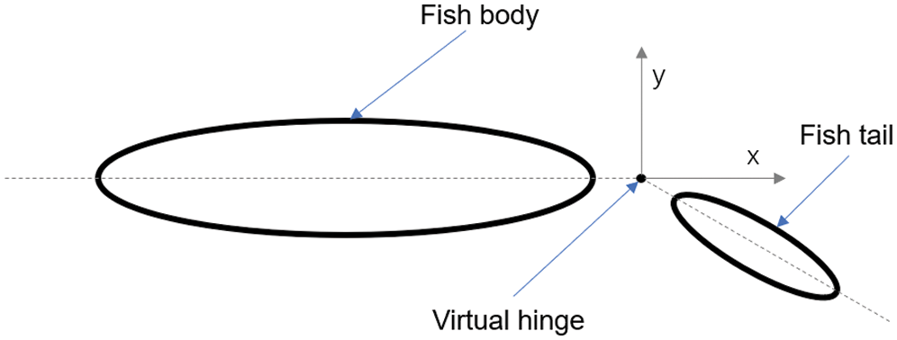
Figure 1: Two-segment fish model in current simulation

To reduce the amount of computation cost, we have simplified this simulation model, the caudal fin (fish tail) is considered as rigid rather than flexible and additional fins are neglected. In addition, three-dimensional (3-D) flow effects of the surrounding water are not considered.

2.2 Mathematical Model and Numerical Method

ANSYS Fluent 18.0 is used to carried out the simulation. The fluid motion is governed by incompressible continuity and moment equations as:

∇⋅u=0 (1)

∂u∂t+u⋅∇u=1ρ∇p+μρ∇2u (2)

where u is fluid velocity vector, p is fluid pressure, μ is fluid viscosity and ρ is fluid density. Two-dimensional (2-D) transient incompressible laminar flow is conducted.

The dynamic mesh feature is used with smoothing, layering and remeshing methods. The swing of caudal fin is realized by user-defined function (UDF). The fluid domain is set as 0.8 m × 1.5 m. The length of fish body and caudal fin are 0.06 m and 0.03 m, respectively, the whole fish is 0.093 m (including the gap between body and caudal fin). The geometry and mesh arrangement are shown in Fig. 2. The inlet boundary condition is set as velocity-inlet to control different velocities of inflow. The outlet boundary is set as outflow, and others are set as static wall surface.

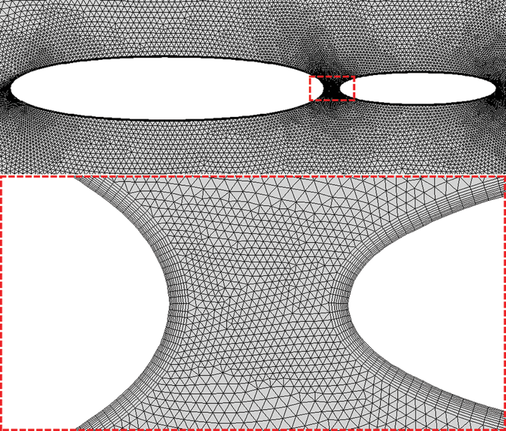
Figure 2: Body fitted mesh around current two-segment fish model

The fluid motion is solved with COUPLED algorithm as pressure-velocity coupling scheme to calculate non-stationary problems [14]. The first-order implicit transient formulation is adopted for the transient terms. For the spatial discretization option, the Least Squares Cell Based approach is employed for the gradient. To improve calculate accuracy, a second-order scheme is used for pressure interpolation and a second-order upwind scheme is selected for diffusive term discretization. In calculation setting, to avoid generating negative grid during the model movement, the time step is set as 0.001 s [13]. The max iteration number is 4000, and the convergence is assumed with all residual errors are less than 10−5 .

It is known that the caudal fin provides the major thrust force, and the flapping motion of caudal fin play a crucial role in propulsion performance. The kinematic motion of caudal fin is defined in UDF code. Generally, the motion of caudal fin can be described as a sinusoidal function:

ω(t)=ω0cos(ω1t+φ) (3)

θ(t)=ω0ω1sin(ω1t+φ) (4)

In the above Eqs. (3) and (4), ω(t) and θ(t) are the angular velocity and rotating angle of the midline of caudal fin, respectively; ω0ω1 is the maximum rotating angle, where ω0 defines the maximum angular velocity of the midline of caudal fin and ω1 is the angular frequency; φ is a phase angle.

2.3 Definition of Parameters

The length of the entire fish is L, and the fish body length and caudal fin length are c1 and c2 respectively. The inflow velocity is U0 .

When the fish-like model is swinging, there are two vital nondimensional parameters under consideration, i.e., the Strouhal number ( St ) and Reynolds number ( Re ), which are defined as follows:

St=2hfU (5)

Re=ρLUμ (6)

where f is the swimming frequency (in Hertz), h is heave amplitude and equal to the sinusoidal value of the maximum swing angle of the caudal fin in y -direction. ρ is fluid density, and μ is dynamic viscosity. Here, St number presents the relation between the caudal fin motion and free stream velocity [23] and Re number defines the ratio of inertial force to viscous force in fluid motion.

The propulsive efficiency can be expressed as the following equation [24]:

η=C¯tC¯ip¯ (7)

To study the efficiency ( η ) of the caudal fin we need to know the mean thrust coefficient ( Ct ), mean lift force coefficient ( Cl ), mean input power coefficient ( Cip ), and they are defined as follows:

Ct=Fx12ρU2L,Fx=1T∫0T⁡X(t)dt (8)

Cl=Fx12ρU2L,Fy=1T∫0T⁡Y(t)dt (9)

Cip=P12ρU3L,P=1T[∫0T⁡Y(t)dhT(t)dtdt+∫0T⁡M(t)dθ(t)dtdt] (10)

where Fx is periodic average value of the force component X(t) of entire fish body in x -direction, Fy is periodic average value of force component Y(t) of entire fish body in y -direction, T is flapping period, and P is periodic value of input power. We can compute the efficiency by these equations above.

2.4 Validation

A validation case was carried out on a 2-D foil model as shown in Fig. 3, which has been reported in our previous work [25]. The 2-D foil model undergoes a prescribed heave motion while freely movement in x-direction [26]. The foil motion is also realized with dynamic mesh feature and inhouse developed UDF code. The induced velocity (non-dimensionlized as Reu) with heave frequency (non-dimensionlized as Refr) is compared to Alben & Shelly’s results [26], and it shows good results especially in low Refr region.

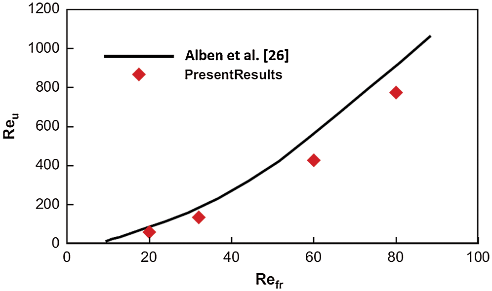
Figure 3: Comparation with previous work [26]

3  Results

3.1 Mesh Independence Study

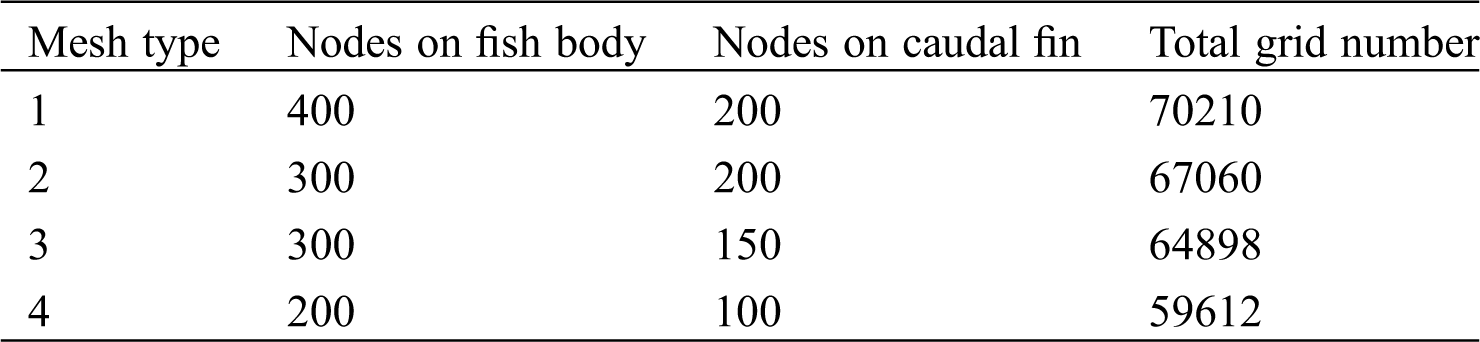
The quality of mesh has great effects on the time consuming and accuracy of the simulation. In this model, the parameters are: f=0.5Hz , U=0.008m/s , h=0.0315m (corresponding maximum swing angle is 30°). Different density of mesh has been built for the mesh independence study. Tab. 1 shows the number of element node on fish body and caudal fin, in which Mesh 1 and Mesh 2 are the finest meshes.

Table 1: Information of different mesh types of fish model

10 oscillating cycles are simulated and each cycle has 2000 time-steps to make sure it is short enough to meet the calculation accuracy required by dynamic mesh. Figs. 4 and 5 show the time histories of the Cl and Ct of this model in one single period. By comparing these results, we can conclude that the calculation results of different meshes have a good match. Among these calculation results, mesh 2 fits well with mesh 1 (with most elements).

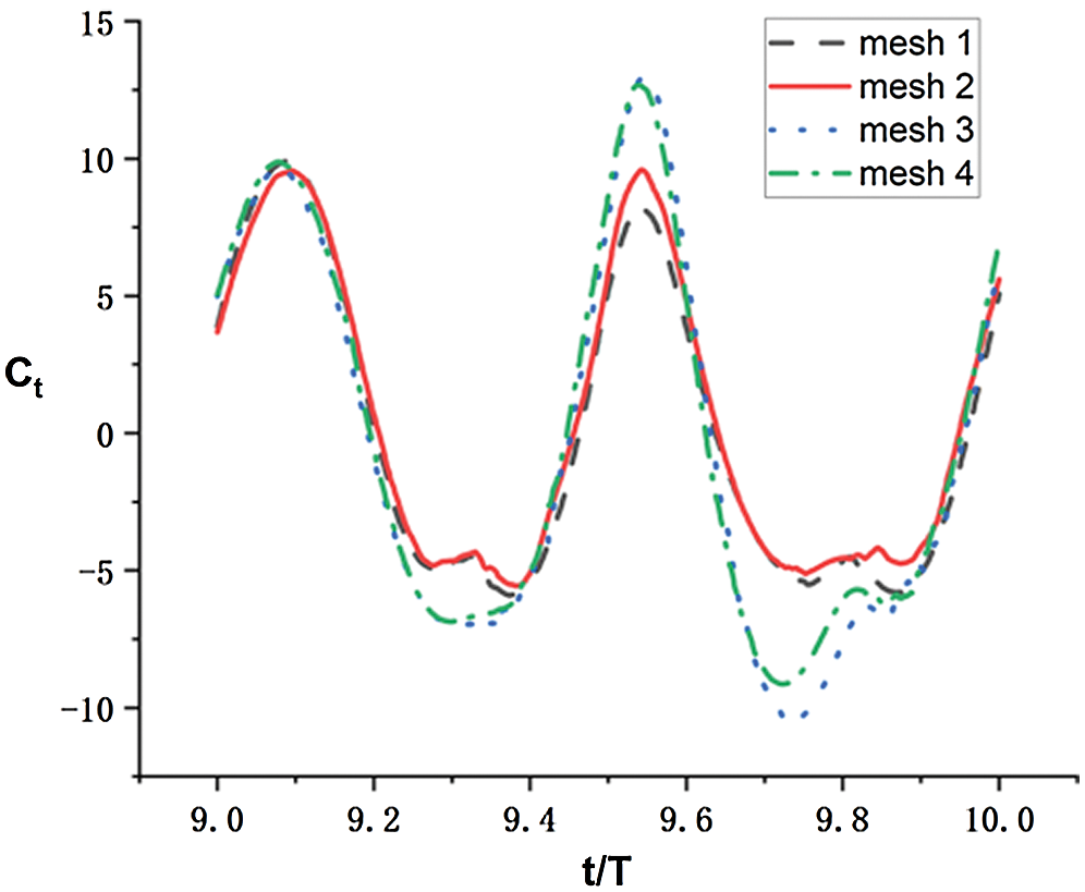
Figure 4: Comparation of thrust coefficient ( Ct ) for different meshes

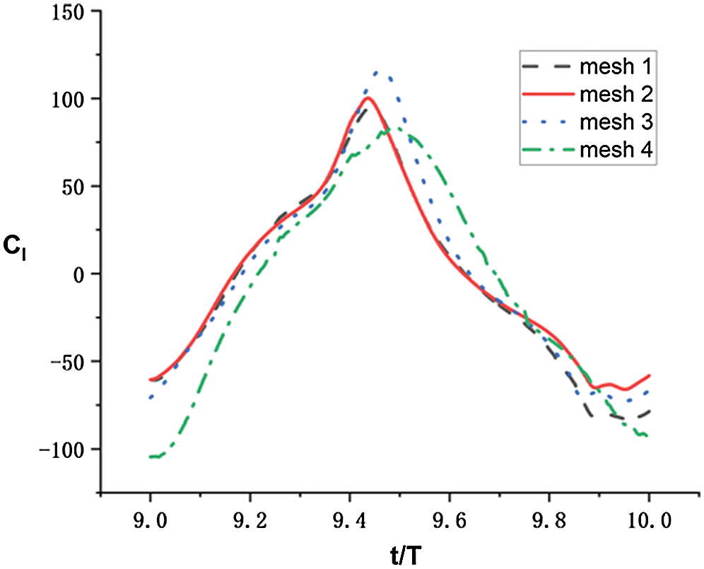
Figure 5: Comparation of lift coefficient ( Cl ) for different meshes

3.2 Principle of Anti-Kármán Vortex Street

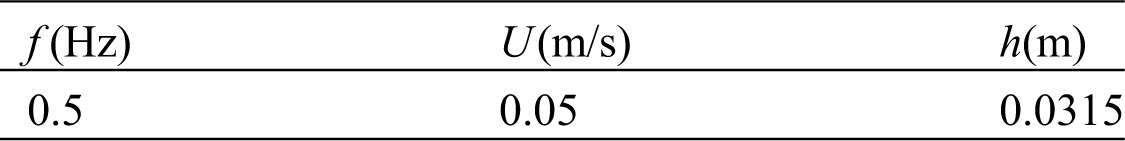
In the subsection, we will first explain the principle of fish swimming with respect to anti-Kármán vortex street. A working condition based on Eqs. (3) and (4) is chosen to study this principle, Tab. 2 shows the selection of parameters.

Table 2: Parameter selection of current simulation

Figs. 6 and 7 respectively show the pressure contour and vortical contour around swimming fish model. The flow structures are detailed as follows:

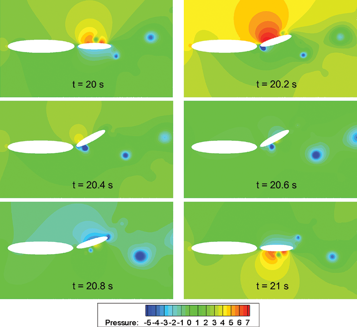
Figure 6: Pressure contours around the two-segment fish model at different time instances

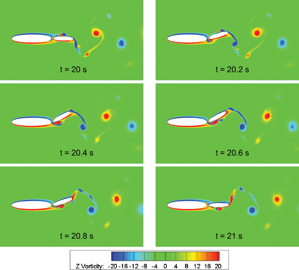
Figure 7: Vorticity contours around the two-segment fish model at different time instances

At t = 20 s, this model is swinging forward, and the caudal fin is at its starting position. In this movement, the caudal fin rotates around the virtual hinge to push the fish body forward in the negative direction of the x-axis. Due to the fish tail swing, there is a high-pressure zone on the upside of the caudal fin, and a low-pressure zone on the underside due to existing lower pressure. At this time instance, there are two tail vortexes behind the caudal fin.

During t = 20.2 s–20.4 s, the caudal fin is swinging up. The fluid pressure on the underside of the caudal fin continued to decrease, and began to move backward. The upper high-pressure region is largest at t = 20.2 s, then it will begin to shrink.

After that, the caudal fin moves to the maximum swing position. The low-pressure region on the upside of the caudal fin turns to be the largest, and the high-pressure region has been weakened. Then the caudal fin starts to swing back, the low-pressure region on bottom of the caudal fin becomes weak, and formed a high-pressure region beside the low-pressure region.

During t = 20.6 s–20.8 s, the low-pressure region of the caudal fin continues to be weakened. The upside of caudal fin began to form a low-pressure region. Then it continues to expand and to move to the end of caudal fin.

At t = 21 s, the caudal fin is back to the initial position. The low-pressure region moves downward from caudal fin and formed a tail vortex.

Moreover, during t = 20 s–20.4 s, the caudal fin is swinging counterclockwise. The underside of the caudal fin formed a low-pressure region and expanded continuously. As the caudal fin keeps swinging to the maximum swing angle, the high-pressure region on the upside of caudal fin continues to weaken at the maximum swing angle. During t = 20.6 s–21 s, the caudal fin is swinging clockwise. Its upside forms a low-pressure region and it is kept expanding. At the same time, the underside forms a high-pressure region. When it near to initial position, the new vortex sheds off. It can be seen from Fig. 7, during the fish swing, it generates two vortexes in a cycle. When caudal fin swings counterclockwise, it will form a tail vortex rotating clockwise. When it swings clockwise, there will be a tail vortex rotating counterclockwise. This is the principle of anti-Kármán vortex street, and fishes can swim forward because the generation of tail vortex produce the forward thrust.

3.3 Effects of Strouhal Number and Reynolds Number

The principle of fish swimming has been explored, then we are going to find out how different parameters affect the thrust of fish swimming and the efficiency. In this subsection, effects of St and Re numbers are investigated.

Choosing different inlet velocity of flow, we can obtain several conditions (cases) with different Re numbers. Firstly, in this part we mainly explored how do Re number and St number (determined by different inflow velocity) effect fish swimming based on current two-segment fish models. Tab. 3 shows the parameter selections of this study in which five different conditions are considered. Relevant results are shown in Figs. 8–11.

Table 3: Parameter selections for five conditions with different Re numbers

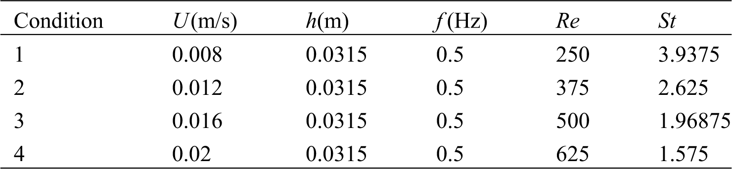
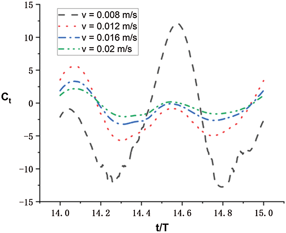
Figure 8: Thrust coefficients in a single period of the fish model for conditions with different Re number

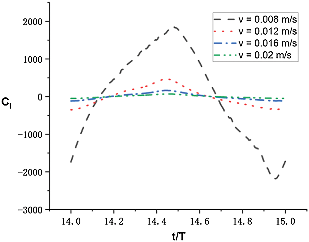
Figure 9: Lift coefficients in a single period of the fish model for conditions with different Re number

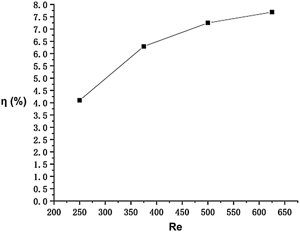
Figure 10: Propulsive efficiencies of the fish model for conditions with different Re number

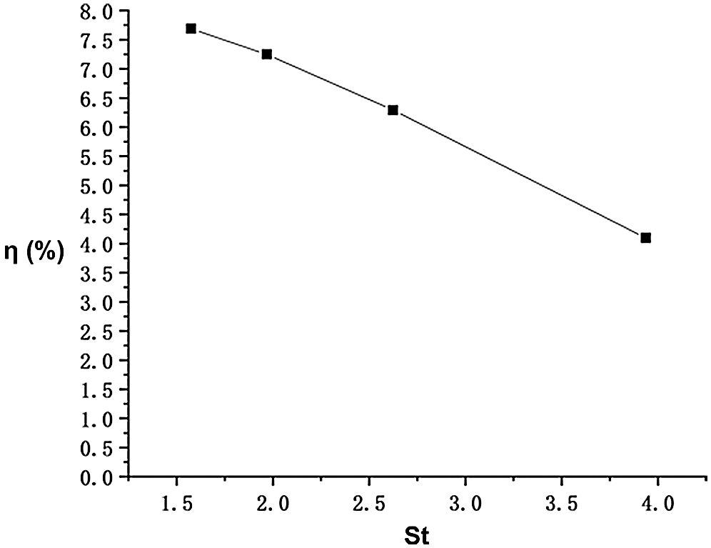
Figure 11: Propulsive efficiencies of the fish model for conditions with different St number based on different inflow velocity

We can find from the results that the thrust coefficient Ct increases when the velocity of flow decreases. When the Re is in the range of 375–625 or St is in the range of 1.575–2.625, it has weak influence on instantaneous Cl . However, the Cl changes drastically with lower Reynolds number. Therefore, the fish is affected by greater lift force at a relatively low Re (less than 375) or high St (larger than 2.625). With the relatively lager Re or less St , the fish body swims more stably. The efficiency of fish swimming increases and the trend turns weaker as the Re increases and it will approach to the maximum value of 8% when Re reaches 625. As the inflow velocity decreases, St gradually increase. The efficiency decreases linearly with increase of St.

Secondly, in this part we mainly explored that how St number affects fish swimming performance by changing the frequency or heave amplitude of caudal fin swinging. Parameters for cases with different St number based on variation of flapping frequency are given in Tab. 4, and relevant results are shown in Figs. 12–14.

Table 4: Parameter selections for six conditions with different St numbers by changing flapping frequency

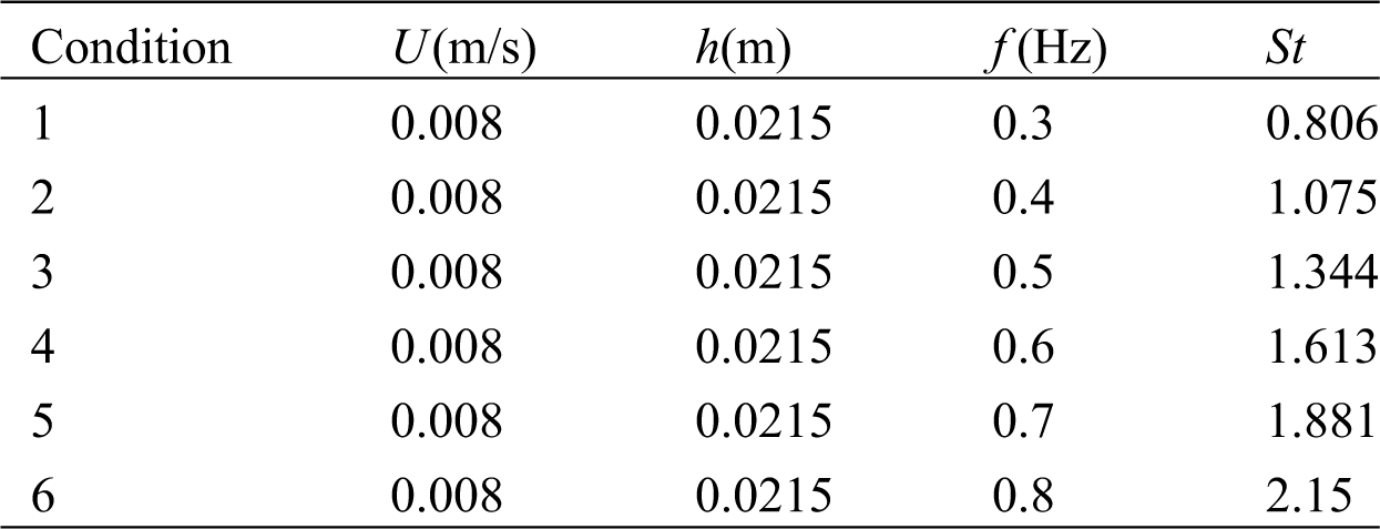
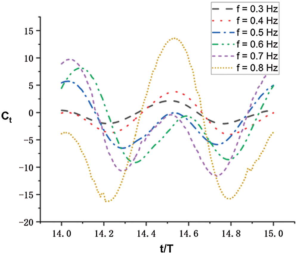
Figure 12: Thrust coefficients in a single period of the fish model for conditions with different St number based on different flapping frequencies

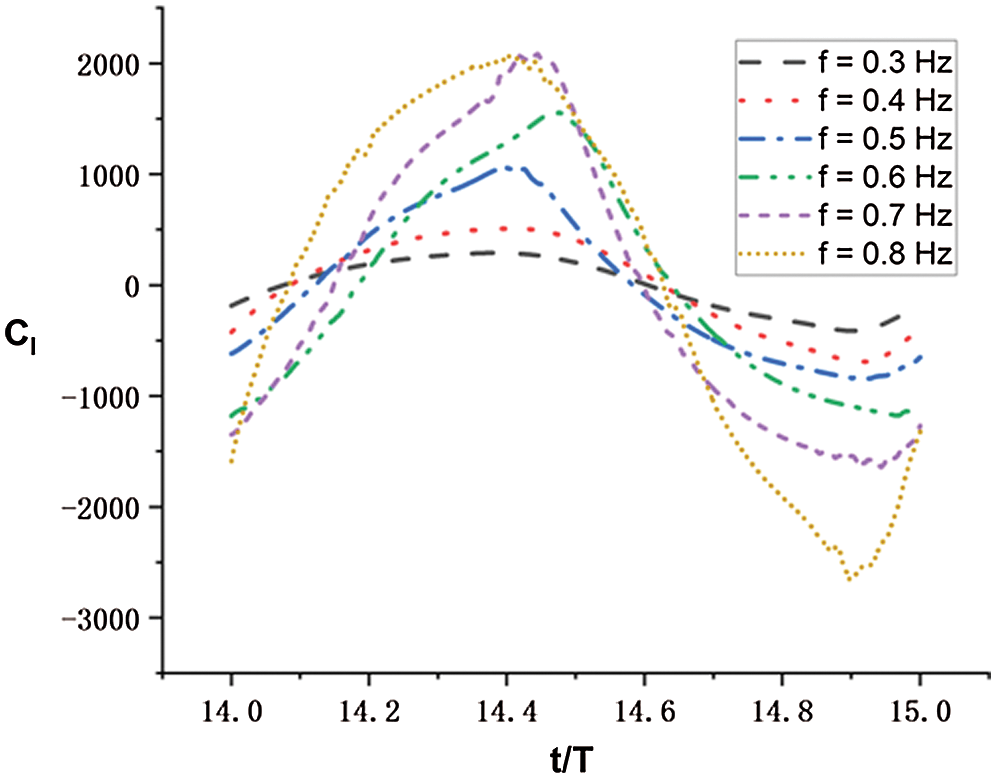
Figure 13: Lift coefficients in a single period of the fish model for conditions with different St number based on different flapping frequencies

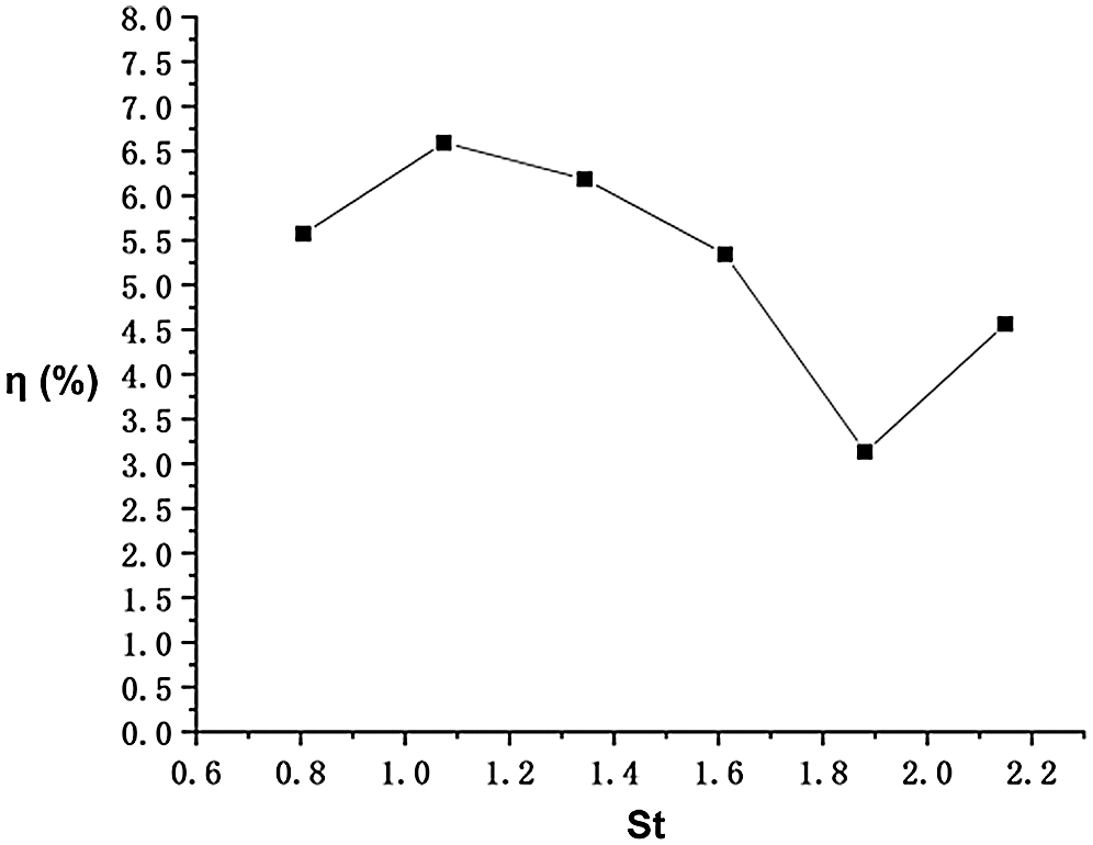
Figure 14: Propulsive efficiencies of the fish model for conditions with different St number based on different flapping frequencies

Moreover, cases with a larger heave amplitude are also studied, and the parameters for these cases are given in Tab. 5, and relevant results are shown in Figs. 15–17.

Table 5: Parameter selections for seven conditions with different St by changing flapping frequency, the heave amplitude is set as 0.0405 m

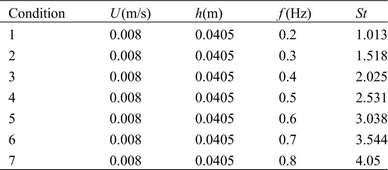
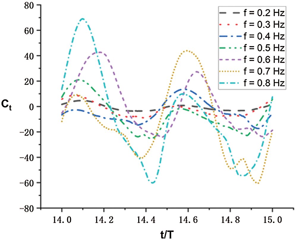
Figure 15: Thrust coefficients in a single period of the fish model for conditions with different St number based on different flapping frequencies

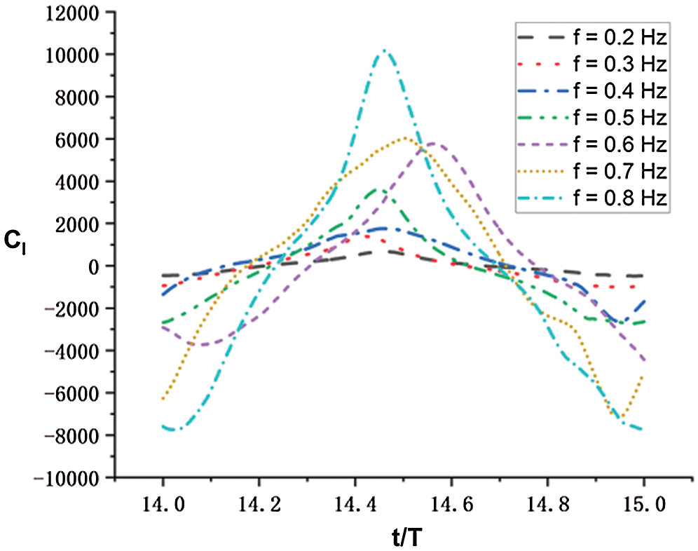
Figure 16: Lift coefficients in a single period of the fish model for conditions with different St number based on different flapping frequencies

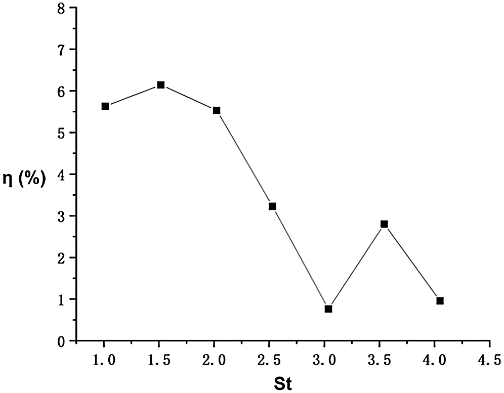
Figure 17: Propulsive efficiencies of the fish model for conditions with different St number based on different flapping frequencies

To obtain different St number by only changing the frequency of caudal fin swinging, we got the instantaneous Ct and Cl results. According to the results presented above, we can draw a conclusion that when heave amplitude is constant, Ct and Cl of fish mode will be larger with a higher frequency. This model has relatively higher efficiency when St number ranges from 1.0 to 2.0. When the caudal fin has large heave amplitude (0.0405 m), the efficiency of fish swimming decreases more sharply than small heave amplitude (0.0215 m) cases. It indicates that if the fish want to have high efficiency, it needs to swing its caudal with low frequency and swing angle.

In the following, we consider cases with different St number by changing the heave amplitude and two categories are employed with different flapping frequencies, i.e., f = 0.4 Hz and f = 0.8 Hz. Relevant parameters are given in Tabs. 6 and 7 respectively with corresponding results shown in Figs. 18–20 and Figs. 21–23.

Table 6: Parameter selections for six conditions with different St by changing heave amplitudes, the flapping frequency is set as 0.4 Hz

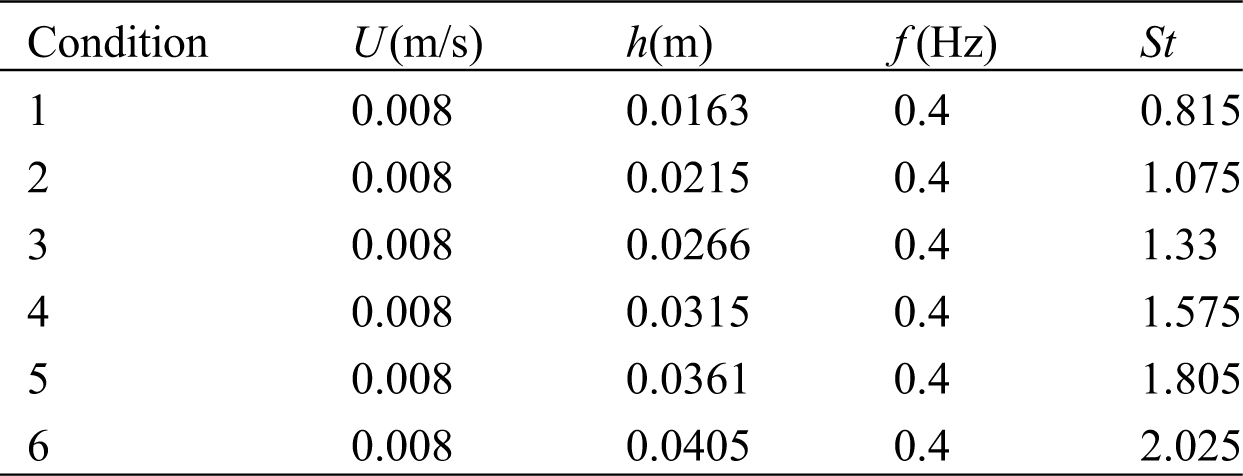
Table 7: Parameter selections for seven conditions with different St by changing heave amplitudes, the flapping frequency is set as 0.8 Hz

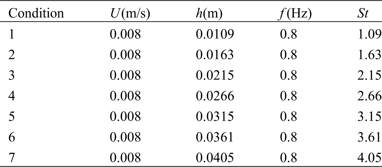
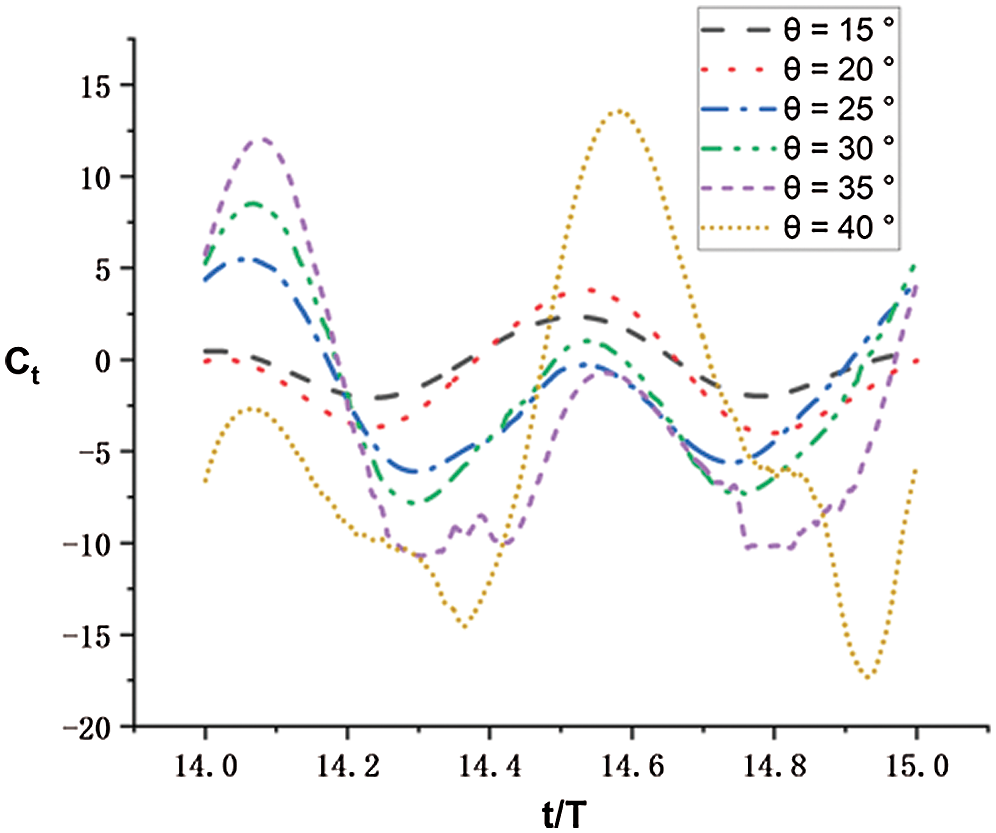
Figure 18: Thrust coefficients in a single period of the fish model for conditions with different St number based on different heave amplitudes

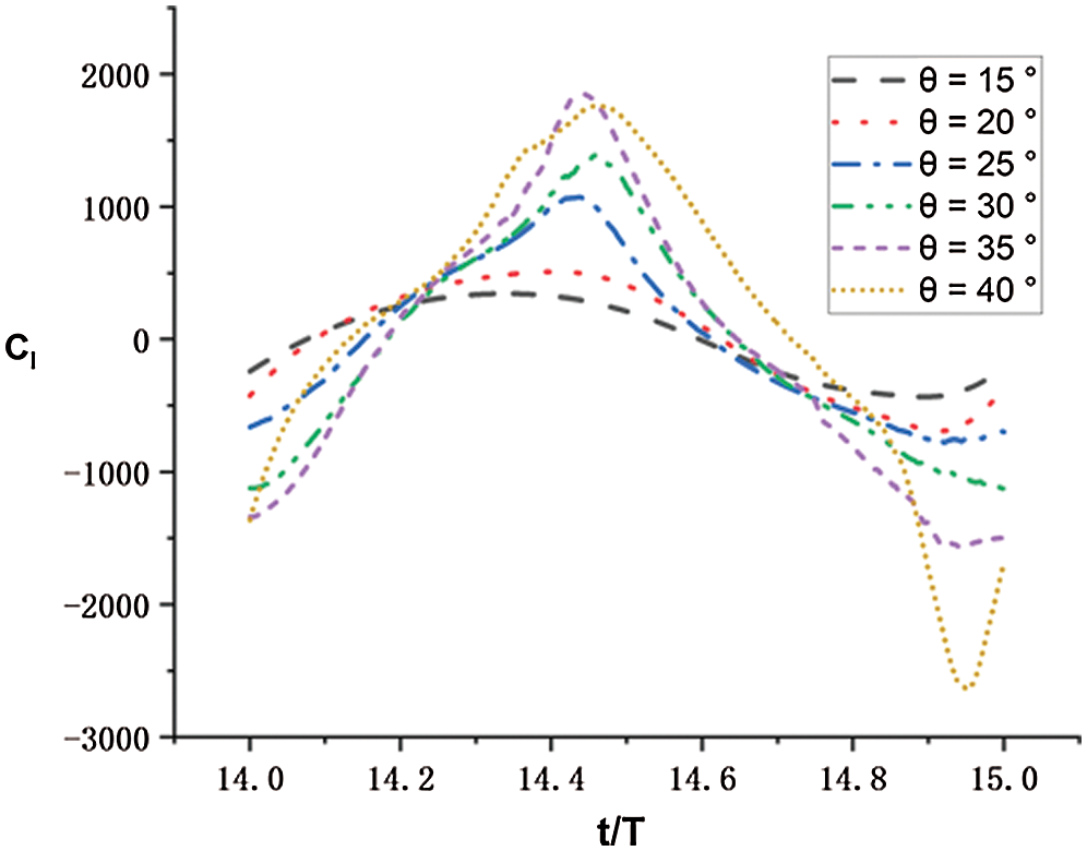
Figure 19: Lift coefficients in a single period of the fish model for conditions with different St number based on different heave amplitudes

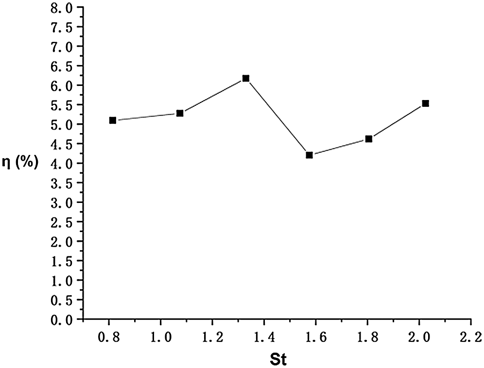
Figure 20: Propulsive efficiencies of the fish model for conditions with different St number based on different heave amplitudes

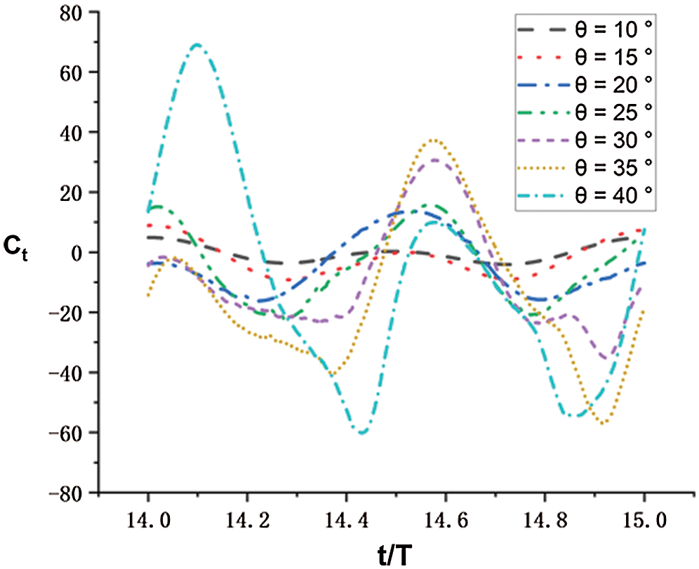
Figure 21: Thrust coefficients in a single period of the fish model for conditions with different St number based on different heave amplitudes

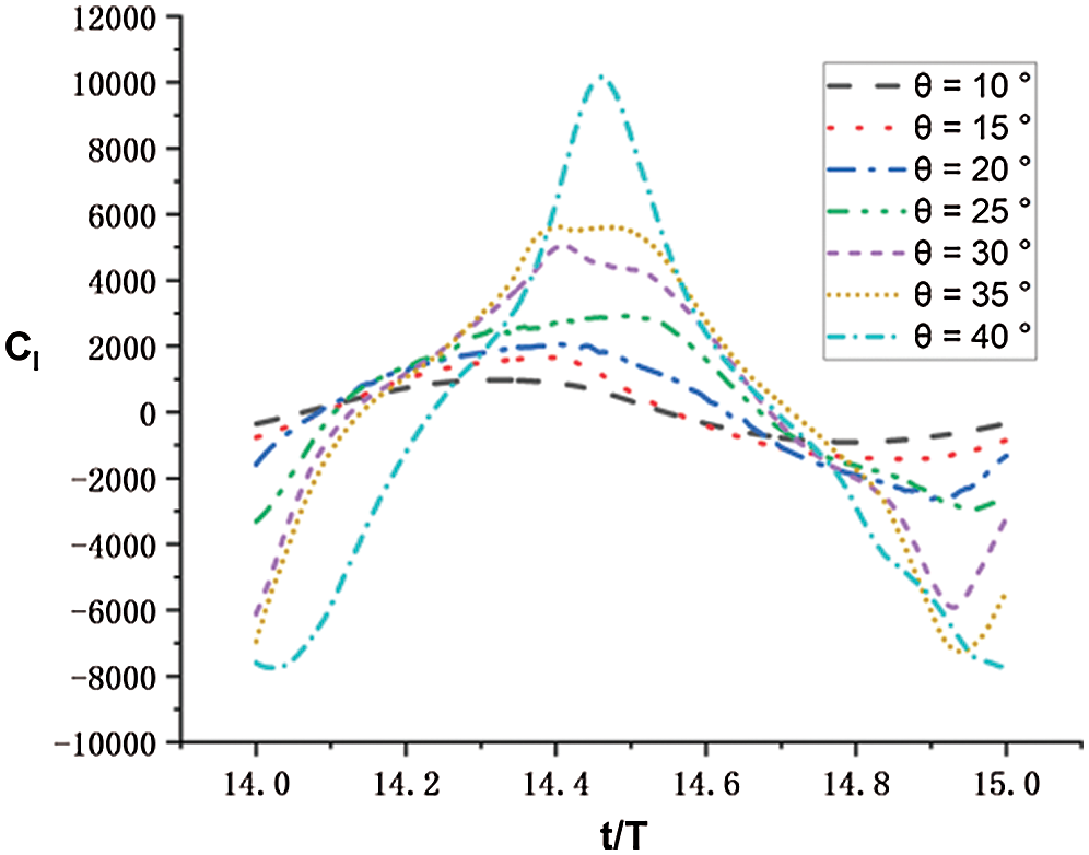
Figure 22: Lift coefficients in a single period of the fish model for conditions with different St number based on different heave amplitudes

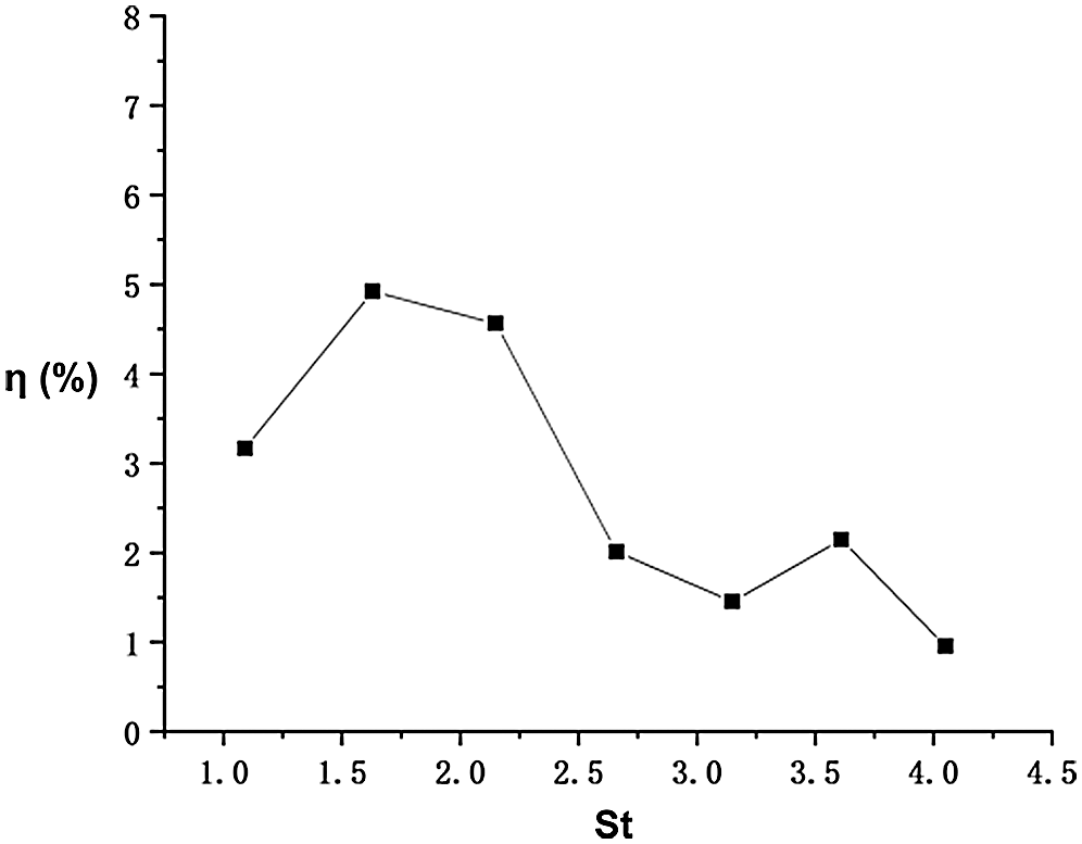
Figure 23: Propulsive efficiencies of the fish model for conditions with different St number based on different heave amplitudes

Above results are obtained by changing the heave amplitude of the caudal fin. We can find that if the heave amplitude increases, the Ct and Cl of fish model also increase. Therefore, in order to have a higher swimming efficiency, in these conditions, the St number with the range from 1.7 to 2.3 is preferable. Increasing heave amplitude has limited influence on fish swimming with low swinging frequency (0.4 Hz). However, if caudal fin has higher frequency (0.8 Hz), the efficiency will drop when heave amplitude is larger than 0.0215 m. By analyze how heave amplitude affect the swim efficiency, we can derive a similar conclusion like the tendency of swing frequency effect, that is, lower heave amplitude and swing frequency can improve fish propulsion efficiency.

4  Conclusion

In the present study, a single joint fish model was employed to explore the fish swimming performance. Using a simple fish model for numerical simulation, the mechanism of fish body swimming is explored. By analyzing the pressure contour and vorticity contour of the flow of fish swimming, it is concluded that caudal fin swing generates anti-Kármán vortex to push fish body to swim forward. In order to study how the fish swimming is affected by the Re and the St numbers, a series of working conditions (cases) are investigated and analyzed. We can draw a conclusion that fishes can obtain higher efficiency when they swim with lower heave amplitude and frequency. The Ct and Cl increase with the increasing of Re and the St numbers, and the optimal St number for propulsive efficiency is obtained under a certain range of fish tail swing frequency. By using a fairly basic and simplified model to analyze swimming mechanism of fish and its influencing factors, in may provide some reference for the efficiency optimization of single joint underwater robotic fish or other vehicles.

In this paper, with a two-dimensional biomimetic model to represent the cross-section of a fish, the flow field characteristics and the influence of non-dimensional parameters are studied. However, this paper is limited to computing resources, it has not been explored further with a three-dimensional model. In the future, the deficiencies in this area are expected to be solved and the fish propulsion mechanism will be improved in other aspects.

Funding Statement: This research was funded by the National Natural Science Foundation of China, Grant Nos. 51906224 and 51976200.

Conflicts of Interest: The authors declare that they have no conflicts of interest to report regarding the present study.

This work is licensed under a Creative Commons Attribution 4.0 International License, which permits unrestricted use, distribution, and reproduction in any medium, provided the original work is properly cited.