Fluid Dynamics & Materials Processing

DOI: 10.32604/fdmp.2021.012741

ARTICLE

A Combined Numerical-Experimental Study on the Noise Power Spectrum Produced by an Electromagnetic Sensor for Slurry Flow

Song Gao1,*, Xin Jin1 and Qiaohong Liu2

1College of Agricultural Equipment Engineering, Henan University of Science and Technology, Luoyang, 471023, China
2School of Medical Instruments, Shanghai University of Medicine and Health Sciences, Shanghai, 201318, China
*Corresponding Author: Song Gao. Email: gaosongsan@163.com
Received: 11 July 2020; Accepted: 07 February 2021

1  Introduction

1.1 Overview of Slurry Noise of Electromagnetic Flow Sensor

The advantage of electromagnetic flow sensor is simple structure, large measurement range, high measurement accuracy, good corrosion resistance, low requirement on velocity distribution, reliable use, convenient maintenance, long life, etc. Therefore, for slurry fluid with difficult flow measurement, electromagnetic flow sensor is the most widely used flow meter [1], such as iron ore pipeline transportation flow measurement [2–5], coal water slurry and pulp flow measurement [6–10], deep-sea mining slurry transportation [11] and so on. However, when using electromagnetic flow sensor to measure slurry fluid, there is a problem that the measurement signal is interfered by slurry noise, which leads to errors in the measurement results. Therefore, the purpose of this paper is to study the characteristics of slurry noise and provide some theoretical basis of solving the problem of slurry noise.

The output signal of the electromagnetic flow sensor used for measuring slurry fluid will frequently jump, which is shown as a random large jump signal. This phenomenon is called slurry noise [12–15]. The typical waveform of flow velocity signal measured by electromagnetic flow sensor for water and slurry is shown in Fig. 1.

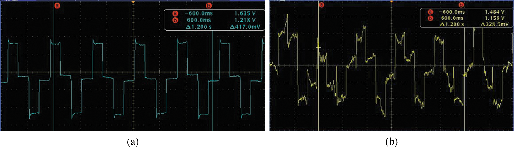
Figure 1: The flow rate induced potential signal waveform of the electromagnetic flow sensor. (a) Measurement waveform of the water; (b) Measurement waveform of the slurry

Fig. 1 shows the flow rate induced potential signal of electromagnetic flow sensor displayed by oscilloscope. The fluid measured by the electromagnetic flow sensor is water and slurry fluid, with the average flow velocity of 4m/s , the rectangular three-valued waves excitation is adopted by electromagnetic flow sensor, the excitation frequency is 3.125 Hz , and excitation current with positive-zero-negative-zero positive rule changes is adopted. In terms of measurement waveform, the Fig. 1a is the waveform of the water measured by electromagnetic flowmeter, and the Fig. 1b is the waveform of the slurry fluid measured by electromagnetic flowmeter. By comparing the Fig. 1a with Fig. 1b, it can be clearly seen that the measurement waveform has a large random potential interference in the measurement of slurry fluid, which manifests a large frequent jumping phenomenon, and it is the interference of measurement signal is affected by slurry noise. Shercliff [12] pointed out the reason of slurry noise: the slurry noise generates because of the solid particles collided with the surface of measuring electrode during the measurement of liquid-solid two-phase fluid. The analysis of the following: due to the corrosion of electrolyte, an oxide film will be formed into the surface of the measuring electrode of the electromagnetic flow sensor when it comes into contact with the measured fluid, during the formation process of oxide film, polarization voltage is generated between metal and electrolyte. If the materials of the two measuring electrodes are the same, polarization voltage will become a common mode interference voltage with equal polarity and amplitude. When the solid particles of liquid-solid two-phase flow fibers or hits the surface of electrode, the thin oxide film on the electrode surface is pulled or scratched, and the broken oxide film needs to be regenerated. During the process of reforming the oxide film, the polarization voltage between the electrode and the fluid changes suddenly. If there is a difference between the surface states of the two measuring electrodes, polarization common mode interference will become differential mode interference. Therefore, the large fluctuation appears in the electrode measurement signal, which leads to the appearance of slurry noise. Literature [16] points out that the collision of solid phase particles of measuring electrodes of electromagnetic flow sensor results in slurry noise, which will adversely to affect the measurement accuracy of the electromagnetic flow sensor. The above research reveals the causes of slurry noise, and shows that when applied to slurry measurement, it is inevitable that the measurement signal of electromagnetic flow sensor will be interfered by slurry noise. Because the installation position of the measuring electrode of the electromagnetic flow sensor is near the pipe wall, the collision of solid particles with the electrode can be obtained by studying the flow state and flow field distribution of slurry fluid near the pipe wall in the sensor measuring pipe. Literatures [17–21] shows that, based on the existing research on fluid boundary layer theory and CFD (computational fluid dynamics) theory, it is efficient and easy to obtain the flow field parameters near the pipe wall by numerical method. Therefore, in this paper, we will use the combination of numerical method and experiment to obtain slurry fluid parameters.

1.2 Research Status of Slurry Noise

Studying the characteristics of slurry noise and taking measures to reduce or eliminate the influence of slurry noise on measurement is currently hot topics in the research field of electromagnetic flow sensors, relevant scholars and technical workers have done a lot of research on the slurry noise problem of electromagnetic flow sensors and the solutions to the slurry noise.

The research of literatures [6,22–29] shows that slurry noise is a kind of random signal and has the property that the power spectral density is inversely proportional to the frequency, which is approximately 1/f. These studies believe that the power spectrum of the slurry noise has 1/f characteristic, and the slurry noise belongs to 1/f noise. Literatures [22–28,30,31] adopts various digital signal processing methods to solve the interference of slurry noise of electromagnetic flow sensor on measurement signals, and has achieved good results. These studies mainly reveal the 1/f characteristic of slurry noise power spectrum, and according to the 1/f characteristic of slurry noise, the influence of slurry noise on the output signal of electromagnetic flowmeter is solved by increasing excitation frequency. In essence, these methods all use signal processing to solve the slurry noise problem. However, this method has limitations, because the excitation frequency can not be increased without restriction, and too high excitation frequency will lead to poor stability of zero point of electromagnetic flow sensor.

If the sensor structure is optimized according to the flow field characteristics of slurry fluid, so as to reduce the number of collisions between solid particles of slurry fluid and electrodes per unit time, the problem of slurry noise can be well solved. According to the above ideas, we try to study the influence of slurry velocity and concentration distribution on slurry noise, which provides a theoretical basis for optimizing the sensor structure.

1.3 Characteristics and Research Status of 1/f Noise

Slurry noise belongs to random noise, and its power spectrum has 1/f characteristic, so the power spectrum model of slurry noise can be established by establishing 1/f noise model. At present, there are many achievements in the study of 1/f noise characteristics and simulation methods. Keshner [32] proposed that the random fluctuation phenomenon with the inverse ratio of power spectral density to frequency is called 1/f noise, and 1/f noise is a random process. Broadly speaking, if the power spectral density has a random fluctuation property that decreases with increasing frequency and increases with decreasing frequency, it can be called 1/f noise. van der Ziel et al. [33,34] classifies 1/f noise into basic and non-basic 1/f noise. Wornell et al. [35–37] gives a quasi-1/f signal generation theorem and a method to generate 1/f signals in a certain frequency range. Literatures [38,39] points out that 1/f noise belongs to pink noise in colored noise, and studies the method of simulating 1/f noise by computer, but the method of generating 1/f noise in these methods is too complex and requires a large amount of calculation. With the wide application in engineering field, using software to simulate physical phenomena has become an efficient research and experimental means. At present, using Matlab software to simulate 1/f noise is a more convenient method. The specific process is: design a digital filter, then use white noise as the input signal, and get 1/f noise through the filter. The DSP (Digital Signal Processor) toolbox of Matlab provides a digital filter for generating 1/f noise. Only by modifying the parameters of the filter, the required 1/f noise signals with different power spectral densities can be conveniently obtained, and unwanted signal components can be filtered by windowing.

Because the random signal can not be described by a mathematical formula, the characteristics of slurry noise signal can only be studied by analyzing the power spectrum. Its characteristics can only be studied by analyzing the power spectrum of the random signal. In the paper, the power spectrum of slurry noise is simulated by Matlab, and influence of slurry velocity and concentration on power spectrum of slurry noise is analyzed, which provides a certain theoretical basis of the research and development of electromagnetic flow sensor for slurry flows measurement. Based on the 1/f characteristic of the power spectrum of slurry noise, we directly call the 1/f noise program with the DSP toolbox of Matlab, and through modifying the parameters, the generated 1/f noise power spectrum graph is close to the real slurry noise power spectrum graph.

2  Simulation of Slurry Noise Power Spectrum

2.1 Simulation Principle of Slurry Noise Power Spectrum

Assuming that the solid particles impacting the electrode within a certain time t is a white noise sequence U(n) , σU2 is the variance of white noise sequence, the intensity of U(n) is 10lg⁡σU2 , it can be seen that the size of the variance σU2 of U(n) is related to the size of the number s of solid particles. Obviously, the number of solid particles colliding with the electrode in unit time is proportional to the product of the flow rate V and the volume concentration Cs of solid particles, if V or Cs increases, σU2 increases. On the contrary, if V or Cs decreases, σU2 decreases.

On the basis of the 1/f characteristic of the power spectrum of slurry noise, power spectrum X(n) can be generated by simulation, and X(n) is a sequence with 1/f characteristic. As long as an appropriate IIR (Infinite Impulse Response) filter H(z) is designed and white noise sequence with constant variance is taken as input, a standard 1/f noise sequence X(n) can be obtained by passing U(n) through H(z) , where the transfer function of filter can be obtained according to the characteristics of 1/f noise:

H(jω)=1jω=1ωe−j(π/4) (1)

or

H(s)=1s (2)

In this way, IIR digital filter H(z) can be seen as a process in which the electrodes of electromagnetic flow sensor are collided by solid particles of slurry fluid. If Cs or V of the measured slurry fluid changes, the number of solid phase particles impacting the measuring electrode in unit time will change accordingly, and σU2 will change accordingly. So the 1/f noise sequence X(n) also changes with the variance of U(n) . By comparing and analyzing the changes of X(n) , the characteristics of noise changing with the flow velocity and solid particle concentration can be obtained.

2.2 Simulation Implementation of Slurry Noise Power Spectrum of Electromagnetic Flow Sensor

The measurement pipeline and two-dimensional cross-section model of electromagnetic flow sensor are shown in Fig. 2.

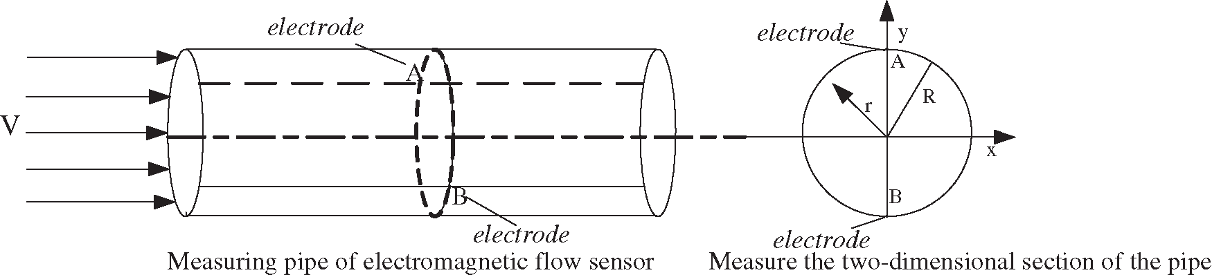
Figure 2: Schematic diagram of electromagnetic flow sensor measuring pipe and two-dimensional section

As shown in Fig. 2, the radius of two-dimensional section of the pipe measured by the electromagnetic flow sensor is R , and the distance from any point on the pipe section to the central position of the pipe section is r , A and B are the measuring electrodes of the electromagnetic flow sensor. The fluid fills the pipe, and V is the fluid flow velocity.

The installation structure of the electrode of the electromagnetic flow sensor is shown in Fig. 3.

Figure 3: Installation structure of electromagnetic flowmeter measuring electrode. 1-Nut; 2-Washer; 3-Wiring block; 4-Insulation lining; 5-Electrode; 6-Metal conductor; 7-Spring washer; 8-Insulation sleeve

Divide the pipe in accordance with the radial position r/R , as showed in Fig. 4.

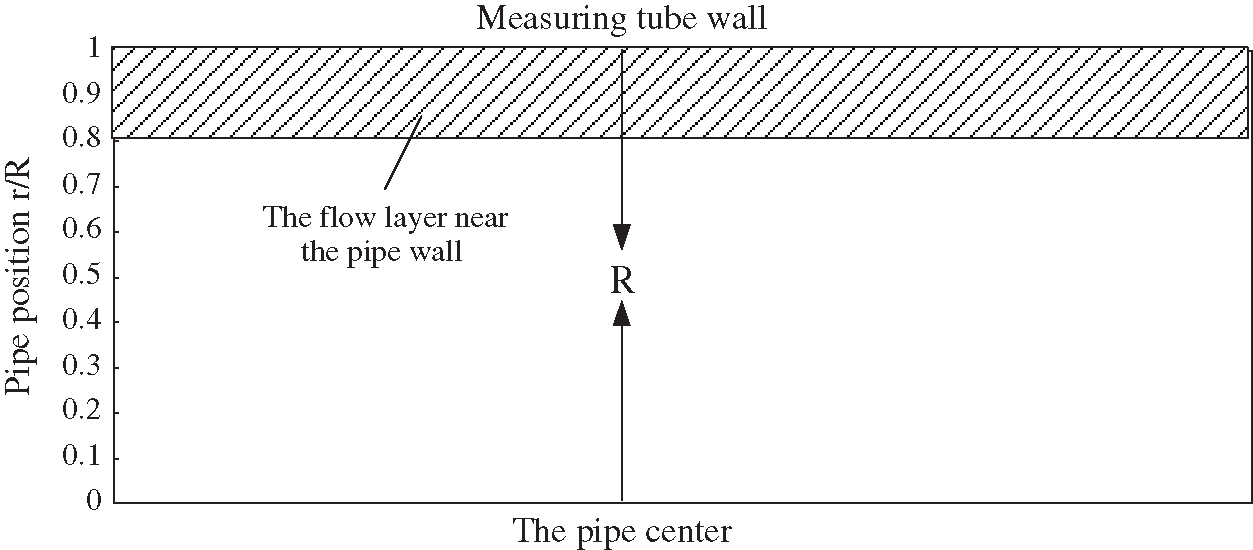
Figure 4: Radial diagram of electromagnetic flow sensor measuring pipe

In the Fig. 4, the distance between any point in the pipe and the center of the pipe is r , R is the pipe radius. The electromagnetic flow sensor measuring pipe is divided into several regions according to the radial direction, and they are determined by r/R , r/R∈[0,1] , r/R=0 indicates the center of the pipe, and r/R=1 indicates the pipe wall. Obviously, according to Fig. 3, the electrode of the electromagnetic flow sensor is installed on the pipe wall, so the electrode is mainly impacted by solid phase particles of fluid near the pipe wall. In this paper, the r/R>0.8 region is taken as the flow layer near the pipe wall, as showed in Fig. 4.

If the average fluid velocity is V¯r/R>0.8 in the r/R>0.8 region, the measured slurry concentration is C¯r/R>0.8 , the solid particle colliding electrode is U1(n) , and U1(n) is a white noise sequence, the amount of particles colliding with electrode in unit time is s , and the variance σ1U2 of U1(n) at this time is assumed to be 1.

After the white noise sequence U1(n) with variance of 1 is taken as the input signal and passes through the 1/f noise filter H(z) , the power spectrum curve of slurry noise signal in coordinate system is obtained:

In Fig. 5, the range of abscissa is 2Hz∼200Hz . The figure shows that, after the white noise sequence U1(n) with variance 1 pass through the filter H(z) , the y-intercept of the power spectral curve is 18 dB, with the increase of frequency, power spectral density curve shows a decreasing trend and has an obvious 1/f characteristic.

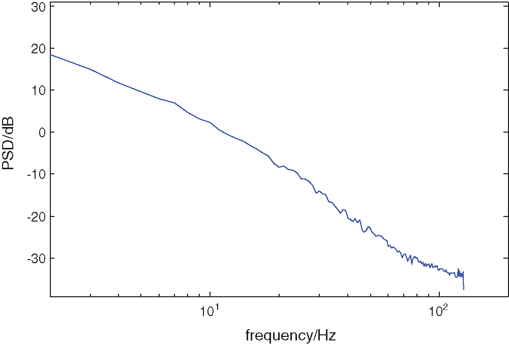
Figure 5: Power spectral density curve of 1/f noise generated by simulation

Because the slurry noise power spectrum of electromagnetic flow sensor has 1/f characteristic, in this paper, this method is used to generate 1/f noise power spectrum to simulate slurry noise of electromagnetic flow sensor.

3  Experimental Verification and Characteristic Analysis of Slurry Noise Power Spectrum of Electromagnetic Flow Sensor

3.1 Slurry Noise Experiment

The diameter is 40 mm electromagnetic flowmeter is experimented, according to experiment, electromagnetic flowmeter measures the range and laboratory equipment, and experiment studies the change situation of slurry noise under different velocity, in the experiment, the slurry fluid with an average volume concentration of 3% in the solid phase is measured when the average flow velocity is 2m/s , 2.8m/s and 3.2m/s in pipe. The experiment is shown in Fig. 6.

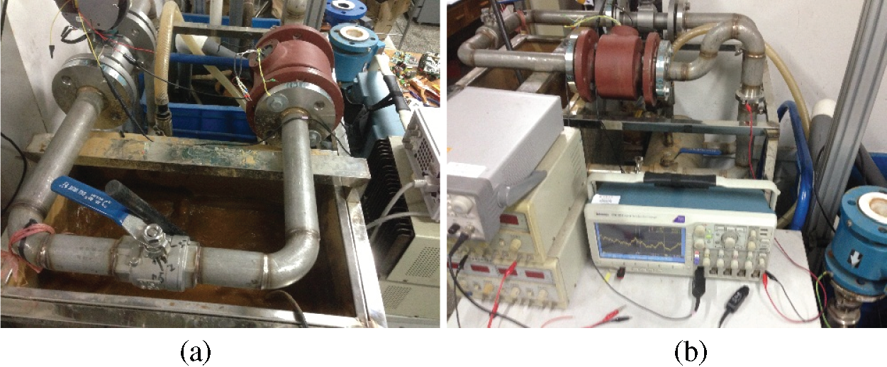
Figure 6: The slurry noise experiment of slurry fluid measured by electromagnetic flowmeter. (a) The slurry fluid experiment; (b) The oscilloscope displays the time domain waveform of slurry noise

In order to observe the time domain waveform of slurry noise on the oscilloscope and collect the slurry noise data, the excitation signal of the electromagnetic flowmeter is switched off during the experiment. It is found in experimenting the frequency range of noise is about 0Hz∼100Hz when the average flow velocity of slurry fluid is 2m/s ~ 3.2m/s , and the intensity amplitude of slurry noise frequency is very smal1 after 100Hz , so the sampling frequency is set as 250Hz . The sampling point is 10000, and the time domain waveform of slurry noise is displayed by oscilloscope, as showed in Figs. 7–9.

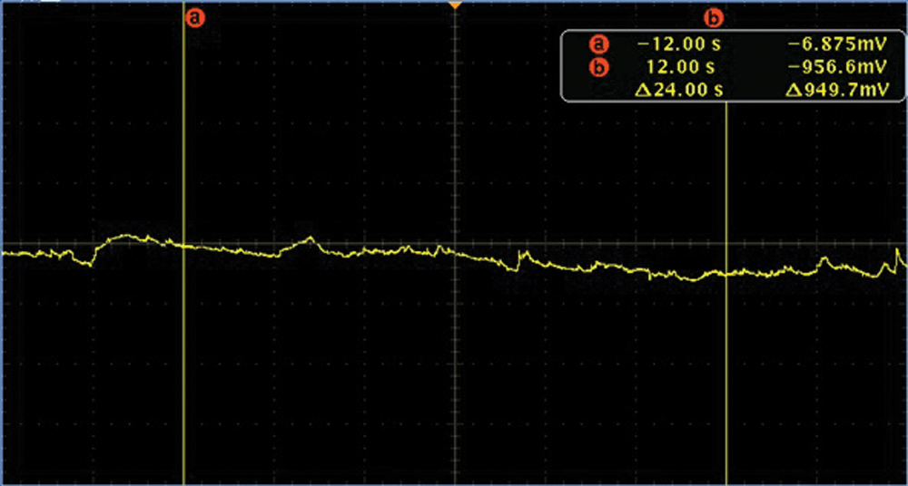
Figure 7: The slurry noise time domain diagram of average flow velocity 2m/s

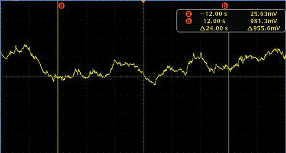
Figure 8: The slurry noise time domain diagram of average flow velocity 2.8m/s

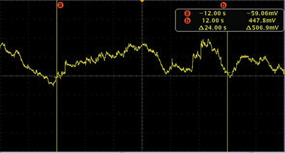
Figure 9: The slurry noise time domain diagram of average flow velocity 3.2m/s

As can be seen from Figs. 7–9, in time domain, the fluctuation amplitude of noise increases with increase of flow velocity, which is caused because of the increasing fluid velocity, the amount of solid phase particles colliding with the electrode of sensor increases in unit time. According to the principle of noise generation, the strength of noise is directly proportional to the total kinetic energy Es of the solid phase particles colliding with electrode in unit time. In this paper, slurry noise intensity is expressed by power P , then:

P∝Es (3)

According to the kinetic energy theorem:

Es=12Ms′sV¯r/R>0.82 (4)

In formula (4), Ms′ is the quality of a single solid particle, and s is the number of solid particles colliding with the measuring electrode. According to formula (3) and formula (4), it is obvious that the intensity of slurry noise is directly proportional to the number of solid phase particles colliding with electrode of electromagnetic flow sensor in unit time, and is directly proportional to the square of the average velocity of flow layer near the pipe wall.

In the situation of the slurry fluid with the initial average volume concentration of 3% in the solid phase is measured when the initial average velocity is 2m/s , 2.8m/s and 3.2m/s in pipe, the total kinetic energy of the solid phase particles colliding with electrode in unit time is Es′3 , Es′4 , Es′5 . If the change of the number s of solid phase particles colliding with electrode and the average flow velocity V¯r/R>0.8 near the measuring electrode can be obtained at the three initial average flow velocity of 2m/s , 2.8m/s and 3.2m/s , the change of total kinetic energy of solid phased particles colliding with electrode in unit time can be obtained after the initial average velocity of the slurry fluid with initial solid phase volume concentration of 3% increased from 2m/s to 2.8m/s and 3.2m/s .

Only consider the two-dimensional situation, average velocity of slurry fluid in the flow layer where the measuring electrode exists is V¯r/R>0.8 . Solid phase particles are groups of particles of different shape and size. Supposing the diameter of particles obey Gaussian distribution, and average diameter is dp . The average volume concentration of solid particles in the flow layer where the measuring electrode exists is C¯r/R>0.8 . The diameter of measuring electrode and fluid contact is de . Only considering the axial movement of the solid particles in the pipe, the number s of solid particles of unit time colliding with the electrode can be calculated by formula (5):

s=V¯r/R>0.8C¯r/R>0.8dedp (5)

According to formula (5), if de and dp can be determined, then the number s of solid phase particles colliding with electrode in unit time is only related to average fluid velocity V¯r/R>0.8 near the pipe wall area and the average volume concentration C¯r/R>0.8 of the liquid solid, namely:

s∝V¯r/R>0.8C¯r/R>0.8 (6)

At present, many scholars use CFD method to study the fluid flow problem, and put forward some new algorithms [40,41]. These documents show that the CFD method is an efficient and reliable method to study slurry flow. Therefore, in the work of this paper, CFD method is used to calculate the above slurry flow parameters.

3.2 Mathematical Model

When the initial average flow velocity is 2m/s , 2.8m/s and 3.2m/s , slurry fluid in the fully developed section of pipe, the average flow velocity V¯r/R>0.8 of the flow layer near the pipe wall.

References [19,20] suggest that Euler-Euler multiphase flow model can be used to simulate and calculate the general problems of multiphase flow. Therefore, in this paper, aiming at the study of sand slurry fluid, Euler-Euler multiphase flow model is used to establish the two-phase flow mechanics model, and RNG turbulence equation [21] is used to describe the turbulent flow of sand slurry fluid.

To establish a mathematical model of sand slurry fluid flow, the following conditions are required:

1.   The solid phase is a continuous fluid, the liquid phase is an incompressible fluid, and the physical properties of each phase are constant.

2.   There is no phase change in both solid and liquid phases, and cavitation phenomenon in the field is not considered.

The equation of motion of slurry fluid is established in Euler coordinate system as follows:

∂ϕL∂t+∂∂xi(ϕLUL)=0 (7)

∂ϕS∂t+∂∂xi(ϕSUS)=0 (8)

where ϕL is the volume fraction of liquid phase, ϕS is the volume fraction of solid phase, UL is the velocity component in the liquid phase, US is the velocity component of the solid phase, and xi is the coordinate component. If the liquid phase density and the solid phase density are ρL and ρS respectively, Eqs. (9) and (10) can be obtained according to Eqs. (7) and (8):

∇(ϕLρLUL)=0 (9)

∇(ϕSρSUS)=0 (10)

Eq. (9) is a liquid phase continuous equation and Eq. (10) is a solid phase continuous equation, the momentum equations are:

∇(ϕLρLULUL)=−ϕL∇p+∇δL+BLS(US−UL)+ϕLρLg (11)

∇(ϕSρSUSUS)=−ϕS∇p−∇pSS+∇δS+BLS(UL−US)+ϕSρSg (12)

where ∇p is the shared pressure of two fluid phases, ∇pSS is the solid pressure caused by the collision of solid particles, δL and δS are the stress tensors of liquid phase and solid phase respectively, g is the gravitational acceleration, and BLS is the momentum transfer coefficient between liquid and solid phases. The value of BLS is related to the volume fraction of liquid phase ϕL , and the detailed calculation method of BLS is given in literature [42]. Only the liquid and solid phases of slurry fluid are considered, therefore:

ϕL+ϕS=1 (13)

then, δL and δS can be determined by Eqs. (14) and (15):

δL=ϕLμL[∇UL+(∇UL)T]−23ϕLμL(∇UL)I (14)

δS=ϕSμS[∇US+(∇US)T]+ϕS(λS−23μS)(∇US)I (15)

where μL is the average effective viscosity of the liquid phase, μS is the solid phase shear viscosity, λS is the solid phase volume viscosity, and I is the unit tensor.

The standard K−ε model was proposed by Launder et al. [43] and is currently the main tool for turbulence calculation in engineering. RNG k−ε model is an improvement on the standard K−ε model and has the following advantages:

a) RNG model adds the additional viscosity term to the N-S equation, and its calculation accuracy is relatively higher.

b) The standard K−ε model can be used for fluids with high Reynolds number, while RNG k−ε model is a lower Reynolds number model.

These characteristics make RNG K−ε model more reliable and accurate than standard k−ε model. Therefore, The RNG K−ε turbulence model is used in this paper.

Using RNG method [44,45] to solve N-S equation and introducing the turbulence kinetic energy k and dissipation rate ε , the following model is obtained:

∇(ρLSULSk)=∇[ak(μ0+μt)∇k]+2μtS2−ρLSε (16)

∇(ρLSULSε)=∇[aε(μ0+μt)∇ε]+2c1εkμtS2−c2ρLSε2k−R (17)

In Eqs. (16) and (17), ρLS is the average density of slurry fluid, ULS is the average speed of slurry fluid, μ0 is the kinematic viscosity of slurry fluid, μt is the turbulent kinematic viscosity coefficient, S=∇ULS , ak , aε , c1 , c2 are constants, according to literature [21], their values are: c1=1.42 , c2=1.68 , ak=aε=1.39 , R is the effect of average strain rate on dissipation rate ε , it is determined by the following equation [21]:

R=cμη3ε2(1−η/ηη0)η0)(1+βη3)k (18)

where η=2Sk/ε , η0 is the typical value of η in uniform shear flow, usually η0=4.38 , the values of other constants are: cμ=0.085 , β=0.012 .

In this paper, the boundary conditions are set as the average velocity inlet and free outflow outlet, the pipe wall is automatically generated by wall function, the pressure is atmospheric pressure, and there is no viscous stress.

3.3 Numerical Calculation

In this paper, we use CFD module of Comsol Multiphysics to carry out the numerical calculation, the calculation method is the finite element method (FEM) [46–49], the calculation is set to the steady state calculation, and the numerical scheme is automatically set by software. The advantage of steady state calculation is that it doesn’t need to obtain the transient value of the flow field, and the steady state results can be used directly, which is helpful to reduce the requirement of computing resources [50]. The work in this paper studies the flow velocity and concentration distribution when the fluid reaches steady state, so the steady state model is suitable.

In order to make sure the grid independence of calculation results, grid testing is necessary. The numerical analysis area is divided into grids, and the number of grids in the calculation area is 17670, 27776, 48588, 73802, 121002, 303530 and 811456, respectively. Under these seven conditions, the velocity and concentration distribution of slurry fluid with initial average velocity V¯ of 2m/s , 2.8m/s , 3.2m/s and initial solid volume concentration C=3% in the fully developed pipe area was calculated. To ensure that the pipe has enough straight length, set the length of the pipe model as 100D , where D is the diameter of the pipe and D=40mm . In order to ensure that the calculation is in the fully developed area of the pipe, the position 50D away from the pipe inlet is selected, and the maximum radial flow velocity Vmax and maximum volume concentration Cmax at this position are shown in Tabs. 1–3.

Table 1: Comparison of the maximum flow velocity and volume concentration for different grid numbers ( V¯=2m/s , C=3% )

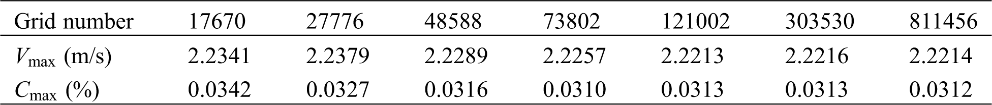
Table 2: Comparison of the maximum flow velocity and volume concentration for different grid numbers ( V¯=2.8m/s , C=3% )

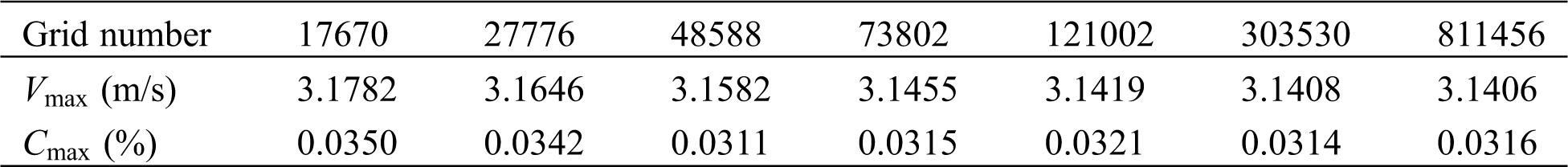
Table 3: Comparison of the maximum flow velocity and volume concentration for different grid numbers ( V¯=3.2m/s , C=3% )

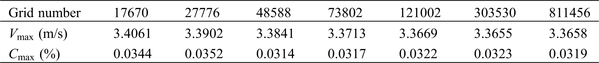
Tabs. 1–3 shows the sensitivity of grids to calculation results, and shows that the number of 303,530 grids is enough to make the solution independent of the number of grids. Therefore, in this paper, the number of calculation area division grids is 303530.

According to CFD method, when the initial average velocity V¯ is 2m/s , 2.8m/s , 3.2m/s , respectively, the initial solid phase volume concentration is C=3% , the nephogram of flow field distribution and concentration distribution is shown in Fig. 10.

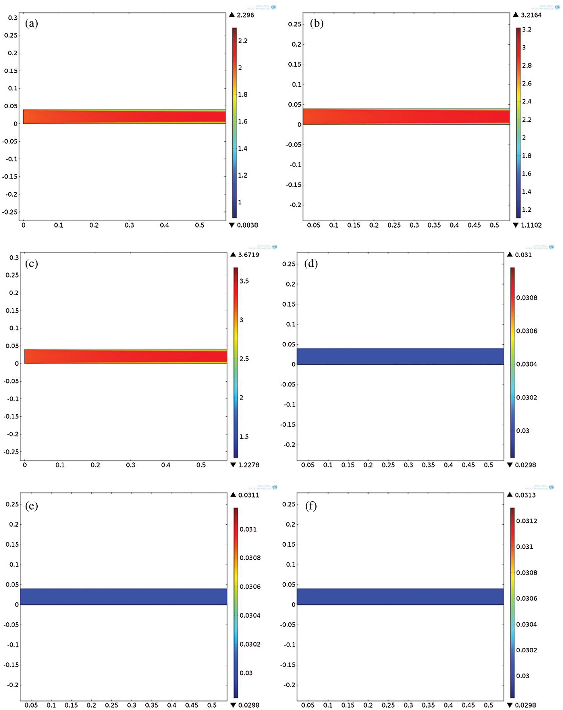
Figure 10: Cloud image of flow field distribution and concentration distribution. (a) Flow velocity distribution ( V¯=2m/s , C=3% ); (b) Flow velocity distribution ( V¯=2.8m/s , C=3% ); (c) Flow velocity distribution ( V¯=3.2m/s , C=3% ); (d) Concentration distribution ( V¯=2m/s , C=3% ); (e) Concentration distribution ( V¯=2.8m/s , C=3% ); (f) Concentration distribution ( V¯=3.2m/s , C=3% )

And the values of V¯r/R>0.8 obtained are:

V1¯r/R>0.8=1.62m/s (19)

V2¯r/R>0.8=2.18m/s (20)

V3¯r/R>0.8=2.49m/s (21)

According to CFD method, it can be calculated that, when the initial average flow velocity is 2m/s , 2.8m/s and 3.2m/s , slurry fluid in fully developed section of pipe, the average solid volume concentration of the flow layer r/R>0.8 near the pipe wall is:

C¯1r/R>0.8=C¯2r/R>0.8=C¯3r/R>0.8=3% (22)

Formula (22) shows that, with the change in flow velocity, the solid phase volume concentration in the flow layer area near the pipe wall remains unchanged.

At the three initial average flow velocity of 2m/s , 2.8m/s and 3.2m/s , the number of solid particles colliding with the electrode in unit time is s1 , s2 , s3 , it can be obtained from formula (19), formula (20), formula (21) and formula (22):

s2s1=V¯2r/R>0.8C¯2r/R>0.8V¯1r/R>0.8C¯1r/R>0.8=1.35 (23)

s3s1=V¯3r/R>0.8C¯3r/R>0.8V¯1r/R>0.8C¯1r/R>0.8=1.54 (24)

according to formula (23) and formula (24), the amount of solid phase particles colliding with electrode increases by 1.35 times and 1.54 times respectively, after the average velocity of slurry fluid with a solid volume concentration of 3% increase from 2m/s to 2.8m/s and 3.2m/s .

The total kinetic energy of solid phase particles colliding with electrode in unit time is Es′1 , Es′2 , Es′3 , when the average velocity of slurry fluid with a solid volume concentration of 3% is 2m/s , 2.8m/s and 3.2m/s , according to formula (4), formula (23), formula (24), formula (19), formula (20) and formula (21), the following formulas can be obtained:

Es′2Es′1=s2V2¯r/R>0.82s1V1¯r/R>0.82=2.46 (25)

Es′3Es′1=s3V3¯r/R>0.82s1V1¯r/R>0.82=3.65 (26)

Formula (25) and formula (26) show that, after the initial average velocity of the slurry fluid with a solid volume concentration of 3% increases from 2m/s to 2.8m/s and 3.2m/s , the total kinetic energy of solid phase particles colliding with electrode increases by 2.46 times and 3.65 times in unit time. According to formula (3), the intensity of slurry noise increases by 2.46 times and 3.65 times, respectively.

3.4 Analysis on Power Spectrum Characteristics of Slurry Noise

In Fig. 11, the x-coordinate ranges from 2 Hz to 200 Hz . As showed in Fig. 11, the power spectral of slurry noise is approximately inversely proportional to the frequency. In the high-frequency part, although the power spectral curve has some fluctuations, on the whole, the curve has a tendency to decline and has an obvious 1/f characteristic. On the basis of the mechanism of slurry noise, frequency of noise is determined by the number of solid particles colliding with electrode at the same time, the high-frequency part is caused by the large number of solid particles colliding with the electrode at the same time, while the low frequency part is caused by the small number of solid particles colliding with electrode at the same time. The number of solid particles colliding with the electrode at the same time is normally distributed in time. Obviously, the amount of particles colliding with the electrode at the same time is inversely proportional to the probability of occurrence. Therefore, the amplitude of the serous noise in the low-frequency part is larger and in the high-frequency part is smaller, the power spectral curve shows the characteristics of 1/f.

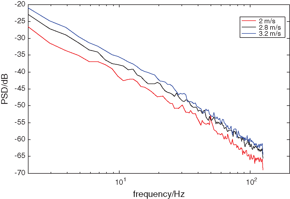
Figure 11: The power spectral of slurry noise

With the increase of average flow velocity, the 1/f characteristic of the power spectral curve of noise remains unchanged, which is manifested as an overall upward shift. Under the condition of average flow velocity is 2m/s , the vertical intercept of the power spectral curve is −27 dB. The average flow velocity increases to 2.8m/s and 3.2m/s , the vertical intercept of the power spectral curve is −23 dB and −21 dB. When the flow rate is 2m/s , 2.8m/s and 3.2m/s , slurry noise intensity of slurry fluid is P1 , P2 , P3 , then:

P2P1=−23dB−(−27dB)=4dB (27)

P3P1=−21dB−(−27dB)=6dB (28)

According to formula (27) and formula (28), formula (29) and formula (30) can be obtained:

P2P1=2.51 (29)

P3P1=3.98 (30)

Formula (29) and formula (30) show that the slurry noise intensity increases by 2.51 times and 3.98 times respectively when the average velocity of slurry fluid with a solid phase volume concentration of 3% increases from 2m/s to 2.8m/s and 3.2m/s , respectively. According to formula (25) and formula (26), the intensity of slurry noise increases by 2.46 times and 3.65 times respectively, it can verify that the theoretical analysis result of slurry noise intensity is basically consistent with the experimental date.

If the solid phase concentration or average velocity of slurry fluid changes, the number s of solid particles colliding with electrode in unit time changes. According to experimental results, it can be known that the power spectral curve of slurry noise will shift in coordinate system. With the power spectral curve obtained by simulation, change the variance σU2 , the change of the amount of solid phase particles colliding with electrode in unit time is equivalent to the shift of power spectral curve. Since the value of s is related to σU2 , it is on1y necessary to determine the solid phase concentration of slurry fluid and the average flow velocity corresponding to variance σU2 , and power spectral of slurry noise generated during the measurement of specific electromagnetic flowmeter can be obtained through simulation.

It can be seen from Fig. 11, the slurry fluid with the solid volume concentration of 3% is measured by the electromagnetic flow sensor with the diameter of 40 mm measures. Under the condition of the average flow velocity of 2m/s , 2.8m/s and 3.2m/s , the vertical intercept of slurry noise power spectral density curve is −27 dB, −23 dB and −21 dB. According to Fig. 5, after H(z) passes the white noise sequence U1(n) with the variance σ1U2 of 1, the vertical intercept of the power spectral curve of simulated noise is 18 dB. The noise intensity is assumed to be Ps , and:

PsP1=18dB−(−27dB)=45dB (31)

PsP2=18dB−(−23dB)=41dB (32)

PsP3=18dB−(−21dB)=39dB (33)

It can be seen from formula (31), formula (32) and formula (33), after H(z) passes the white noise sequence U1(n) with variance σ1U2 of 1, the strength of the 1/f noise of imitated slurry noise is 45 dB, 41 dB and 39 dB higher than the slurry noise generated when the average velocity of slurry fluid is 2m/s , 2.8m/s and 3.2m/s .

According to formula (34):

P=10lg⁡σU2 (34)

So the variance σU2 of the sequence U(n) required by power spectral curve of simulated slurry noise with the average flow velocity of 2 m/s , 2.8 m/s and 3.2 m/s can be calculated. The variance of the white noise sequence is corresponding to the slurry noise with the simulated average velocity of 2 m/s , 2.8 m/s and 3.2 m/s is σ01U2 , σ02U2 and σ03U2 . According to formula (31), formula (32), formula (33) and the formula (34), the following formula can be obtained:

10lgσ1U2σ01U2=45dB (35)

10lgσ1U2σ02U2=41dB (36)

10lgσ1U2σ03U2=39dB (37)

As σ1U2=1 , the values of σ01U2 , σ02U2 and σ03U2 is 3.2×10−5 , 7.9×10−5 and 1.26×10−4 . So the power spectral curve with simulated average velocity of 2m/s , 2.8m/s and 3.2m/s can be simulated, as showed in Fig. 12.

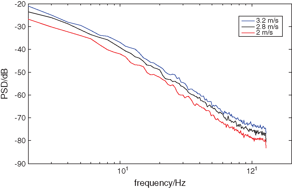
Figure 12: The power spectrum of slurry noise obtained by simulation

It can be seen from Fig. 12, according to formula (35), formula (36) and formula (37), after σ01U2 , σ02U2 and σ03U2 is obtained, the position of the power spectrum curve of the simulated slurry noise approximately equals with the power spectrum curve of the simulated slurry noise obtained from the experiment as shown in Fig. 11 in the coordinate system, thus the correctness of the simulation method and simulation results is verified. Simulation results show that:

1.   With the change of average flow velocity, the amount of solid phase particles colliding with electrode changes from unit time, the variance of the corresponding white noise sequence changes, and the position of power spectral curve of simulated slurry noise also changes in coordinate system.

2.   If the amount of solid phase particles colliding with electrode increases in unit time, the variance of the corresponding white noise sequence increases, and the power spectrum curve of the slurry noise shifts upward. If the number of solid phase particles colliding with electrode decreases in unit time, the variance of the corresponding white noise sequence decreases, and the power spectrum curve of slurry noise shifts downward.

3.   The power spectrum curve of slurry noise reflects the intensity of slurry noise, the upward translation of the curve indicates that the intensity of slurry noise increases, the downward translation of the curve indicates that the intensity of slurry noise decreases.

4  Conclusion

In this paper, firstly, on the basis of the 1/f characteristic of the power spectrum of slurry noise, based on Matlab software, the slurry noise is simulated by using the 1/f noise filter passed by Gaussian white noise. Then, the relationship between intensity of slurry noise and the amount of solid phase particles impacting the electrode of electromagnetic flow sensor in unit time and the average flow velocity of the flow layer near the pipe wall is analyzed through slurry experiments, and the simulation of slurry noise is verified. Finally, according to the slurry noise power spectrum curves under different flow velocities obtained from the slurry fluid experiments and simulations, the variation law of the slurry noise power spectrum curve with the flow velocity is obtained, and the conclusions are as follows:

1.   On the basis of the cause of slurry noise and 1/f characteristic of power spectrum, slurry noise power spectrum can be generated by Matlab simulation, and the real slurry noise power spectrum can be simulated as long as the variance of Gaussian white noise is adjusted as required.

2.   The intensity of slurry noise is directly proportional to the amount of solid phase particles impacting electrode in unit time and square of the average velocity of flow layer near the pipe wall.

3.   With the change of average flow velocity of measured fluid, the position of power spectral curve of slurry noise changes in coordinate system. Specifically, if the average velocity increases, the power spectral curve of slurry noise will shift upward, and if the average velocity decreases, the power spectral curve will shift downward.

The above conclusions can improve the related theory of electromagnetic flow sensor in slurry measurement field to a certain extent, and provide a certain theoretical basis of the research and development of electromagnetic flow sensors for slurry fluid flow measurement.

The deficiency of this paper is that due to the limitation of experimental conditions, there is still a lack of using mechanical models to prove the conclusion and give physical insight. Therefore, the work of this paper is worthy of further study in verifying the conclusion by using the mechanical model. In addition, in the future research, we will consider using CFD method to verify the experimental results in this paper.

Funding Statement: This work was sponsored by National Key Research and Development Program of China Subproject (No. 2016YFD0700103), Natural Science Foundation of Henan (Nos. 202300410124 & 19HASTIT021), Key Research and Development Program of Yunnan Province (No. 2018ZC001) and the National Natural Science foundation of China under Grant No. 61801288.

Conflicts of Interest: The authors declare that they have no conflicts of interest to report regarding the present study.

This work is licensed under a Creative Commons Attribution 4.0 International License, which permits unrestricted use, distribution, and reproduction in any medium, provided the original work is properly cited.