Fluid Dynamics & Materials Processing

DOI: 10.32604/fdmp.2021.011914

ARTICLE

Flow Simulation of a Horizontal Well with Two Types of Completions in the Frame of a Wellbore–Annulus–Reservoir Model

Qinghua Wang1, Junzheng Yang1 and Wei Luo2,*

1PetroChina Research Institute of Petroleum Exploration & Development, Beijing, 100083, China
2Petroleum Engineering Institute of Yangtze University, Wuhan, 430100, China
*Corresponding Author: Wei Luo. Email: luowei16@yangtzeu.edu.cn
Received: 05 July 2020; Accepted: 24 December 2019

Nomenclature

:	the intermediate substitution variable
:	the volume factor of crude oil
:	the intermediate substitution variable
:	integral constant of segment j
:	integral constant
:	the intermediate substitution variable
:	the internal diameter of the casings [m]
:	the equivalent diameter of the annulus (i.e., area equivalent) [m]
:	the diameter of the center tubing [m]
:	the loss of annular pressure drop of the i infinitesimal section of the annulus pipe flow [Pa]
:	the loss of pressure drop of the i infinitesimal section of the center cylindrical pipe flow [Pa]
:	the friction loss in the i infinitesimal section of the center tubing [Pa]
:	the acceleration loss in the i infinitesimal section of the center tubing [Pa]
:	the mixing loss in the i infinitesimal section of the center tubing [Pa]
:	the friction loss in the i infinitesimal section of the annulus [Pa]
:	the acceleration loss in the i infinitesimal section of the annulus [Pa]
:	the mixed pressure drop loss of the annular area of the i infinitesimal section [Pa]
:	the full differential of (or the length of the i infinitesimal section that is equal to ) [m]
:	the differential of the independent variable x [m]
:	the differential of the independent variable y [m]
:	the differential of the independent variable z [m]
:	the frictional factor of the i infinitesimal section
:	the friction factor of the annular area of the i infinitesimal section
:	the intermediate substitution function
:	the intermediate substitution function
:	the acceleration of gravity [m/s2]
:	the intermediate substitution function
:	the height difference from the reservoir bottom [m]
:	the thickness of the oil layer [m]
:	the horizontal permeability [m2]
:	the vertical permeability [m2]
:	the permeability [m2]
:	the length of segment j [m]
:	the length of horizontal well [m]
:	the num of divided segments of horizontal well (a uniform flow section)
N:	the num of divided segments of horizontal well (which consists of many non-uniform flow segments)
:	the upstream pressure of the i infinitesimal section of the annulus pipe flow [Pa]
:	the downstream pressure of the i infinitesimal section of the annulus pipe flow [Pa]
:	the upstream pressure of the i infinitesimal section of the center cylindrical pipe flow [Pa]
:	the downstream pressure of the i infinitesimal section of the center cylindrical pipe flow [Pa]
:	the formation pressure of the drain boundary [Pa]
:	the flow pressure in the center cylinder of the i infinitesimal section [Pa]
:	the pressure in the annulus of the i infinitesimal section [Pa]
:	the bottom hole flow pressure [Pa]
:	the pressure in the oil layer [Pa]
:	the upstream flow rate of the i infinitesimal section of the center cylindrical pipe flow [m3/s]
:	the downstream flow rate of the i infinitesimal section of the center cylindrical pipe flow [m3/s]
:	the production rate of horizontal well [m3/s]
:	the upstream flow rate (it may also be negative, which indicates a reverse flow) of the i infinitesimal section of the annulus pipe flow [m3/s]
:	the downstream flow rate of the i infinitesimal section of the annulus pipe flow [m3/s]
:	the flow rate of the i infinitesimal section from the oil layer into the annulus [Pa]
:	production rate [m3/s]
:	the flow radius [m]
:	the distance (approximate length) from the start point of the ith segment to the final point (, , ) obtained in this segment [m]
:	the mainstream velocity at the beginning of the i infinitesimal section of the center tubing [m/s]
:	the mainstream velocity at the end of the i infinitesimal section of the center tubing [m/s]
:	the velocity of the i infinitesimal section from the annulus into the center tubing [m/s]
:	the mainstream velocity at the beginning of the i infinitesimal section of the annulus [m/s]
:	the mainstream velocity at the end of the i infinitesimal section of the annulus [m/s]
:	the velocity of the i infinitesimal section flowing from the formation into the annulus [m/s]
:	the Darcy velocity [m/s]
:	the x coordinate of any point in space [m]
:	the start x coordinate of (the 1th segment of) segment j [m]
:	the end x coordinate of (the mth segment of) segment j [m]
:	the x coordinate of the start point of the ith segment of horizontal well [m]
:	the x coordinate of the end point of the ith segment of horizontal well [m]
:	the x coordinate of the start point of horizontal well [m]
:	the x coordinate of the end point of horizontal well [m]
:	the y coordinate of any point in space [m]
:	the start y coordinate of the ith segment of segment j [m]
:	the end y coordinate of the ith segment of segment j [m]
:	the y coordinate of the end point of the ith segment of horizontal well [m]
:	the y coordinate of the start point of the ith segment of horizontal well [m]
:	the y coordinate of the start point of horizontal well [m]
:	the y coordinate of the end point of horizontal well [m]
:	the z coordinate of any point in space [m]
:	the distance from the horizontal well to the bottom of the layer [m]
:	the start z coordinate of the ith segment of segment j [m]
:	the end z coordinate of the ith segment of segment j [m]
:	the z coordinate of the start point of the ith segment of horizontal well [m]
:	the z coordinate of the end point of the ith segment of horizontal well [m]
:	the z coordinate of the start point of horizontal well [m]
:	the z coordinate of the end point of horizontal well [m]
:	the height of the drain boundary [m]
:	the height of the well in the reservoir [m]

Greek letters

:	The potential produced by well production
:	Viscosity [Pa.s]
:	The intermediate substitution function (equals to the formula within the outer layer braces of the Formula (23))
:	the potential of the constant pressure boundary or the oil drainage boundary
:	the potential generated by the segment j at the constant pressure boundary or the oil drainage boundary
:	the density of the fluid [kg/m3]
:	the potential generated by the i segment line at the midpoint of the j segment line
:	the micro-velocity variation in the micro-distance variation from the formation into the annulus [m/s]
:	the micro-velocity variation in the micro-distance variation from the annulus into the center tubing [m/s]
:	the micro-distance variation from the beginning of the i infinitesimal section of the center tubing [m]
:	The intermediate substitution function
:	the inclination angle from the horizontal plane of the i infinitesimal section [°]
:	the flow rate of the i infinitesimal section from the annulus into the center tubing [Pa]
:	the additional pressure drop between tubing and annulus at the beginning of the i infinitesimal section under different completion modes [Pa]
:	the additional pressure drop between tubing and annulus at the end of the i infinitesimal section under different completion modes [Pa]
:	The segment length [m]

Subscript

:	annulus wellbore
:	wellbore
:	the i infinitesimal section (segment)
:	the friction loss of the center tubing
:	the acceleration loss of the center tubing
:	the mixing loss of the center tubing
:	the mixing loss of the annulus (middle)
:	the acceleration loss of the annulus (middle)
:	the mixed pressure drop loss of the annulus (middle)
:	horizontal
:	vertical
:	the infinitesimal section (segment)
:	the start of one segment of annulus
:	the end of one segment of annulus
:	the start of one segment of tubing
:	the end of one segment of tubing
:	the initial condition of the drain boundary
:	the bottom hole wellbore flow
:	sum of
:	tubing radial direction
:	casing radial direction
:	the start of the ith segment of segment j
:	the end of the ith segment of segment j

1  Introduction

Accurately predicting the productivity of horizontal wells is crucial to the formulation of horizontal well production system and parameter optimization. Establishing an accurate horizontal well productivity prediction model [1] or production data analysis model [2] is a work we have been doing. Slotted screen completions and inflow control device (ICD) completions are two of the most common completions used in horizontal well completion methods. Fluid flows from the oil reservoir into the wellbore through these completions, which results in an additional pressure drop affecting the production rate of horizontal wells. However, prediction models for horizontal well production rates based on slotted screen and ICD completions have been simplified so that only the flow in the center tubing is considered, while the flow in the annulus is disregarded [3–8]. Valvatne et al. [9] and Neylon et al. [10] established corresponding models for ICD completions, but did not consider the effects of annulus flow. Luo et al. [11,12] presented a more detailed model for ICD completions than the previous models but did not clearly analyze how annulus flow affects the production rate through the flow rate profile and pressure drop profile along the center tubing and the annular wellbore. The flow in horizontal wells from the wellbore–annulus–reservoir processes of slotted screen completions and ICD completions has not been considered. The physical process of fluid flow in slotted screen completions and ICD completions is shown in Fig. 1. There are actually two types of variable mass flow in the horizontal wellbore: central tubing flow and annulus flow. These two flow factors are important. Lorenz et al. [13] conducted production simulations with and without an ICD within an 8.53 m horizontal wellbore and compared the annular flow under the two conditions. Their experiments showed that during actual production, if the flow profile of the horizontal section is unevenly produced, the horizontal section of the slotted screen completion and ICD completion will contain the variable mass flows of the center tubing and the annulus, as shown in Fig. 2.

Figure 1: Actual physical simplified model of a screen completion

Figure 2: Diagram of horizontal well flow

In this work, the authors have considered the wellbore-annulus-reservoir process in the horizontal section of a slotted screen completion and ICD completion. A corresponding flow model, a reservoir Darcy flow, and a prediction model for the production rate of horizontal wells is proposed. Furthermore, the developed model is compared with existing models with and without annulus flow modeling.

2  Establishment of Coupled Mathematical Model

Horizontal well production involves two flow processes: The flow of fluid in the formation section and the flow of fluid in the wellbore section. In this study, models for fluid flow in the reservoir and in the wellbore are developed. The two models are then coupled to establish a prediction model for the production rate of horizontal wells.

2.1 A 3D Steady Darcy Flow Model that Considers the Real Wellbore Trajectory

A 3D steady Darcy flow model that considers the real wellbore trajectory in this paper uses the model in Luo et al. [14].

2.2 Fluid Flow Model in the Wellbore Section

(1) Computation model for the flow rate and flow pressure of the infinitesimal section

The length of the wellbore section is represented as L and is divided into N segments. The segment length is when sorting is conducted from toe to heel. The diagram of infinitesimal section i is provided in Fig. 3. In the infinitesimal section i of the center cylindrical pipe flow, denotes the upstream pressure, denotes the upstream flow rate, denotes the downstream pressure, denotes the downstream flow rate, and denotes the loss of pressure drop in the segment.

In the infinitesimal section i of the annulus pipe flow, represents the upstream pressure, represents the upstream flow rate (which may also be negative, which indicating a reverse flow), represents the downstream pressure, represents the downstream flow rate, and represents the loss of annular pressure drop in the segment.

The following relationships are then derived:

In the preceding formulas, indicates the flow rate of infinitesimal section i from the annulus into the center tubing, indicates the flow rate of infinitesimal section i from the oil layer into the annulus, indicates the additional pressure drop between the tubing and annulus at the beginning of infinitesimal section i under different completion modes, and indicates the additional pressure drop between the tubing and annulus at the end of infinitesimal section i under different completion modes. For the slotted screen completion, details are provided in Xiong et al. [15]. The ICD completion uses a spiral channel-type ICD [16].

Figure 3: Flow diagram and force analysis of infinitesimal section i

The flow pressure in the center cylinder of infinitesimal section i considers the average value of pressure in the following section:

The flow pressure in the annulus of infinitesimal section i considers the average value of the following section pressure:

Assuming that no initial flow is observed at the toe of the wellbore, . Thus, the flow pressure at the end of the horizontal section is equal to the bottom hole flow pressure . Accordingly, the following equation is applied:

(2) Calculation model for pressure–loss in infinitesimal section i

The pressure loss in the center cylinder of infinitesimal section i includes the gravity loss, friction loss, acceleration loss, and mixing loss. Assume that is the friction loss in infinitesimal section i (Pa), is the acceleration loss (Pa), and is the mixing loss (Pa). The value of the mixing loss is zero (0) in this study. In accordance with the principle of conservation of mass [17]:

The following equation can be derived:

where is the density of the fluid (kg/m3), D is the diameter of the center tubing (m), is the mainstream velocity from the beginning of infinitesimal section i to the center tubing (m/s), is the velocity of infinitesimal section i from the annulus into the center tubing (m/s), is the microvelocity variation in the microdistance variation from the annulus into the center tubing (m/s), and is the microdistance variation from the beginning of infinitesimal section i to the center tubing (m).

The annular pressure loss in infinitesimal section i includes the gravity loss, friction loss, acceleration loss, and mixing loss. Assume that is the friction loss in infinitesimal section i (Pa), is the acceleration loss (Pa), and is the mixing loss (Pa). In accordance with the principle of conservation of mass:

When the preceding equation is combined with the mass conservation formulas of the center tubing, we obtain

where is the mainstream velocity from the beginning of infinitesimal section i to the annulus (m/s), is the velocity of infinitesimal section i flowing from the formation into the annulus (m/s), is the internal diameter of the casings (m), and is the microvelocity variation in the microdistance variation from the formation into the annulus (m/s).

As shown in Fig. 3 and based on the principle of momentum conservation, the calculation of total pressure loss in the center is

where is the acceleration due to gravity (m/s2), is the inclination angle from the horizontal plane of infinitesimal section i (°), is the frictional factor, is the mainstream velocity from the end of infinitesimal section i to the center tubing, and is the length of infinitesimal section i that is equal to (m).

In accordance with the principle of momentum conservation, the calculation of total annular pressure loss is obtained as

In the preceding formulas, denotes the annulus pressure drop in infinitesimal section i (Pa), denotes the equivalent diameter of the annulus (i.e., area equivalent) (m), denotes the friction factor of the annular area, is the mainstream velocity from the end of infinitesimal section i to the annulus (m/s), and is the mixed pressure drop loss (Pa). The values of the mixed pressure drop in this study are 0.

2.3 Steady-State Coupling and Its Solution

Assume that is the pressure at the midpoint of the center of section j for the horizontal well. The pressure at the midpoint of the annulus in section j is

Assuming that is the potential generated by segment line i at the midpoint of segment line j, integrating Eq. (8) [14] yields

where is the formation pressure of the drain boundary (Pa), is the fluid viscosity (Pa.s), is the permeability (m2), is the height of the drain boundary (m), and is the height of the well in the reservoir (m).

The preceding formula is then rearranged as follows and is similar to Formula (20) [14]

where .

The pressure drop in the center tubing can be calculated using Eq. (20). The pressure at the midpoint of section j for the center tubing is

From Eq. (21), , and is the heel end pressure of the wellbore.

The total well output is

where is the volume factor of crude oil and is the production rate of the horizontal well.

In the coupled model, and are unknown, but can be determined by using an iterative method. Suppose that a group of values and solutions with Eq. (20) is available to obtain the numerical value of q. Then, q is substituted into pressure drop Eqs. (7), (8), (16), (18), and (21). is updated from the heel to the toe, and the value of q is updated using Eq. (20). These procedures are repeated until and q reach the desired accuracy. Finally, Eq. (23) is used to obtain the output for the whole well. The specific calculation flow chart is shown in Fig. 4 below.

Figure 4: The calculation flow chart

3  Case Calculation and Comparison with CMG Simulation Software

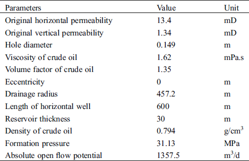
Well No. XXX-1 in the reservoir of the Halfaya Oilfield with bottom water in Iraq is selected as an example, as shown in Tab. 1. The slotted screen completion and ICD completion are simulated using the model established in this study and the simulation software from the Computer Modeling Group, Ltd., (Alberta, Canada) with and without considering the simulation of annulus flow conditions.

Table 1: Basic data for Well XXX-1

3.1 Calculation and Comparison of the Example with Slotted Screen Completion with and without Considering Annulus Flow

The parameters of the slotted screen completion are as follows: The outside diameter of the screen is 114.3 mm with 120 holes per meter. The hole diameter is 10 mm, and holes are uniformly distributed. A thin filter sleeve layer is placed outside the screen. The well test showed that the screen has an evident sand layer. The permeability of the sand layer is 14,000 mD based on the absolute open flow potential of the oil well. It is assumed that no packer is placed outside the screen and that the bottom hole pressure is 0 MPa in the heel. Horizontal well pressure profiles and liquid production profiles (the point of the production rate is the total rate at 10 m) are shown in Figs. 5 and 6, with and without considering annulus flow. The total output and the absolute relative error are shown in Tab. 2.

The information presented in the graphs (Figs. 5 and 6) and Tab. 2 show that the prediction of the model without annulus flow modeling is 9.51% higher than that of the model with annulus flow modeling and that the pressure values of the borehole wall and the flow profile are more uniform in the model with annulus flow modeling. The error between the two flow models can be reduced if an appropriate number of packers is placed outside the pipe. The results of the flow profile of the center tubing calculated using the model with annulus flow modeling clearly show a flow in the annulus from the toe to the heel to aggregate flow into the center tubing.

Table 2: Production predicted by the two models

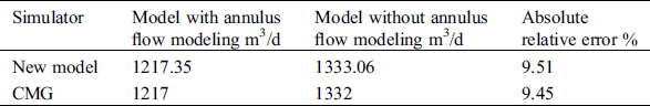
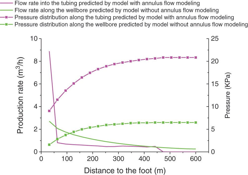
Figure 5: Profiles of pressure distribution and flow into the tubing (or along the wellbore) are calculated using the two flow models for the slotted screen

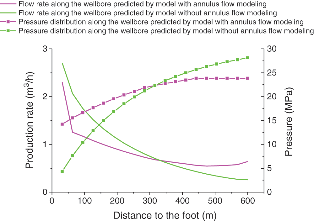
Figure 6: Profiles of pressure distribution and flow along the borehole are calculated using the two flow models for the slotted screen

CMG is a three-phase black oil simulation software that considers gravity and capillary force. The network system can use rectangular coordinates, radial coordinates, and variable depth/variable thickness coordinates. In any network system, two or three-dimensional models can be established. This model selected is the Implicit-explicit Black Oil Simulator (IMEX) in the CMG software, which is an adaptive implicit black oil simulation software (adaptive implicit numerical simulation method) for simulating gas and gas- Three-phase flow of water, oil-water, and oil-gas-water reservoir fluids. IMEX can run in three modes: display, full implicit and adaptive implicit. In most cases, only a small part of the mesh needs to be solved fully implicitly, and most of the grids can be solved by explicit methods. The adaptive implicit method is just the solution method suitable for this situation, and in the well Nearby and in the thin layers of layered oil reservoirs, high-speed flow coning problems will occur during production. It is very effective to adopt adaptive implicit processing to deal with these problems. Using adaptive implicit options can save one-third to half of the running time. The calculation can use the same large time step as the full implicit method. The user can specify the grid to be calculated by the full implicit method, and the network that uses the full implicit calculation can be dynamically selected according to the user-defined limit or matrix conversion critical value grid.

On the basis of the reservoir, fluid, and oil well parameters, simulation mechanism models for wellbore flow with and without annulus flow are established using the CMG FlexWell function. The screen hole flow of the screen completion is simulated using the ICD Orifice model because their flows are similar. The grid size is 92 × 92 × 3 m3, and each grid is 10 m. The horizontal well is located in the middle level of the grid, and its length is 600 m. In addition, the values of other parameters (such as the diameter of the well) are the same as the values of the corresponding parameters in the example. The open hole place of the pipe string is located in the middle of each grid, and thus, the distance between the front and rear holes is 580 m. The hole size and the number of ICD orifices are the same as those in screen completion. The model is shown in Figs. 7 and 8.

This model first uses IMEX to build a reservoir model, and inputs rock physical properties and fluid properties (oil-gas-water PVT data and rock PVT properties, oil-gas permeability curves, etc.) to complete the reservoir model. Then use CMG’s FlexWell to build an ICD (or screen) completion horizontal well production model. FlexWell can simulate the production of complex oil wells by establishing the oil well model shown in Figs. 9 and 10 below. Among them, the annulus is bound to the prdan well to simulate the annulus, and the tubing is bound to prdtb to simulate the tubing. In this way, the operation of establishing the real flow model of horizontal well ICD completion (considering the annulus flow) through CMG software is realized.

The CMG FlexWell can achieve the simultaneous production of the annulus and tubing by setting the outer and inner pipes. In view of this feature, this article uses the setting of the outer and inner pipes to simulate the simultaneous flow of the annulus and central tubing. The annulus flow finally enters the tubing, so this paper sets up a packer at the heel end so that the annulus heel end cannot flow upwards to achieve the simulation situation required in this article.

Fig. 11 presents the simulation results of different CMG models when the production is stable. However, the CMG models do not provide the pressure distribution and flow profile along the borehole. The figure also shows that the simulation results (profiles of pressure and production) of the flow model without annulus flow are consistent with the simulation results of the corresponding model in Fig. 5 when the well production rate is 1332 m3/d, which is the same as the production rate of the model established in this study (Tab. 2). The simulation results (well production is shown in Tab. 2) for the wellbore flow model with annular flow are also consistent with the simulation results of the corresponding model in Fig. 5. The CMG simulator can simulate the flow from the annulus into the tubing. The flow rule along the center tubing in the simulation results can reflect the authenticity of the simulation results of the established model from the annulus wellbore, which is also consistent with the results of this study.

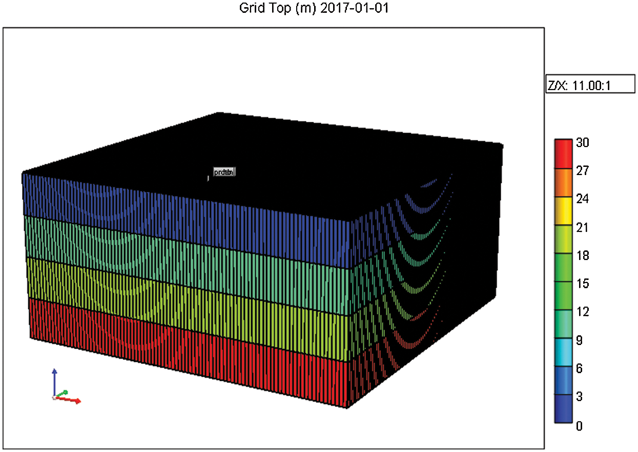
Figure 7: Stereoscopic grid model

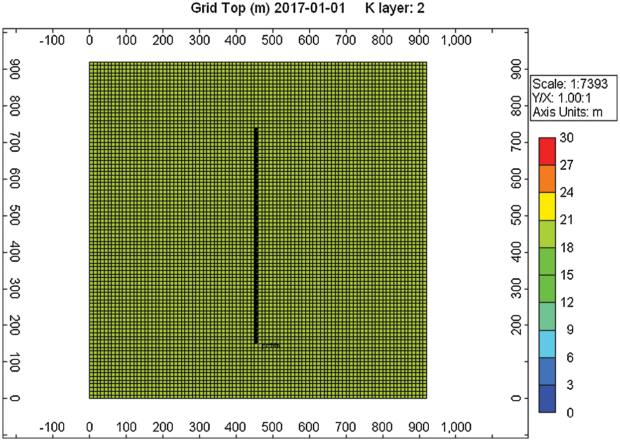
Figure 8: Plane grid model of the well and middle horizons

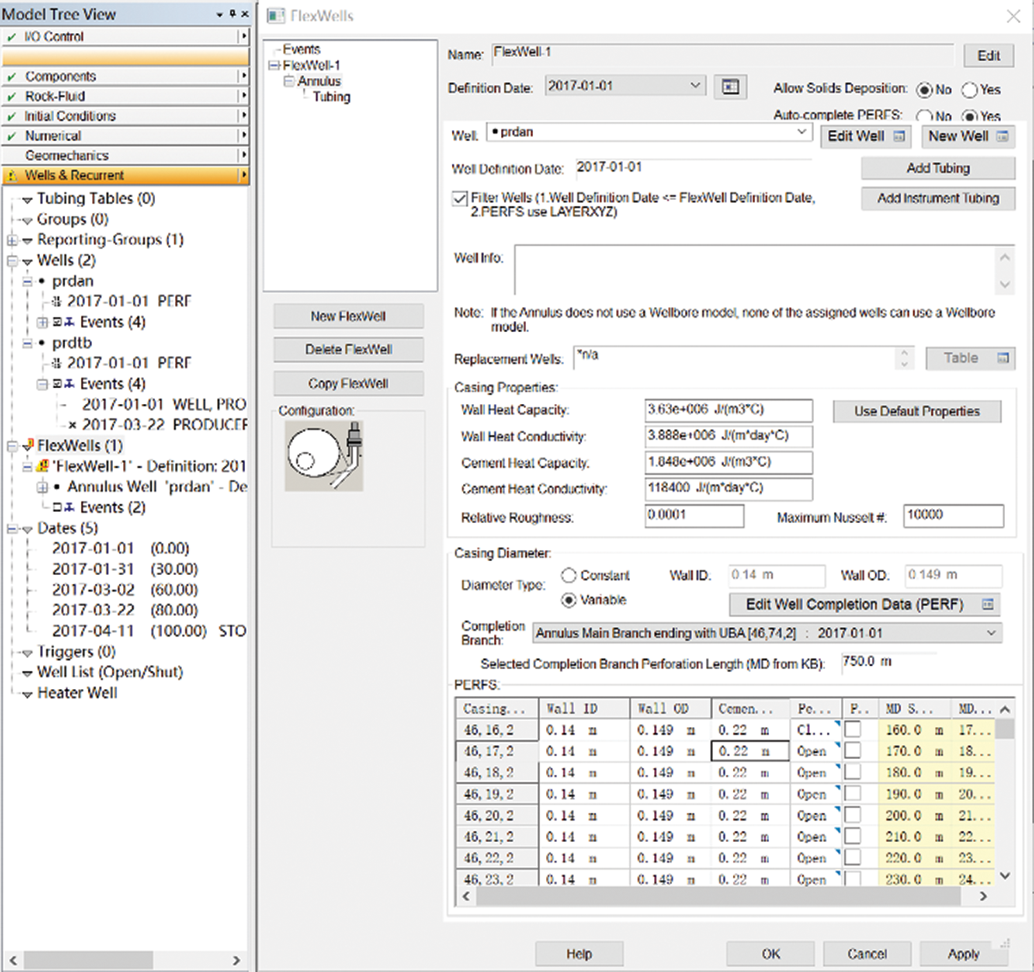
Figure 9: Production configuration of annulus passage between tubing and casing

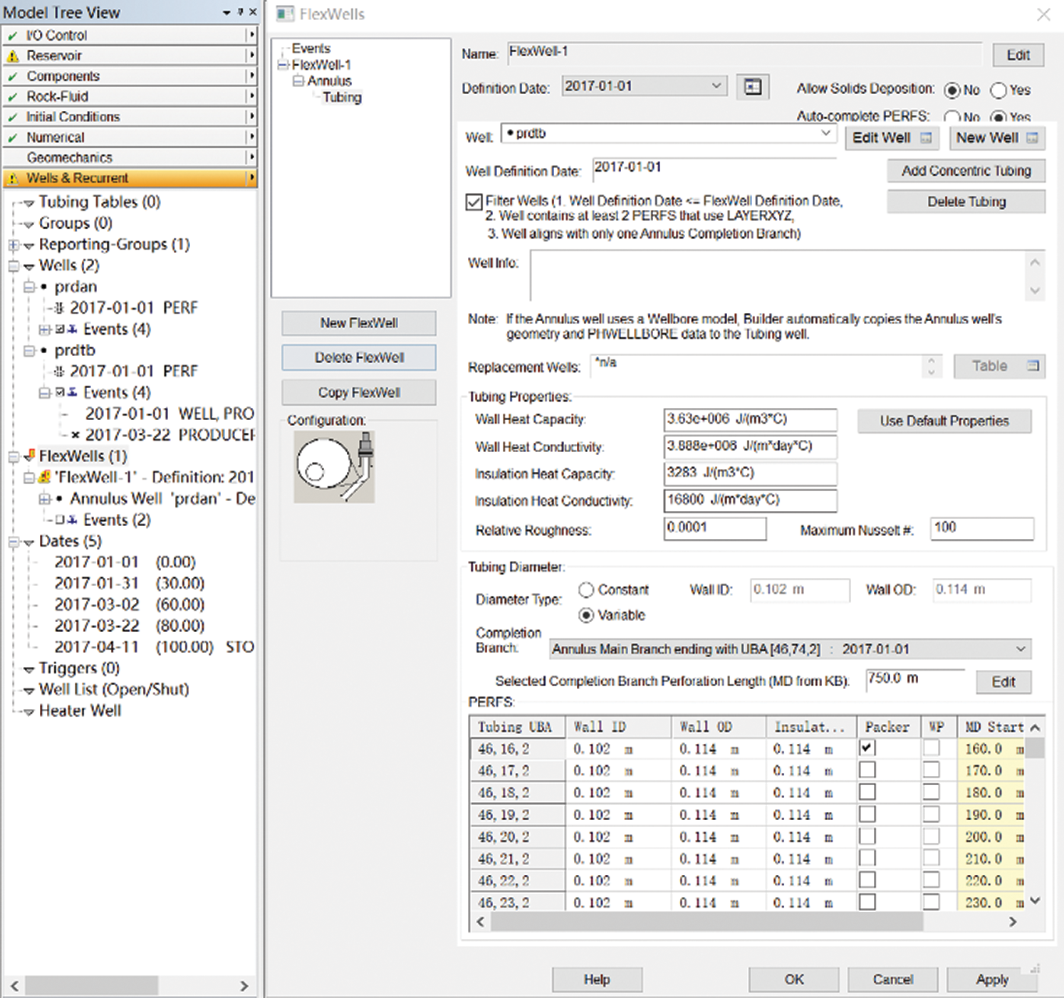
Figure 10: Central tubing configuration

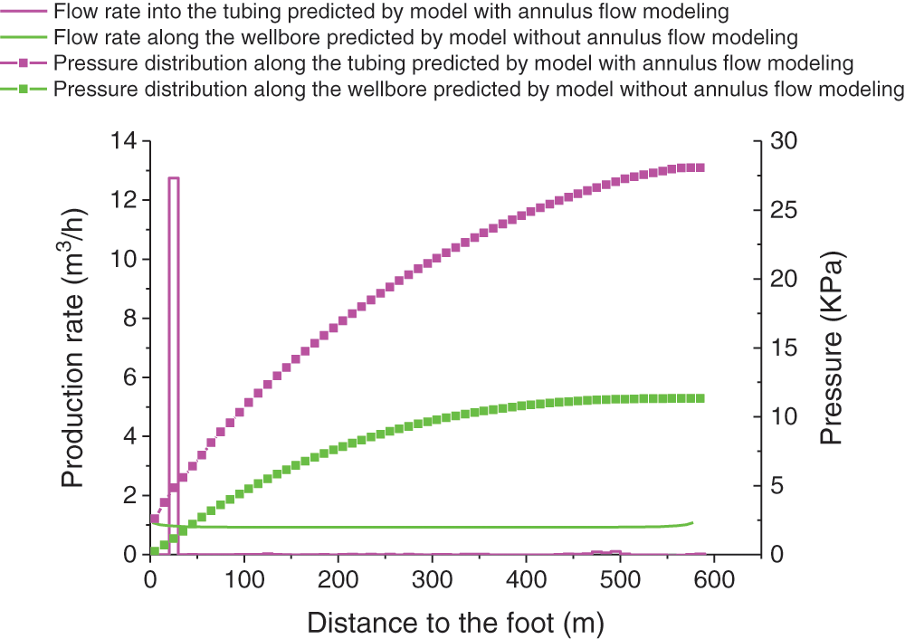
Figure 11: Profiles of pressure distribution and flow into the tubing (or along the wellbore) are calculated using the two flow models for the slotted screen in the CMG simulator

3.2 Calculation and Comparison of the Example with ICD Completion with and without Considering Annulus Flow

Assuming that the well is completed with an ICD, and that no sand has accumulated outside the pipe, the ICD completion parameters are as follows: the outside diameter of the ICD completion is 114.3 mm, the length (throttling device) of a single throttle tube is 2 m, the diameter of the throttle tube is 3 mm, and the local head loss factor is 0.16. Furthermore, assuming that the entire horizontal section of the ICD is arranged, the ICD pipe has no packer, and the bottom hole pressure is 0 MPa in the heel. The horizontal well pressure profiles and liquid production profiles are shown in Figs. 12 and 13, with and without considering the annulus flow. The total output and the absolute relative error are presented in Tab. 3.

The information presented in the graphs (Figs. 12 and 13) and Tab. 3 show that in the prediction of ICD well completion, the result of the model without annulus flow modeling is 70.98% higher than that of the model with annulus flow modeling. Moreover, the pressure and flow profiles along the borehole wall are more uniform. Although the calculation example assumes that no packer is placed outside the tube and the absolute relative error of the predicted production between the two models is considerable, the real completion pipe with a certain number of packers reduces only the error between the models with and without annulus flow modeling prediction results. When the out-of-pipe packer condition is considered, the error between the models with and without annulus flow modeling can still be significant. The specific error is related to the number and positions of packers outside the pipe, and further research can be conducted based on the model with annulus flow modeling. The results of the flow profile of the center tubing calculated using the ICD model with annulus flow modeling also show a clear flow in the annulus from the toe to the heel to aggregate flow into the center tubing.

Table 3: Production predicted by the two models

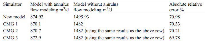
Figure 12: Profiles of pressure distribution and flow into the tubing (or along the wellbore) are calculated using the two flow models for the ICD

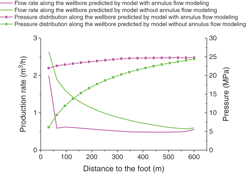
Figure 13: Profiles of pressure distribution and flow along the borehole are calculated using the flow models for the ICD

Similarly, the mechanism models with and without annular flow are established via the CMG FlexWell function according to the parameters of the reservoir, fluid, and oil well. The ICD orifice model is also used to simulate the ICD friction pressure drop. The ICD friction pressure drop model is also adopted in the CMG simulation. Despite the easy flow conditions, the simulation produces no results for production. Therefore, only the ICD orifice model can be used for the simulation. The hole size and number of ICD orifices are the same as those in ICD friction. Pressure drop-type completion (throttling device) and the flow that corresponds to the flow of ICD friction pressure drop-type completion can be adjusted by setting the diffusion coefficient.

Figs. 14–16 illustrate the simulation results of the different CMG models when production is stable. The simulation results of the flow model without annulus flow (well production is shown in Tab. 3) are consistent with the simulation results of the corresponding model in Fig. 12. The simulation results (well production is shown in Tab. 3) of the wellbore flow model with annular flow are also consistent with the simulation results of the corresponding model.

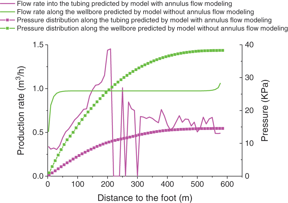
Figure 14: Profiles of pressure distribution and flow into the tubing (or along the wellbore) for the first case calculated using the two flow models for the ICD in the CMG simulator

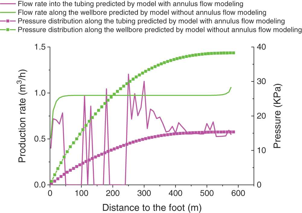
Figure 15: Profiles of pressure distribution and flow into the tubing (or along the wellbore) for the second case calculated using the two flow models for the ICD in the CMG simulator

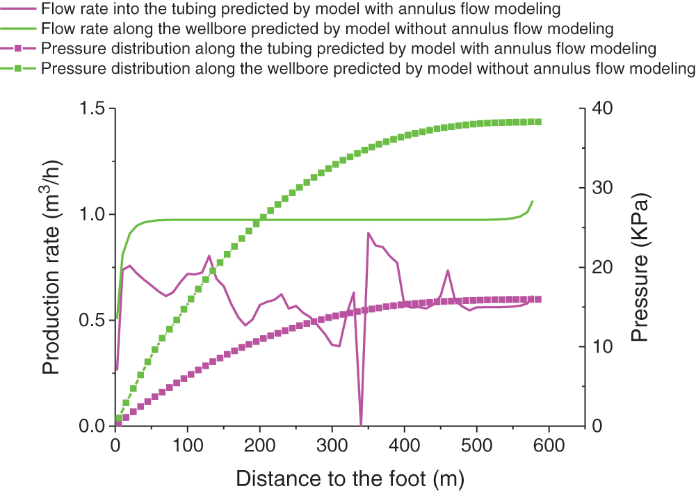
Figure 16: Profiles of pressure distribution and flow into the tubing (or along the wellbore) for the third case calculated using the two flow models for the ICD in the CMG simulator

Figs. 5, 6, 12 and 13 show the simulation results of the steady-state model established in this paper, and the calculation results are smoother. Figs. 11, 14–16 show the results of transient simulation using CMG simulation software. The inflow of some parts is the result of transient changes. During the transient change, at the next time point, this part will become another result, so Figs. 14–16 provide three graphs at different times. It can be seen from the graphs that the flow of a certain part at different times changes, but the overall curve trend is the same. That is, the closer to the heel end, the greater is the flow per unit length of the central tubing from the annulus.

4  Conclusions

Based on the principles of mass conservation and momentum conservation, a coupling model considering the variable mass flow of the central tubing, the variable mass flow of the annular tubing and the reservoir seepage was established to simulate the wellbore–annulus–reservoir state in a horizontal section of a slotted screen completion and ICD completion. This model is different from the previous coupling model that only considered central tubing variable mass flow and reservoir seepage flow. It has been compared with flow models without annulus flow. The following conclusions are drawn.

(1) If extra pipe packers are not considered, then for the completion of a slotted sieve tube well, the predicted yield of the variable mass flow model without annulus flow modeling is 9.51% higher than that of the variable mass flow model with annulus flow modeling; for an ICD completion, the predicted yield of the variable mass flow model without annulus flow modeling is 70.98% higher than that of the variable mass flow calculation model with annulus flow modeling. The ICD completion has a higher error than the predictive results of the slotted screen completion, with and without considering annulus flow. Both models show that the horizontal pressure profile and flow profile of the borehole wall are more uniform in the wellbore–annulus–reservoir of horizontal wells.

(2) For real well completion, it is observed that, several packers outside the ICD completion of the well pipe will only reduce the error in the prediction results between the models with and without annulus flow modeling. The error between the models with and without annulus flow modeling remains significant when packers outside the pipe are considered. The exact error is related to the number and positions of packers outside the pipe, which can be studied further based on the model with annulus flow modeling.

(3) Considering the influence of annulus flow and establishing a model for the corresponding horizontal section with annulus flow modeling are necessary, regardless of the slotted screen completion or ICD completion of the well, as long as annulus flow is present in the horizontal section. The flow model with annulus flow modeling is the basis for accurately predicting horizontal well production and optimizing the design parameters of a slotted screen completion and ICD completion.

(4) The predicted flow profiles of the established models for a slotted screen completion and ICD completion are all consistent with those obtained using the CMG simulator. The closer to the heel end, the greater is the flow per unit length of the central tubing from the annulus.

Acknowledgement: Thanks to Luo Wei for serving as the corresponding author for the article.

Funding Statement: This work was supported by the Scientific Research and Technological Development Project of CNPC (2019D-4413).

Conflicts of Interest: The authors declare that they have no conflicts of interest to report regarding the present study.

References

 1.  Wang, J., Sun, J., Liu, D., Zhu, X. (2019). Production capacity evaluation of horizontal shale gas wells in fuling district. Fluid Dynamics & Materials Processing, 15(5), 613–625. DOI 10.32604/fdmp.2019.08782. [Google Scholar] [CrossRef]

 2.  Han, D., Kwon, S. (2020). Development and application of a production data analysis model for a shale gas production well. Fluid Dynamics & Materials Processing, 16(3), 411–424. DOI 10.32604/fdmp.2020.08388. [Google Scholar] [CrossRef]

 3.  Tang, Y., Erdal, O., Mohan, K., Cem, S., Turhan, Y. (2000). Performance of horizontal wells completed with slotted liners and perforations. Society of Petroleum Engineers. [Google Scholar]

 4.  Mohammadsalehi, M., Goodarzian, S., Asef, M. R. (2010). Non-uniform slotted liner completion, a new approach to obtain uniform production profile along horizontal wells. American Journal of Orthodontics and Dentofacial Orthopedics: Official Publication of the American Association of Orthodontists, Its Constituent Societies, and the American Board of Orthodontics, 137(6), 796–800. [Google Scholar]

 5.  Wang, Q., Liu, H. Q., Zhang, H. L., Zheng, J. P. (2011). An optimization model of completion strings with inner-located nozzle in horizontal wells coupled with reservoirs. Acta Petrolei Sinica, 32(2), 346–349. [Google Scholar]

 6.  Zhao, X., Yao, Z. L., Liu, H. L. (2013). Technical research on well completion design with inflow control device (ICD) in horizontal wells. Oil Drilling & Production Technology, 35(1), 23–27. [Google Scholar]

 7.  Chen, Y., Peng, Z. G., Wang, S. X., Zhang, J. G., Zhang, L. et al. (2015). A new numerical coupling model of horizontal well completed with flow control method in bottom water reservoir. Journal of China University of Petroleum: Natural Science Edition, 39(6), 110–117. [Google Scholar]

 8.  Yang, Q. S., Liu, L., Wang, Z. M., Xiao, J. (2015). Study on reservoir seepage and wellbore flow in horizontal well completion with inflow control device (ICD). Journal of Yangtze University (from Science Edition), 12(14), 55–60. [Google Scholar]

 9.  Valvatne, P. H., Serve, J., Durlofsky, L. J., Aziz, K. (2003). Efficient modeling of nonconventional wells with downhole inflow control devices. Journal of Petroleum Science & Engineering, 39(1–2), 99–116. DOI 10.1016/S0920-4105(03)00042-1. [Google Scholar] [CrossRef]

10. Neylon, K., Reiso, E., Holmes, J., Nesse, O. B. (2009). Modeling well inflow control with flow in both annulus and tubing. SPE Reservoir Simulation Symposium. [Google Scholar]

11. Luo, W., Li, H. T., Wang, Y. Q., Wang, J. C. 2015a. A new semi-analytical model for predicting the performance of horizontal wells completed by inflow control devices in bottom-water reservoirs. Journal of Natural Gas Science and Engineering, 27(4), 1328–1339. DOI 10.1016/j.jngse.2015.03.001. [Google Scholar] [CrossRef]

12. Luo, W., Li, H., Wang, Y., Wang, J., Yang, M. (2015). Optimization of the number of openhole packers in horizontal wells completed by inflow control devices for different types of reservoirs. Journal of Engineering Research, 3(1), 81. DOI 10.7603/s40632-015-0009-4. [Google Scholar] [CrossRef]

13. Lorenz, M. D., Ratterman, E. E., Augustine, J. R. (2006). Uniform inflow completion system extends economic field life: A field case study and technology overview. Society of Petroleum Engineers. [Google Scholar]

14. Luo, W., Liao, R. Q., Wang, X. W., Yang, M., Qi, W. L. et al. (2018). Novel coupled model for productivity prediction in horizontal wells in consideration of true well trajectory. Journal of Engineering Research, 6(4), 1–21. [Google Scholar]

15. Xiong, Y. M., Pan, Y. D. (1997). Study on productivity prediction of the horizontal wells with the open hole series of completion methods. Journal of Southwest Petroleum University (Natural Science Edition), 19(2), 42–46. [Google Scholar]

16. Zhang, W. L. (2013). The application of ICD in oil rim for improving the production performance of horizontal wells. (Ph.D. Thesis). Northeast Petroleum University, China. [Google Scholar]

17. Liu, X. P., Guo, C. Z., Jiang, Z. X., Liu, X. G., Guo, S. P. (1999). The model coupling fluid flow in the reservoir with flow in the horizontal wellbore. Acta Petrolei Sinica, 20(3), 82–86. [Google Scholar]

This work is licensed under a Creative Commons Attribution 4.0 International License, which permits unrestricted use, distribution, and reproduction in any medium, provided the original work is properly cited.