Fluid Dynamics & Materials Processing

DOI: 10.32604/fdmp.2021.010974

ARTICLE

Effect of Patient-Specific Aorta Wall Properties on Hemodynamic Parameters

Mohamad Shukri Zakaria1,*, Haslina Abdullah2, Azmi Nordin1 and Syazwati Ahmad Zaki1

1Fakulti Kejuruteraan Mekanikal, Universiti Teknikal Malaysia Melaka, Hang Tuah Jaya, 76100, Malaysia
2Faculty of Mechanical & Manufacturing Engineering, Universiti Tun Hussein Onn, Parit Raja, 86400, Malaysia
*Corresponding Author: Mohamad Shukri Zakaria. Email: mohamad.shukri@utem.edu.my
Received: 11 April 2020; Accepted: 14 December 2020

1  Introduction

Aorta is the largest artery in the human body. The function of the aorta is to transport blood from the heart to the entire body, including the brain. There are diseases related to the hemodynamics of blood flow; these include blood clotting, arterial stenosis, high blood pressure, aneurysm, stroke, and abnormal heart rhythm. Such diseases are caused by abnormal hemodynamic blood flow in the aorta due to excess pressure, low effective stress at the aorta wall, and varying shear stress of the wall [1].

Invasive surgery and medication are ways to treat such diseases; however, these treatments have limitations. For example, the side effects of the treatment may cause internal organ malfunction (e.g., kidney), or even death [2]. Furthermore, blood clotting in the aorta is due to atherosclerotic plaque. Plaque accumulates on walls of the aorta and reduces the nominal diameter of the artery, thereby increasing blood velocity. When blood passes an obstructed region at high velocity, wall shear stress activates the platelets that cause the formation of a blood clot. Blood clots in the aorta may flow to the brain and block the artery [1], thereby causing a stroke. The study of hemodynamics is conducted to observe the effects of blood flow in the cardiovascular system to find solutions that treat the disease without side effects.

Computational Fluid Dynamics (CFD) modelling is widely used to solve many engineering problems; for example, in the design and manufacturing of aircraft, marine technology technology [3,4], electronic cooling, and, recently, in the biomedical field [5]. Over the last decade, CFD has been used to study the basics of hemodynamic flow inside the aorta [6–12]. Abnormal blood flow such as laminar, turbulent, and transient flow are observed to determine the cause of the disease and how to overcome it using CFD. Besides, the hemodynamic details of blood comprising physical, structural, vibration and fluid dynamics at the wall of aorta are ascertained using Fluid-Structure Interaction (FSI) simulation [13,14]. It allows to discern between rigid and flexible aorta in any condition, and complex geometrical areas can be observed. Besides, a comparison of the hemodynamic flow between rigid and flexible aorta is required to understand which is better for detecting blood clotting in the aorta.

The effects of aorta wall movements need to be incorporated into the FSI solver. FSI is becoming significant for studying arterial radial displacement, von misses stress and wall shear concerning the force of the fluid. An understanding of the FSI of the cardiovascular system using the CFD method is necessary for studying the effects of blood flow patterns, such as laminar, turbulence, steady and unsteady flow inside the aorta. There are several aspects between the fluid and wall that will be observed. Some of these include outer velocity at the aorta, boundary condition, flow pattern type, and pressure.

Velocity profile leads to friction between the fluid and the aorta, which is related to fluid viscosity. The flowing fluid creates a friction-based tangential force which is referred to as wall shear stress (WSS). WSS is a vital flow characteristic and can be directly measured through the computational method [15,16]. There is varying velocity near the aorta wall that affects WSS, and any changes can be measured. Furthermore, the deformation and/or movement of the arterial wall might impact WSS. This is because the velocity profile depends on wall movement. An increase in velocity leads to blood clotting inside the aorta, whose walls are sensitive to any changes in flow rate. Consequently, a high WSS value leads to the formation of atherosclerotic and large-sized bulges in the aorta [17]. Flexible and rigid wall simulations were used to observe the difference in WSS and velocity profile at both types of walls to see which form leads to the formation of a large-size atherosclerotic bulge.

In-vivo measurement for calculating WSS is limited by spatial resolution. Therefore, the flow field was used to calculate WSS. Any error in geometry affects WSS because the simulation is dependent on the geometry [18]. Wall shear stress is the primary aspect that leads to the formation of atherosclerotic plaque [19,20]. Besides, the surrounding wall shear stress changes because of an increase in the tensile stress at the plaque site.

Previous studies indicate that WSS corresponding to rigid wall simulation is higher compared to the FSI simulation [21]. The total pressure drop specific to the rigid aorta is also higher compared to a flexible aorta [22]. Although the flexible aorta closely mimics the real condition, the rigid model has the advantage of indicating the formation of another recirculation which cannot be seen in the MRI and FSI models [18]. Besides, the effects of wall shear stress specific to the rigid and flexible wall helps determine the endothelial function and decide near-wall details [23,24].

In the present study, the effects of wall behaviour on WSS were investigated and compared using the CFD and FSI methods. It is understood that the study, using simplified modelling techniques, will provide insight regarding the impact of material wall properties on valvular heart disease.

2  Methodology

CFD and FSI methods were employed as tools for developing and testing the mathematical model. ANSYS fluid dynamics and structural mechanics software was used for solving the model. The patient image was acquired using digital subtraction angiography. The image was reconstructed using image segmenting software.

2.1 Mathematical Model

A governing equation will be used by assuming that blood is an incompressible fluid having constant density. The assumption of blood having Newtonian properties was adequate where the blood vessel is considered larger compared to the size of the blood cells. The governing equation measures five quantities, namely, blood flow pressure, density, and three components of velocity. Blood velocity is determined for three axes, which are x-axis, y-axis and z-axis. In order to represent the average amount of element at a point on the surface, a fluid element had been used.

Blood flow inside the arteries has a dynamic effect on the aortic wall. Since blood is assumed to be a Newtonian fluid and the aortic wall is assumed to have an elastic structure, 3D FSI of the aorta was used to simulate hemodynamic parameters corresponding to the inside of the aorta. Besides, for solid simulation, the wall was assumed to have a rigid structure. The expression for FSI simulation is specified in Eqs. (1)–(6), where Eqs. (1)–(4) are the governing equations for blood flow, while Eqs. (5) and (6) are the governing equations for the solid wall of the aorta.

where ρ denotes blood density and denote the velocity components of blood flow in the x, y and z-direction, respectively.

The fluid solver for blood domain used in the present study are incompressible Navier-stokes equation shown in Eqs. (1)–(4). The convection term in momentum equation is solve using second order upwind was used to interpolate the face values of the various quantities from cell centre values and to ensure the stability. The diffusion terms are central differenced and second-order accurate. The diffusion terms are central differenced and second-order accurate. The PISO algorithm [25] was used to relate the pressure to the velocity. The discretized equations were then solved sequentially using a segregated solver. The simulation are running until convergence criteria reach below 10−6.

For the structural solver, the motion of an elastic solid is mathematically described by the equations shown below:

where u denotes the displacement vector of the solid wall, ρw is the wall density and Bi are the components of body force acting on the solid while and are Lame’s coefficients and related to Young’s modulus and the Poisson ratio as follows:

In the present simulation, Poisson’s ratio is 0.4998 and density is 1,121 kg/m3, which are properties representative of linear elastic material [22].

The FSI method works using two-way coupling between the fluid solver and the mechanical solver. The force magnitude obtained from fluid solver is input to the solid solver as a boundary condition. Subsequently, the displacement obtained by the solid solver is input to the fluid solver as a boundary condition.

2.2 Aorta Model

The aorta model implemented in this study is based on real-life patient-specific data concerning stenosis patients that were obtained from another author’s work [6]. The model comprises one inlet and four outlets, as shown in Fig. 1. This model was used for both conditions, namely rigid and flexible wall. For analysis, the minimum diameter of the aorta was chosen as 1 mm [22], and this approximation was acceptable.

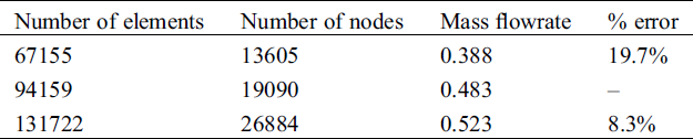
For the grid-independent test, three different number of element was used, which are 67166, 94159, and 131722 as shown in Tab. 1. The grid quality is determined by using 0.1 of ratio in number of gaps across cell and transition ratio in inflation. Finally, the model meshed into 94,159 elements and 19,090 nodes as the error for the mass flowrate were less than 10%. The method in calculating the error was conducted by referring to [26].

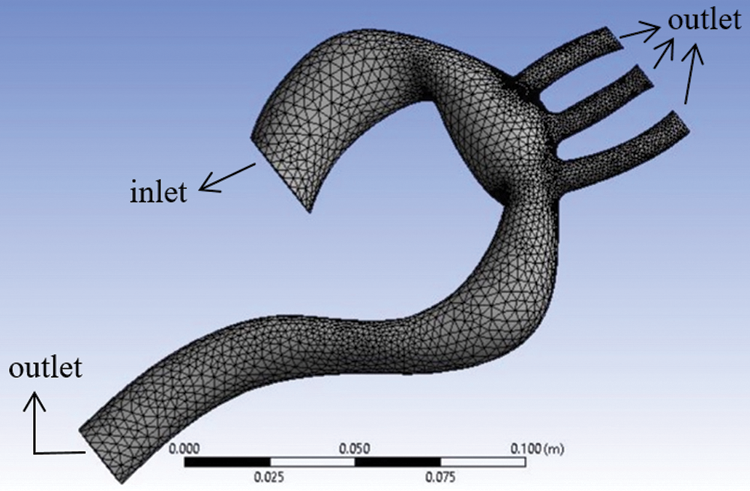
Figure 1: Aorta model showing the meshing and boundary conditions

Table 1: Mesh sensitivity analysis

The simulation was conducted using the ANSYS software package. The flexible wall simulation was a combination of Fluid Fluent and Static Structural aspects with the wall having linear elastic stiffness, and its Young’s Modulus assumed as 0.4 MPa [27]. At the same time, the rigid wall simulation was the only one considered for the fluid flow solver since there are no domains for the solid.

The boundary condition for the inlet velocity for both rigid wall and FSI simulation was assumed as steady 1 m/s, and the inlet pressure was assumed as 0 Pa. At the same time, the other four outlets were set at 0 Pa pressure. The boundary condition for rigid wall simulation assumed a stationary wall with a no-slip shear condition; for the flexible wall, the boundary condition was motion wall. The maximum value of Reynold’s number of the aorta was 1054, which is indicative of laminar flow. Reynold’s number was calculated based on the hydraulic diameter at the inlet.

3  Result and Discussion

3.1 Velocity

Figs. 2a and 2b represent the velocity for rigid and flexible aorta, respectively. The result shows that the highest velocity is at the aortic arch and the descending aorta. The result was also validated by the work from [6], in which the error in maximum velocity is 13%. The Aortic arch is the main artery between the ascending and descending aorta. The highest blood velocity is at the descending aorta, which carries blood to the legs. Besides, blood flows with high velocity at the aortic arch because it needs to flow through three smaller arteries, namely, the brachiocephalic artery, the left common carotid artery, and the left subclavian artery. The smaller arteries like the brachiocephalic artery, the left common carotid artery, and the left subclavian artery carry blood from the base of the neck to the brain.

Comparing between the results in Figs. 2(a) and 2(b), it can be observed that the maximum velocity for the walls is different; the maximum velocity at the flexible wall is 2.52 m/s and velocity at the rigid wall is 2.292 m/s at the BA, LCA and LSA, with a percentage difference of 9%. There was a minute difference in velocity at the descending aorta for the two walls. It is observed that the velocity at the descending aorta of the rigid wall decreases from 1.528 to 0.764 m/s. Besides, for flexible aorta, the velocity was 1.528 m/s.

Such phenomena happen because there was no motion at the wall. Blood flows due to gravity, and there is a decrease in blood velocity. Compared to the results of [22], the velocity decreased from 4.5 m/s to 2.7 m/s at the descending aorta for the rigid wall. At the same time, for the flexible wall, the velocity decreased from 4.0 m/s to 2.5 m/s. Furthermore, the recirculation corresponding to the flexible aorta is higher, as seen due wall movement at the ascending aorta.

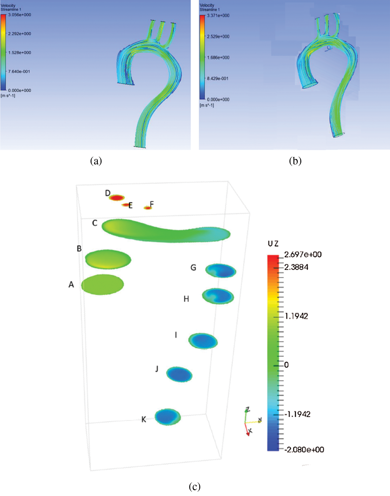
Figure 2: Velocity distribution for (a) rigid aorta and (b) flexible aorta (c) previous study [6]

Fig. 3 depicts the velocity contour corresponding to the ascending aorta, aortic arch, BA, LCA, LSA, and descending aorta. It shows that different locations of the aorta have different velocity. The velocity contours are also different for the rigid and flexible wall. The maximum velocity for the rigid wall was 2.333 m/s at the aortic arch, compared to 2.372 m/s at the descending aorta at the flexible wall. The average blood flow velocity to the leg was 1.3 m/s for the rigid wall, while for the flexible wall, the average velocity was 1.65 m/s at the descending aorta. The velocity at the smaller arteries is approximately similar for both walls, especially at the BA.

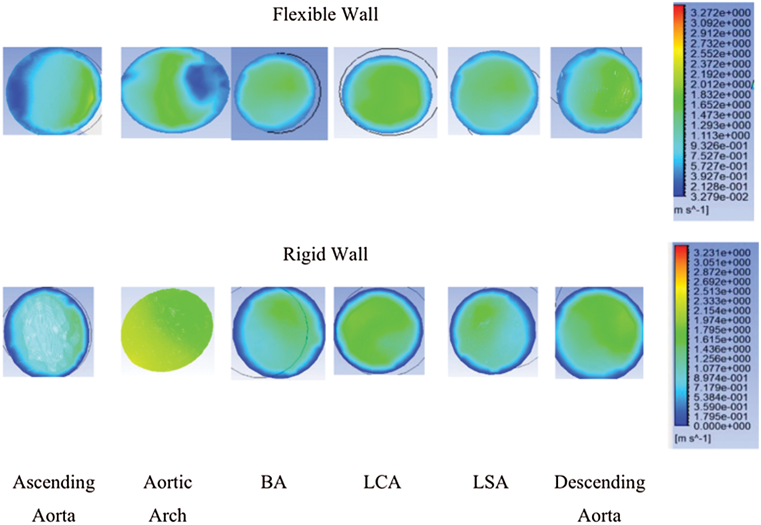
Figure 3: Velocity contour at ascending aorta, aortic arch, BA, LCA, LSA, and descending aorta

3.2 Pressure Distribution

Pressure contour corresponding to the ascending aorta was highest compared to the aortic arch, descending aorta, brachiocephalic artery, left common carotid artery, and left subclavian artery; there is a gradual decrease in blood flow, as shown in Fig. 4. The rigid wall aorta is seen having higher maximum pressure compared to the flexible wall aorta with a 0.253 kPa or 6.2% difference.

The difference between inlet and outlet pressure at the flexible wall was 1548.9 Pa compared to 1559 Pa for the rigid wall. It shows that the difference between inlet and outlet pressure for the rigid wall was higher compared to the flexible wall. Compared to work of [22], the difference in pressure for the rigid wall was also higher compared to the flexible wall, thereby indicating that the results obtained from the simulation in the current study were in agreement with previous research [22].

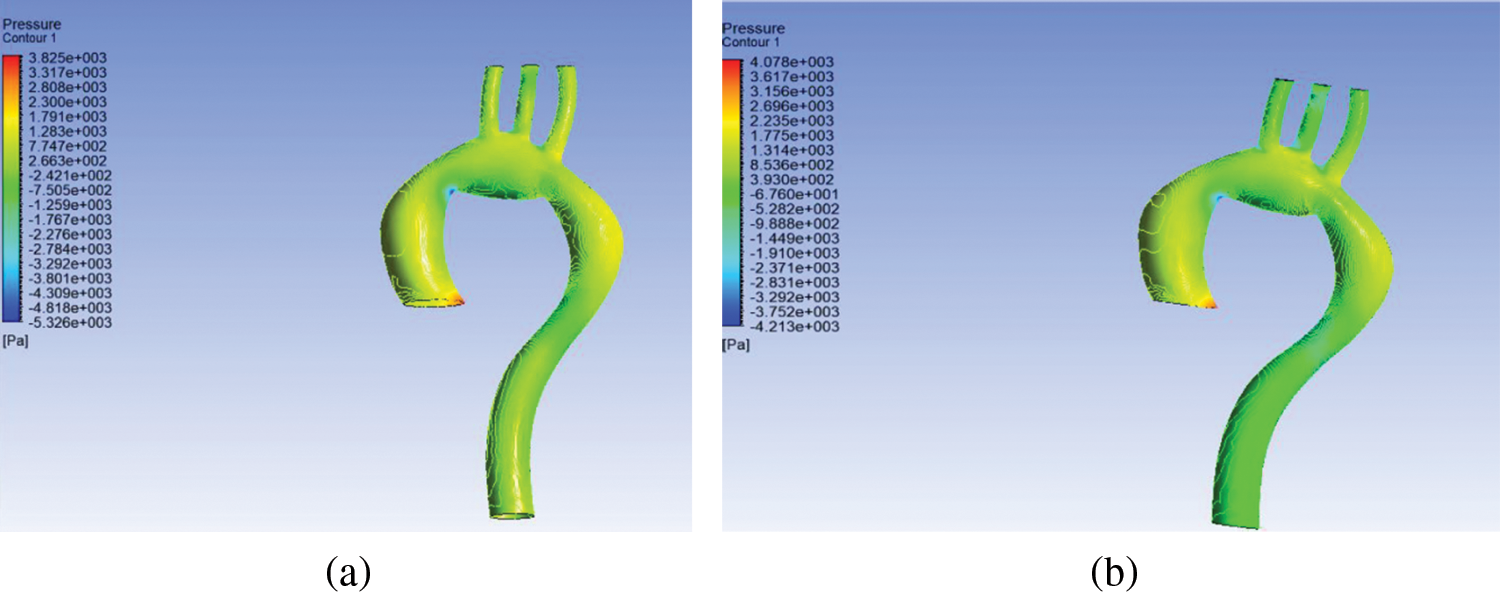
Figure 4: Pressure distribution at (a) flexible and (b) rigid wall aorta

3.3 Wall Shear Stress

The result of FSI showed that smaller arteries like brachiocephalic artery (BA), left common carotid artery (LCA), and left subclavian artery (LSA) have the highest WSS compared to a different arch of the aorta. Wall shear stress is high because of the blood flow through the smaller arteries like brachiocephalic artery and left common carotid artery. Comparing to the work by [27], it can be concluded that the high WSS value at the smaller arteries is in agreement.

Contrasting flexible and rigid aorta, it can be observed that the rigid wall has high WSS compared to the flexible aorta; however, the difference in WSS is minimal at about 5.98 Pa at the smaller arteries. The results specific to WSS are in agreement with the work of [18], where the WSS difference at the smaller arteries is small.

Furthermore, based on Figs. 5(a) and 5(b), it can be seen that the ascending descending aorta are more amenable to particle deposition and, consequently, worsening of the stenosis problem [22]. Moreover, at the edge of the aorta and smaller arteries, namely, BA, LCA, and LSA, there is a chance of aneurysm formation. Both diseases cause blood clotting and are dangerous to human health because clots can cause stroke when they reach the brain.

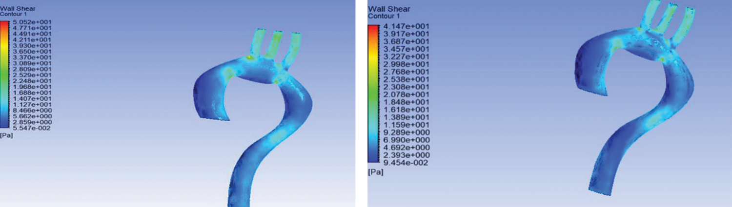
Figure 5: Wall shear stress for (a) rigid wall and (b) flexible aorta

4  Conclusion

In this research, hemodynamic parameters of flexible and rigid walls were observed for the real human aorta. CFD and FSI simulations were used to measure pressure, velocity, and WSS for the arteries; it is difficult to measure these parameters in-vivo or using medical tests. It was found that rigid aorta is more sensitive to hemodynamic parameters like high WSS and pressure drop. A higher value of WSS leads to cardiovascular diseases like haemolysis, thrombosis, and stenosis. For the numerical simulation that involves ascertaining the hemodynamic parameter for cardiovascular diseases, the rigid wall is assumption is considered to be the safest. It is recommended that future works consider modelling blood cell particles and take into account the damage on the individual cell that can be measured through FSI simulation.

Funding Statement: The authors wish to thank the Faculty of Mechanical Engineering at UTeM for its practical support and the Universiti Teknikal Malaysia Melaka (UTeM) and the Ministry Education Malaysia (MOE) for funding this research project through Grant No. FRGS/2018/FKM-CARE/F00367.

Conflicts of Interest: The authors declare that they have no conflicts of interest to report regarding the present study.

This work is licensed under a Creative Commons Attribution 4.0 International License, which permits unrestricted use, distribution, and reproduction in any medium, provided the original work is properly cited.