Fluid Dynamics & Materials Processing

DOI: 10.32604/fdmp.2021.010376

ARTICLE

On the Efficiency of a CFD-Based Full Convolution Neural Network for the Post-Processing of Field Data

Sheng Bai, Feng Bao*and Fengzhi Zhao

School of Computer and Information Technology, Northeast Petroleum University, Daqing, 163318, China
*Corresponding Author: Feng Bao. Email: ruya2003@163.com
Received: 19 March 2020; Accepted: 18 December 2020

1  Introduction

Hydrodynamics deals with the motion of fluids and the forces acting on solid bodies immersed in fluids and in motion relative to them [1]. Computational fluid dynamics (CFD) is a branch of hydrodynamics developed as computer science and aerospace industry advance. CFD can simulate and analyze the motion of fluids [2], applied to molecular motion, heat exchange, fluid flow, environmental engineering, and water conservancy engineering fields. Traditional CFD methods are accurate and precise but slow in the calculation. Besides, they cannot fully utilize the calculation results, which hinders the aircraft design and even restricts the manufacturing industry’s development. Academia has researched the acquisition and application of CFD data. Some scholars established the third-order CFD database through CFD simulation, a novel way to reconstruct the wind speed distribution in 3D space [3]. Some researchers used 3D CFD data to calculate the attack angle and the induced velocity of the wind turbine blade’s underlying surface, which could calibrate the blade element momentum tool [4]. Some researchers studied the reactor of Hot Wire Chemical Vapor Deposition (HWCVD) using the CFD framework and determined the safe deposition distance in the HWCVD reactor [5]. Many studies discuss accelerating CFD’s calculation process, such as the launch of FLUENT15.0 accelerated version, a commercial CFD calculation software in 2014, and the combination of a Field-Programmable Gate Array (FPGA) and a Central Processing Unit (CPU). The flow field describes the spatial distribution of fluids’ motion. The flow field data describe fluid particles’ motion data, including density, temperature, pressure, viscosity, and velocity, using the Euler method [6,7]. These data can record fluid particles’ motions and describe the fluid motion’s spatial distribution [8]. As technology advances, the complexity of flow field data increases. Consequently, requirements for calculation accuracy, data analysis, and data processing also raise, making traditional methods inapplicable. In summary, optimizing flow field data processing is an urgent problem.

AlexNet proposed in 2012 and ResNet proposed in 2015 are representative deep learning models. Such models have strong classification and recognition abilities, in which neural networks are accurate and fast. Convolutional Neural Network (CNN), a traditional semantic segmentation method, operates slowly and occupies a large space [9–11]. As an improvement, the Fully Convolutional Network (FCN) can deconvolute CNN’s results. Hence, each pixel’s classification prediction is reversely recovered from the convolution extraction features, thereby improving the semantic segmentation efficiency. FCN has applications in various fields, including vision tracking and edge detection [12,13]. CNN can judge the objects’ categories in the image while extracting abstract features. However, CNN cannot describe the objects’ contour features. FCN is formed by applying CNN to nonlinear fitting functions and using nonlinear filters in each CNN layer. FCN can recover the classification of each pixel from the abstract features and extend the image classification to pixel classification. Compared with CNN, FCN can detect all size input images, generate classification prediction for each pixel, and retain the image’s initial position information.

Moreover, the FCN’s detection methods are efficient, avoiding the repeated calculation and redundant storage caused by pixel blocks. It can classify the images and pixels as well. However, FCN has some defects, such as insufficient precision of the results, fuzzy feature information of the up-sampling, and no consideration of the spatial correlation among pixels. Still, FCN shows some advantages in the data processing.

In the present study, VGGNet (Visual Geometry Group Net) can overcome FCN’s limitations. First, the flow field data in aircraft design are post-processed. Then, the simulation regression model for flow field data, FCN-VGG19, is established. This model undergoes tests on the TensorFlow platform. The research results can provide a theoretical reference for processing flow field data using CFD, FCN, and VGGNet.

2  Methods

2.1 FCN Based on VGGNet

VGGNet deals with the relationship between CNN’s depth and performance. Compared with other networks, VGGNet can minimize the error rate [14,15]. VGGNet uses a 3 × 3 convolution kernel and a 2 × 2 pooling layer to construct CNN (containing 6 to 19 layers). VGGNet has five convolution sections, and each section contains two or three convolutional layers. These convolutional layers have small filters and intervals. The image size is changed by connecting the maximum pooling layer after each section of the convolutional layer, which has strong feature learning capability. After several iterations, the network converges, while the operating speed does not decrease. As flow field data become complicated, requirements on flow field data post-processing will rise. In aircraft design, CFD methods can simulate the flight of aircraft, which is pretty essential. However, traditional CFD methods take much time in calculation. Thus, a simulation regression model of flow field data is established based on FCN. The image processing method under deep learning simulates the calculation process of flow field data. A 19 layers-based VGGNet can apply to FCN, recorded as FCN-VGG19. The calculation model of flow field data based on FCN-VGG simulates the regression calculation of flow field data in aircraft design. Fig. 1 shows the calculation process.

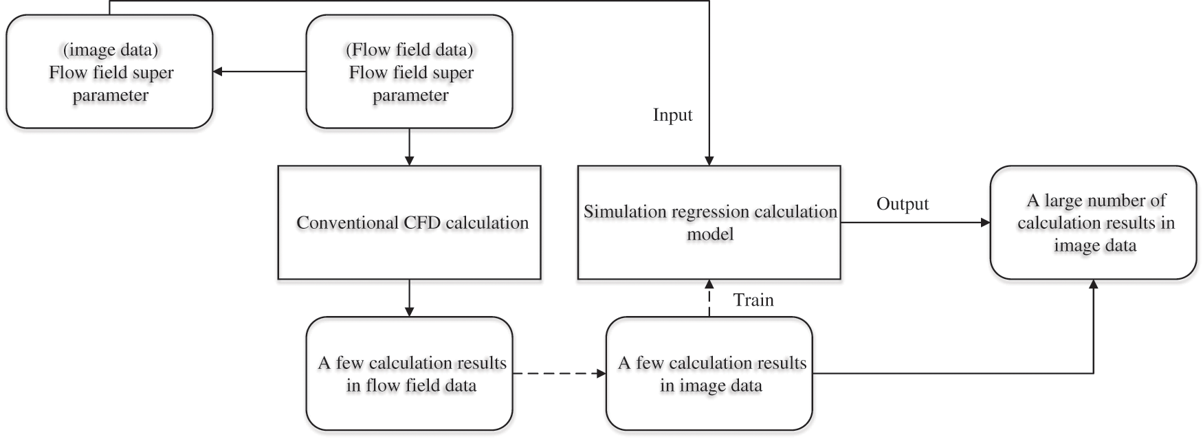
Figure 1: FCN-VGG’s calculation process

2.2 TensorFlow Deep Learning Platform

Google Inc. developed TensorFlow, a platform with high-quality codes and excellent design architecture. TensorFlow supports Python that is mature in data mining, and each of its databases is excellent. TensorFlow and Python are linked correctly during model training [16]. TensorBoard, TensorFlow’s visual Web program, can monitor its running process. Visual parameters in TensorBoard are critical. The results after several iterations and the display platform’s calculation process can be predicted by saving images needed in the operation process. TensorFlow provides a sound precondition for building the model, saving the visualization time during coding [17,18]. Thus, the TensorFlow deep learning platform builds the model for the aircraft’s flow field data post-processing. The first several layers of FCN-VGG19 are the VGG networks, containing six convolutional layers and two pooling layers. The convolution kernel in the convolutional layer is 3 × 3. Through average pooling function, image size can shrink by 32 times after five pooling layers. The sixth to eighth layers are single convolutional layers with 7 × 7 convolutional kernels. In these layers, the image size will not change. The last three deconvolutional layers restore the image size for using the detailed image features during deconvolution. A single-channel image with the same size can be output as the original image after 19 convolution calculations and three deconvolution calculations. The target observation variables’ distribution and changes are output as pressure, air density, and air velocity. Various grid segmentation methods record the aircraft’s flow field distribution during flight. The flight velocity, altitude, attack angle, and sideslip angle of the aircraft are super parameters of the flow field data. The reference criterion of high importance pressure P is the observation variable. The input and output layers of FCN-VGG are modified. TensorFlow constructs the network architecture, and Python is the programming language. Fig. 2 shows the simulation regression calculation model of flow field data based on FCN.

In this model, the first step is to train the FCN-VGG19 network based on CFD calculation. The regression calculation model can effectively simulate CFD’s calculation process in a particular flow field. This step completes most CFD calculation processes, accelerating the CFD calculation. Then, the trained model can generate flight images under flight conditions.

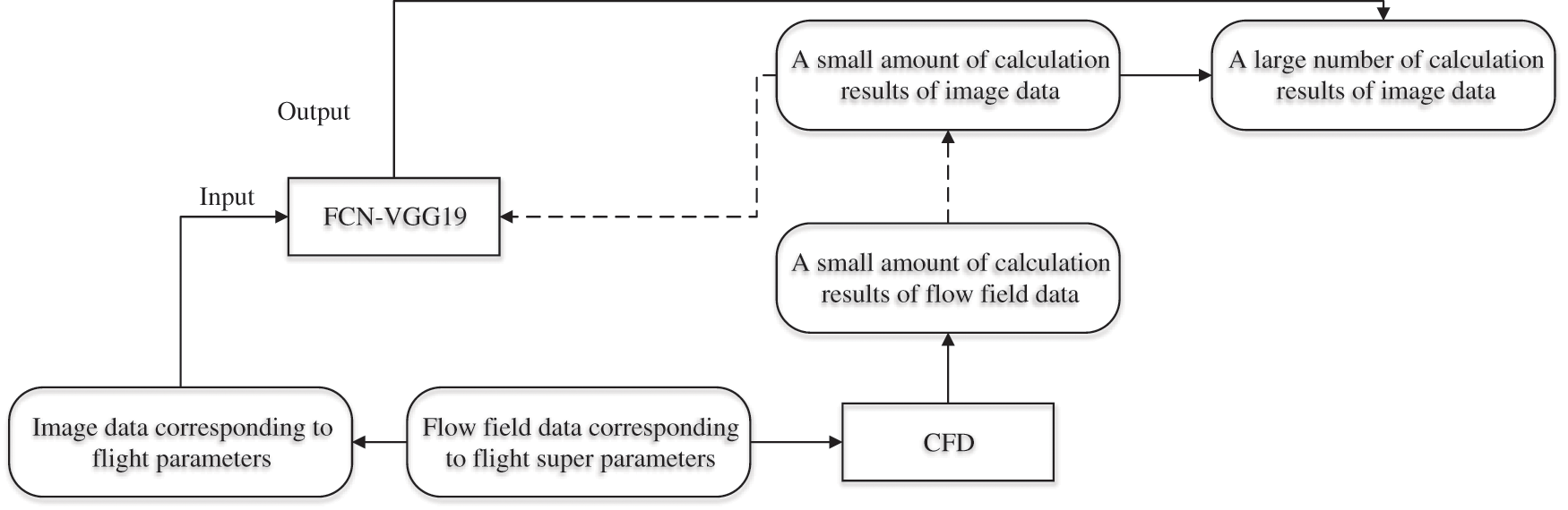
Figure 2: Simulation regression model of flow field data based on FCN-VGG19

2.3 Evaluation Criteria of Flow Field Calculation Model

Different target observation variables, and the same target observation variable under different grids, are used in the same grid when evaluating the regression calculation model’s prediction results based on FCN. This process investigates and evaluates the influence of different grids and different target observation variables on the simulation regression calculation model’s generalization performance. The applicability of different aircraft flow field data in the simulation regression model is verified and evaluated. Under the same grid, the apparent pressure, air density, and air velocity expressed in the data results are the target observation variables, which train and verify the proposed model. The evaluation and prediction criteria are: Mean Absolute Error (MAE), Mean Square Error (MSE), and R-square determination coefficient [19–22]. MAE is the mean corresponding to the absolute residual value, and MSE is the mean corresponding to the square residual value, also known as L2 loss. MSE can be biased and unbiased according to the correspondence between the expected value and the true value. The proposed model predicts the overall image’s MSE. The R-square coefficient can be a criterion for comparing the same model in different datasets. In the present study, the R-square determination coefficient is re-defined. The mathematical definitions of MAE, MSE, L2 loss, and the re-defined R-square determination coefficient are Eqs. (1)–(4).

In (1), m represents the number of predictions, i and j represent the specific number of predictions.

In (2), n refers to the total prediction times, i represents the specific number of predictions, stands for the prediction results generated for the overall image, and y represents the initial image’s prediction results.

In (3), n refers to the total prediction times, m indicates the side length of the image, i represents the specific number of predictions, is the pixel point’s prediction value in the k-th row and the j-th column, and y is the initial value corresponding to the position.

In (4), range(y) indicates the value range of y.

3  Results and Discussion

3.1 Calculation Model of Flow Field Data Based on FCN-VGG19

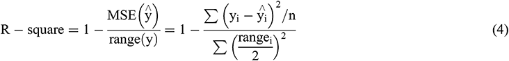
FCN-VGG is the primary network architecture of the proposed model. The aircraft design’s flow field structure and loss characteristics are analyzed. Fig. 3 shows the data results.

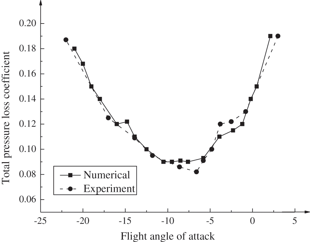
Figure 3: Changes between the angle of attack and the total pressure loss

The characteristics of the simulation calculation model, VGGNet, and FCN (Fig. 2) are combined. According to the flow field structure’s analysis results and the aircraft design’s loss characteristics, the model for calculating flow field data has good credibility. The FCN-VGG network has a robust fitting ability. The simulation regression model has high accuracy and strong convergence. FCN’s calculation process is intensive, which classifies and regresses the image pixels while putting forward the needs for high-level and detailed feature information. During the regression calculation, the activation function is not necessary for the classification. In the FCN-VGG19 network, the first deconvolution layer’s results for the eighth convolutional layer are deconvolution, and the feature map channel changes accordingly. The second deconvolution layer’s input corresponds to the results of the first deconvolution layer and the fourth convolutional layer. The third deconvolution layer’s input corresponds to the results of the second deconvolution layer and the third convolutional layer. The above image processing method for aircraft’s flow field data transforms flight data analysis into image data analysis. Then, it is applied to generate simulated flight images of aircraft design. The collected flight data is then adopted to train and evaluate the simulation regression calculation model based on FCN, thereby accelerating the design process of the simulation calculation and the visualization process of aircraft flight.

3.2 Simulation and Regression Calculation of Flow Field Data

The proposed FCN-based model is applied to generate simulated flight images in aircraft design to calculate and simulate the flow field data in aircraft design. Under the Linux operating system, the training model’s dropout rate takes 0.15 to analyze the input grid data and extract the feature information. The grid data size is transformed into 224 × 224 images; the L2 loss monitors the simulation regression process of aircraft flow field data in real-time. Fig. 4 shows the L2 loss changes in the simulation regression calculation model.

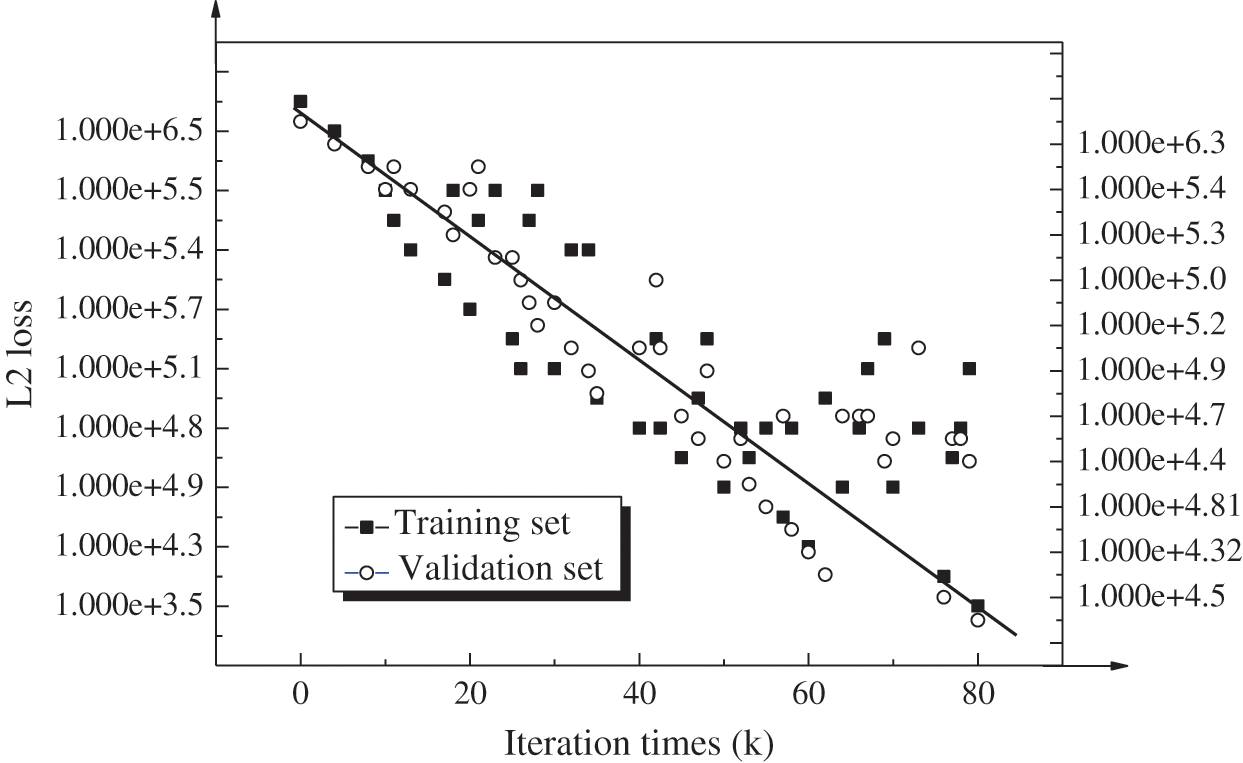
Figure 4: L2 loss changes of simulation regression calculation model

Changes in data information points suggest that L2 loss’s changing trend calculated in the training set is similar to that in the validation set during model training, without over-fitting. Changes in L2 loss will become stable after several iterations. The corresponding dataset’s prediction and regression will be trained. A visual image will be output every 100 iterations, and the corresponding dataset will be verified every 10 k iterations. When the number of training iterations exceeds 10 k, the model’s L2 loss is below 1 × 105 for the 224 × 224 flow field image.

Once CFD in the same flow field space is analyzed and calculated, the value distribution corresponding to the super parameters will always be uneven and dependent. However, in different CFDs’ calculation environments, super parameter selection varies significantly. A proper selection strategy for training samples is necessary for analyzing super parameters’ distribution characteristics. After 10 k training iterations of the model, target observation variables are simulated, calculated, and regressed under specific flight parameters. At this time, the simulation regression calculation model converges. The model fits the flight data excellently during this process, and the target observation variable P’s simulation regression effect is brilliant.

3.3 Evaluation of the FCN-Based Simulation Regression Calculation Model

The FCN-based simulation regression calculation model post-processes the flow field data of the aircraft. When the air density is the target observation variable, the training and verification processes of the proposed model are shown in Fig. 5 below. The airflow rate represents the target observation variable and the L2 loss changes in the “WALL-5” grid for comparative analysis. The training and verification processes of the model are shown in Fig. 6.

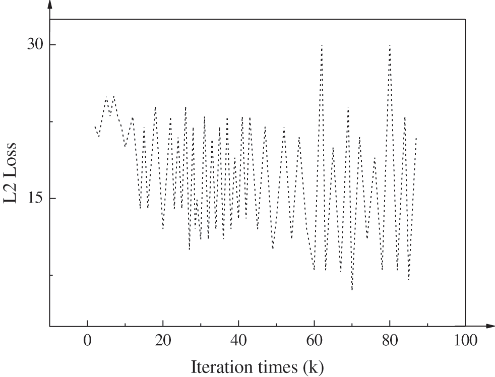
Figure 5: L2 loss change with air density as the target observation variable

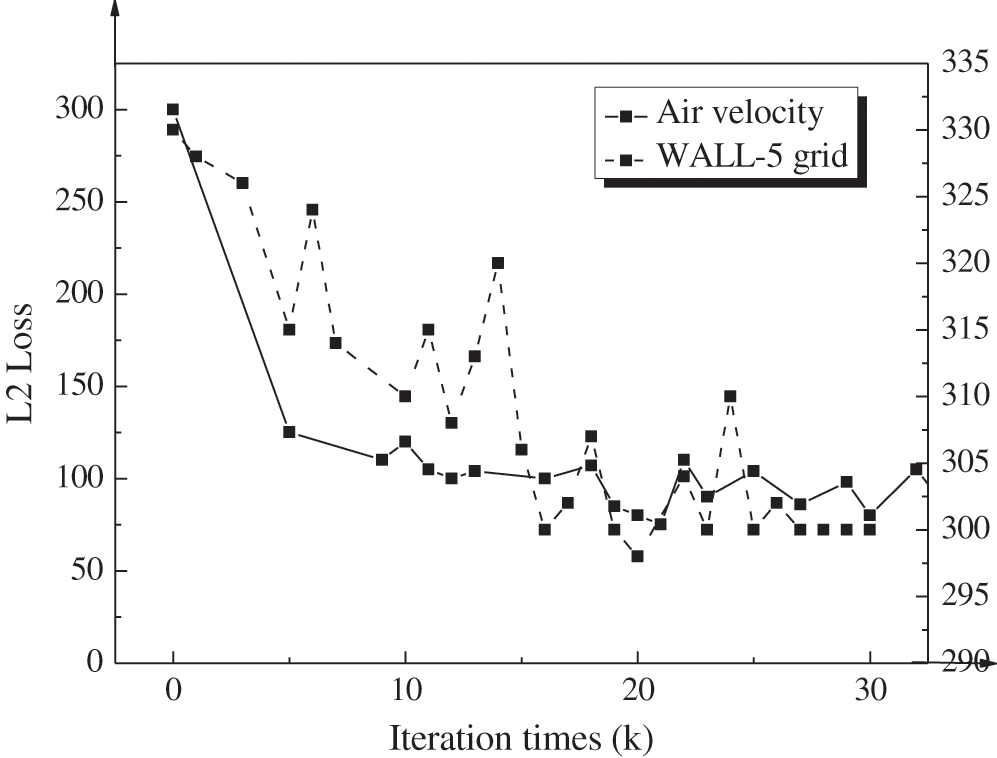
Figure 6: L2 loss change in air velocity and the “WALL-5” grid

Data changes in Figs. 4–6 are analyzed. Under the same grid, in pressure P’s prediction regression analysis, if the model’s training iterations exceed 10 k, the model’s L2 loss changes will become stable as a whole. L2 loss in the validation set is observed and analyzed. The calculated average MSE is 1.02 × 105 in the range of 10 k–80 k training iterations. Under the same grid, in air density’s prediction regression analysis, the model’s L2 loss becomes gentle when training iterations exceed 10 k. Within the same training iteration range as pressure prediction regression analysis, the air density’s MSE is 13.83, and air velocity’s MSE is 56.38. Data changes in Fig. 6 reveal that images’ MSE tends stable after 3k training iterations in the “WALL-5” grid’s prediction regression analysis with P as the target observation variable. Within the range of 3 k–30 k training iterations, the image’s MAE is 2.18. At this time, the R-square determination coefficient of the simulation regression calculation model is negative. Nevertheless, when the number of training iterations exceeds 20 k, the R-square determination coefficient is greater than 0.4, and the data fitting of the simulation regression calculation model meets the requirements.

Simulation regression for different target observation variables shows that the FCN-based model and the flight data fit well, and the model converges. Hence, the model’s generalization performance in different target observation variables is outstanding. In aircraft design, the observation variables are nature’s physical quantities with different physical characteristics, changes, distributions, and laws. Different observation variables have quite different value ranges. Without data standardization, the target observation variables’ value ranges will affect the regression calculation model. Therefore, predicting and evaluating the effect of the simulation regression model is necessary for different observation variables. When different grids are used as research objects, the difference in grids only shows that the model’s input images are different. However, the regression calculation on different grids has little impact. Thus, the only pressure is selected as the target observation variable for prediction regression analysis on the “WALL-5” grid. After several training iterations, the post-processing of aircraft’s flow field data fit well, showing that the model has generalization in different grids. Compared with the traditional calculation methods, the FCN-based simulation regression calculation model has accelerated calculation time. Furthermore, the model shows good generalization performance, which applies to various image and pixel regression calculation scenarios.

4  Conclusions

In the present study, flow field data in aircraft design are processed, FCN’s application and development are discussed, the modified VGGNet is applied to FCN, and the simulation regression calculation model for aircraft’s flow field data processing is established based on FCN-VGG19. According to L2 loss’s real-time monitoring results, the simulation regression calculation model is trained and tested on the TensorFlow deep learning platform using the Python programming language. Moreover, the simulation regression calculation model for the aircraft’s flow field data is evaluated according to the model’s generalization performance.

Parameters’ analysis and observation results show that the image processing method of flow field data based on FCN-VGG19 transforms flight data analysis into image data analysis. The established model has a strong fitting ability, high accuracy, and strong convergence. While predicting and constructing the model, the target observation parameter P is regressed after 10k model training iterations, and then the model converges. The simulation regression calculation model for aircraft’s flow field data presents high fitting performance for regressing different target observation variables and grids. The proposed model has good generalization performance for different target observation values and grids, which applies to the regression calculation of image pixels in various fields. However, the model does not investigate the relationship between flow field data processing and parameters, which will guide later research.

Acknowledgement: Acknowledgements and Reference heading should be left-justified, bold, with the first letter capitalized but have no numbers. The text below continues as usual.

Funding Statement: The author(s) received no specific funding for this study.

Conflicts of Interest: The authors declare that they have no conflicts of interest to report regarding the present study.

References

 1.  Benjemaa, M., Krichen, B., Meslameni, M. (2016). Fixed point theory in fluid mechanics: An application to the stationary navier-stokes problem. Journal of Pseudo-Differential Operators and Applications, 8(1), 1–6. [Google Scholar]

 2.  Boffetta, G., Mazzino, A. (2016). Incompressible rayleigh-taylor turbulence. Annual Review of Fluid Mechanics, 49(1), 119–143. DOI 10.1146/annurev-fluid-010816-060111. [Google Scholar] [CrossRef]

 3.  Zhang, C., Wu, M. (2019). An analysis of the stretching mechanism of a liquid bridge in typical problems of dip-pen nanolithography by using computational fluid dynamics. Fluid Dynamics & Materials Processing, 15(4), 459–469. DOI 10.32604/fdmp.2019.08477. [Google Scholar] [CrossRef]

 4.  Qin, L., Liu, S., Kang, Y., Yan, S. A., Schlaberg, H. I. et al. (2019). Wind velocity distribution reconstruction using CFD database with Tucker decomposition and sensor measurement. Energy, 167(15), 1236–1250. DOI 10.1016/j.energy.2018.11.013. [Google Scholar] [CrossRef]

 5.  Rahimi, H., Schepers, J. G., Shen, W. Z., Ramos García, N., Schneider, M. S. et al. (2018). Evaluation of different methods for determining the angle of attack on wind turbine blades with CFD results under axial inflow conditions. Renewable Energy, 125(9), 866–876. DOI 10.1016/j.renene.2018.03.018. [Google Scholar] [CrossRef]

 6.  Fourie, L. F., Square, L. (2020). Determination of a safe distance for atomic hydrogen depositions in hot-wire chemical vapour deposition by means of CFD heat transfer simulations. Fluid Dynamics & Materials Processing, 16(2), 225–235. DOI 10.32604/fdmp.2020.08771. [Google Scholar] [CrossRef]

 7.  Zubair, M., Riazuddin, V. N., Abdullah, M. Z., Ismail, R., Shuaib, I. L. et al. (2018). Airflow inside the nasal cavity: Visualization using computational fluid dynamics. Asian Biomedicine, 4(4), 657–661. DOI 10.2478/abm-2010-0085. [Google Scholar] [CrossRef]

 8.  Kumar, R., Kumar, A., Goel, V. (2017). A parametric analysis of rectangular rib roughened triangular duct solar air heater using computational fluid dynamics. Solar Energy, 157, 1095–1107. DOI 10.1016/j.solener.2017.08.071. [Google Scholar] [CrossRef]

 9.  Hsu, W., Daiguji, H. (2016). Manipulation of protein translocation through nanopores by flow field control and application to nanopore sensors. Analytical Chemistry, 88(18), 9251–9258. DOI 10.1021/acs.analchem.6b02513. [Google Scholar] [CrossRef]

10. Razavi, A., Sarkar, P. P. (2018). Laboratory study of topographic effects on the near-surface tornado flow field. Boundary-Layer Meteorology, 168(2), 189–212. DOI 10.1007/s10546-018-0347-5. [Google Scholar] [CrossRef]

11. Ma, Y., Cai, X., Sun, F. (2020). Towards no-reference image quality assessment based on multi-scale convolutional neural network. Computer Modeling in Engineering & Sciences, 123(1), 201–216. DOI 10.32604/cmes.2020.07867. [Google Scholar] [CrossRef]

12. Novikov, E. A., Sergeev, Y. A. (2019). Application of multidimensional analysis methods to dead oil characterization on the basis of data on thermal field-flow fractionation of native asphaltene nanoparticles. Petroleum Chemistry, 59(1), 34–47. DOI 10.1134/S0965544119010122. [Google Scholar] [CrossRef]

13. Liu, X., Zhao, D. (2017). P-wave anisotropy, mantle wedge flow and olivine fabrics beneath Japan. Geophysical Journal International, 210(3), 1410–1431. DOI 10.1093/gji/ggx247. [Google Scholar] [CrossRef]

14. Larsson, M., Zhang, Y., Kahl, F. (2018). Robust abdominal organ segmentation using regional convolutional neural networks. Applied Soft Computing, 70, 41–52. DOI 10.1016/j.asoc.2018.05.038. [Google Scholar] [CrossRef]

15. He, H. Q., Chen, T., Chen, M. Q., Li, D. J., Cheng, P. G. (2019). Remote sensing image super-resolution using deep–shallow cascaded convolutional neural networks. Sensor Review, 39(5), 629–635. DOI 10.1108/SR-11-2018-0301. [Google Scholar] [CrossRef]

16. Guo, H., Wu, X., Su, S., Fu, R. (2017). 3D background estimation for moving object detection using a single moving camera. Yi Qi Yi Biao Xue Bao/Chinese Journal of Scientific Instrument, 38(10), 2573–2580. [Google Scholar]

17. Zhou, Y. C., Xu, T. Y., Deng, H. B., Miao, T. (2018). Real-time recognition of main organs in tomato based on channel wise group convolutional network. Nongye Gongcheng Xuebao/Transactions of the Chinese Society of Agricultural Engineering, 34(10), 153–162. [Google Scholar]

18. Wang, Q., Gao, J., Yuan, Y. (2017). Embedding structured contour and location prior in siamesed fully convolutional networks for road detection. IEEE Transactions on Intelligent Transportation Systems, 99, 1–12. DOI 10.1109/TITS.2012.2219528. [Google Scholar] [CrossRef]

19. Saez, Y., Baldominos, A., Isasi, P. (2016). A comparison study of classifier algorithms for cross-person physical activity recognition. Sensors, 17(1), 66. DOI 10.3390/s17010066. [Google Scholar] [CrossRef]

20. Ansari, M. I., Anwer, S. F. (2018). Numerical analysis of an insect wing in gliding flight: Effect of corrugation on suction side. Fluid Dynamics & Materials Processing, 14(4), 259–279. DOI 10.32604/fdmp.2018.03891. [Google Scholar] [CrossRef]

21. Ihdene, M., Malek, T. B., Aberkane, S., Moderres, M., Spiterri, P. et al. (2017). Analytical and numerical study of the evaporation on mixed convection in a vertical rectangular cavity. Fluid Dynamics & Materials Processing, 13(2), 85–105. [Google Scholar]

22. Hamimid, S., Guellal, M. (2016). Thermomagnetic convection-surface radiation interactions in microgravity environment. Fluid Dynamics & Materials Processing, 12(4), 137–153. DOI 10.32604/fdmp.2016.012.137. [Google Scholar] [CrossRef]

This work is licensed under a Creative Commons Attribution 4.0 International License, which permits unrestricted use, distribution, and reproduction in any medium, provided the original work is properly cited.