
 Submit a Paper
 Propose a Special lssue
 Open Access
ARTICLE

Advanced Predictive Analytics for Green Energy Systems: An IPSS System Perspective
1 Electric Engineering Department, Huaian Hongneng Group Co., Ltd., Huaian, 223002, China
2 Faculty of Automation, Huaiyin Institute of Technology, Huaian, 223002, China
* Corresponding Author: Jie Ji. Email:
Energy Engineering 2025, 122(4), 1581-1602. https://doi.org/10.32604/ee.2025.061010
Received 14 November 2024; Accepted 20 January 2025; Issue published 31 March 2025
 View Full Text
 Download PDF
Abstract
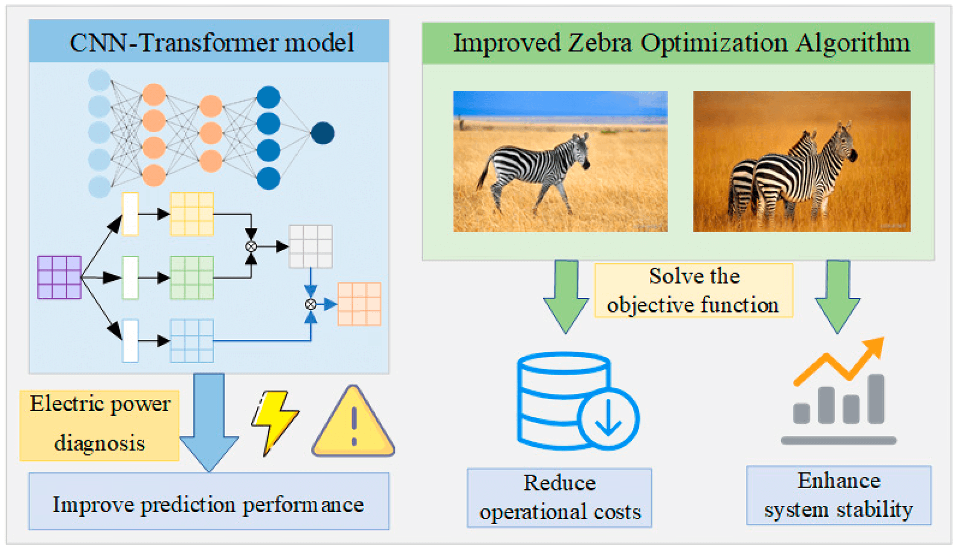
The rapid development and increased installed capacity of new energy sources such as wind and solar power pose new challenges for power grid fault diagnosis. This paper presents an innovative framework, the Intelligent Power Stability and Scheduling (IPSS) System, which is designed to enhance the safety, stability, and economic efficiency of power systems, particularly those integrated with green energy sources. The IPSS System is distinguished by its integration of a CNN-Transformer predictive model, which leverages the strengths of Convolutional Neural Networks (CNN) for local feature extraction and Transformer architecture for global dependency modeling, offering significant potential in power safety diagnostics. The IPSS System optimizes the economic and stability objectives of the power grid through an improved Zebra Algorithm, which aims to minimize operational costs and grid instability. The performance of the predictive model is comprehensively evaluated using key metrics such as Root Mean Square Error (RMSE), Mean Absolute Percentage Error (MAPE), and Coefficient of Determination (R2). Experimental results demonstrate the superiority of the CNN-Transformer model, with the lowest RMSE and MAE values of 0.0063 and 0.00421, respectively, on the training set, and an R2 value approaching 1, at 0.99635, indicating minimal prediction error and strong data interpretability. On the test set, the model maintains its excellence with the lowest RMSE and MAE values of 0.009 and 0.00673, respectively, and an R2 value of 0.97233. The IPSS System outperforms other models in terms of prediction accuracy and explanatory power and validates its effectiveness in economic and stability analysis through comparative studies with other optimization algorithms. The system’s efficacy is further supported by experimental results, highlighting the proposed scheme’s capability to reduce operational costs and enhance system stability, making it a valuable contribution to the field of green energy systems.Graphic Abstract
Keywords
In modern society, stable electricity supply is indispensable for almost all industries and daily life, ranging from household electricity to industrial production, from commercial operations to public services. The stable supply of electricity is the foundation for maintaining the normal operation of society. Therefore, ensuring the stability of electricity is not only the core objective of power system operation but also a key guarantee for the stable development of the social economy.
With the rapid development and increasing installed capacity of new energy sources such as wind and solar energy, the operational characteristics and structure of the power grid are undergoing significant changes. These changes bring new challenges to the fault diagnosis of the power grid. Firstly, the intermittency of wind and solar energy leads to drastic fluctuations in grid load, increasing the uncertainty of grid operation and making fault diagnosis more complex. Secondly, the integration of new energy into the grid poses higher requirements for grid stability and voltage control, necessitating more precise monitoring and diagnostic technologies to detect and handle potential faults in a timely manner. Liu et al. [1] proposed a dynamic vulnerability assessment method that addresses the uncertainty issues in the safety and stability of hybrid power systems by considering the random fluctuations of wind power. Eskandari et al. [2] introduced a comprehensive six-layer multilayer model that diagnoses, classifies, and identifies the severity of electrical faults in photovoltaic arrays, solving the problem of early detection of photovoltaic system faults to improve their service life and reliability. Ajagekar et al. [3] proposed a hybrid QC-based deep learning framework solving the issues of computational workload and diagnostic performance quality, and improving computational efficiency. Hao et al. [4] proposed a method for the operation status assessment and fault diagnosis of photovoltaic arrays based on an enhanced Adaptive Neuro-Fuzzy Inference System (ANFIS), which effectively improves the precision and stability of the evaluator by improving ANFIS, solving the problem of fault diagnosis in photovoltaic arrays.
Existing methods seldom apply predictive technology to fault diagnosis, and the application of predictive technology in fault diagnosis remains a relatively new and underutilized field. There is a wide variety of predictive technologies that cover multiple domains and scenarios, demonstrating strong potential and flexibility. The continuous development and innovation of these technologies have led to their extensive application across various industries.
Liu et al. [5] developed the ResConvLSTM-Att model, which integrates residual networks, ConvLSTM, and attention mechanisms, effectively improving the spatiotemporal prediction accuracy of forest cover changes. Bharatheedasan et al. [6] suggested an integrated method that merges the capabilities of feedforward Multilayer Perceptrons (MLP) and Long Short-Term Memory networks (LSTM) to tackle the challenges of fault identification and Remaining Useful Life (RUL) prediction in rolling bearings, which in turn improves the efficacy of proactive maintenance plans. Hu et al. [7] proposed a deep learning method based on 1D-CNN and 1D-CNN-LSTM hybrid neural networks, which leverages existing big data on rolling bearing lifespan, targeting bearing wear for lifespan prediction, and solving the problem of time-consuming and costly bearing lifespan testing. Lu et al. [8] proposed a CNN-LSTM prediction model that addresses the accuracy of forecasting chaotic time series and the construction of a more plausible phase space configuration through traversal search in phase space, parameter judgment by incremental attention layer, and spatiotemporal feature extraction.
With the advancement of deep learning technology, the Transformer model has shown tremendous potential across various industries. Zhao et al. [9] introduced a Transformer supported by Spatiotemporal Graph Attention (STGA) for multivariate, multi-step residential load forecasting. This method bridges the gap between modeling long-term dependencies in load sequences and capturing dynamic spatial correlations among multiple households, solving the issue of accurately predicting residential load across variables and time steps. Ata et al. [10] proposed a novel hybrid CNN-SKIPGRU architecture based on the multi-head attention transformer architecture for predicting traffic and its long-term periodic dependencies. This method effectively combines CNNs and GRUs to weigh feature correlations, utilizing CNNs for spatial features and GRU-SKIP for long-term dependencies, and assigns weights through multi-head attention, addressing the challenge of traffic flow prediction with long-term dependencies. Ding et al. [11] presented a hybrid encoder-decoder model (CTH-Net) based on Convolutional Neural Networks (CNN) and Transformer, leveraging the advantages of these approaches. The proposed CTH-Net provides better skin lesion segmentation performance in both quantitative and qualitative testing compared to state-of-the-art methods, solving the problem of accurate segmentation in medical imaging. Wu et al. [12] introduced a novel hybrid deep learning model named CTransCNN. The framework exhibits strong competitiveness, and its robust generalization ability makes it applicable to other medical multilabel image classification tasks, addressing the challenge of handling multi-label classification in medical imaging. Ahn et al. [13] proposed a technology based on artificial intelligence deep learning to directly predict the quantity of harmful cyanobacteria cells. The authors conducted advanced analysis by combining CNN and Transformer algorithms, solving the problem of accurately predicting harmful algal blooms. Hendria et al. [14] proposed a fusion of transformer-based and convolutional neural network (CNN) models, integrating Swin Transformer and DetectoRS with the ResNet backbone, addressing the challenge of integrating diverse object detection models for improved performance. The advantages and disadvantages of each model are shown in Table 1.

It can be observed that the integration of Convolutional Neural Networks (CNN) and Transformer models is rarely applied in power safety diagnostics. Combining CNN and Transformer can construct a more powerful model for power safety diagnostics. This hybrid model enhances the modeling capability of global dependency relationships while maintaining CNN’s local feature extraction ability.
Grid stability and economic analysis are two important indicators for power system planning and operation. With the large-scale integration of renewable energy sources such as wind and solar, grid stability and economic analysis have become more complex. On one hand, the volatility and uncertainty of renewable energy pose challenges to grid stability, requiring advanced forecasting technologies, energy storage systems, and flexible scheduling strategies to address; on the other hand, the low-cost characteristics of renewable energy help reduce generation costs and improve grid economic performance.
Bagherzadeh et al. [15] introduced a market clearing price model based on the coordination between Transmission System Operators and Distribution System Operators. The model addressed the challenge of optimizing network performance in the context of renewable energy integration. Jia et al. [16] proposed a Finite-Time Economic Model Predictive Control (MPC) strategy aimed at managing frequency control and achieving optimal power distribution across various regions within interconnected power systems. Yoon et al. [17] demonstrated the criticality of real-time detection of Power Quality Disturbances (PQD) in Electrical Power Systems (EPS) for swift action to protect against cascading damages, addressing the need for immediate response to power quality issues. Titz et al. [18] developed an interpretable machine learning model using Gradient Boosting Trees and SHAP values for hourly rescheduling and counter-trading volumes. This model reveals driving and mitigating factors and quantifies their post-event impact, addressing the challenge of understanding and managing the factors influencing power system operations. Wu et al. [19] designed a risk-value-based optimization model for power systems, replacing the continuous variables in the PSO algorithm with discrete quantities and solving it using a Discrete Binary Particle Swarm Optimization algorithm. The model addressed the challenge of achieving sustainable and stable grid operations. Therefore, when conducting stability and economic analysis of power grids, it is essential to consider various factors and employ scientific analysis methods to achieve sustainable development of the power grid.
This paper proposes a new framework to cleaner energy: intelligent power stability and scheduling (IPSS) system for integrated green energy systems. Firstly, this paper achieves the diagnosis of microgrid faults by constructing a CNN-Transformer prediction model; secondly, this paper takes the economic and stability of the power grid as the objective function and solves it using the improved Zebra Algorithm, thereby obtaining the minimum operating cost of the power grid and the minimum power grid instability. Finally, this paper comprehensively evaluates the performance of the prediction model using three indicators: Root Mean Square Error (RMSE), Mean Absolute Percentage Error (MAPE), and Coefficient of Determination (R2), which reveal the prediction accuracy and fit degree of the model from different perspectives. By comparing different prediction models, the economic and stability of the system are analyzed to verify the rationality and accuracy of this system. The system framework of this paper is shown in Fig. 1.

Figure 1: Overall research roadmap
2.1 Convolutional Neural Networks
Convolutional neural network (CNN) uses the convolution layer to extract the temporal and spatial features of the voltage data, and its output
where
The Transformer model, through its attention mechanism, can effectively handle long sequences of data, avoiding the vanishing gradient problem present in traditional RNNs, such as LSTMs.
The multi-head attention mechanism of the Transformer allows for simultaneous attention to different parts of the input sequence, thereby extracting more layered feature information.
The main body of the Transformer consists of an encoder and a decoder. The encoder and decoder primarily contain three components: input, multi-head attention, and fully connected feedforward neural networks.
Considering the temporal order in the input sequence, positional encoding is added after word encoding. Positional encoding mainly encodes the input sequence through sine and cosine functions to generate a fixed position matrix representing the temporal order in the sequence. The expression is as follows:
The multi-head attention section is constructed by combining the output results of multiple self-attentions. Each set of attention maps the input into distinct sub-representational spaces, allowing the model to concentrate on various positions within these spaces. The computation of the Transformer’s multi-head attention is shown in Fig. 2. The formula for the self-attention mechanism is as follows:
where

Figure 2: Transformer Multiple-head attention calculation process diagram
The result from the multi-head self-attention is acquired by merging the results from each individual attention head and then multiplying the concatenated result with a weight matrix, which can be expressed as follows:
The fully connected feedforward neural network is used to transform the output of the multi-head attention in the spatial domain. The expression is as follows:
In traditional CNNs, the convolution operation can effectively capture local features and spatial relationships, but it lacks the ability to model global context. The Transformer model, on the other hand, achieves global context modeling through its self-attention mechanism. By combining CNNs with the Transformer model, multi-dimensional extraction of information from voltage data can be realized. The structure of the CNN-Transformer model is shown in Fig. 3.

Figure 3: Structural diagram of the CNN-Transformer model
The workflow of this combined model is roughly divided into the following three steps:
(1) The convolutional network is used to receive the input feature sequence and perform convolution operations to process the data and extract feature information;
(2) Encoding and decoding are performed through the Transformer, ultimately mapping the encoded output to the predicted results;
(3) The predicted results are output.
3 Comprehensive Evaluation System
3.1 L-Index and Simplified L-Index
The L-index is a voltage stability indicator for power systems, with a value range of 0–1, which can provide normalized numerical values for different power system models. The L-index has the advantages of fast calculation speed, clear physical concept, fixed upper and lower limits, and can provide normalized values for different systems. It has been applied in practical power grids. The expression for the L-index is as follows:
where
The stability index of all load nodes jointly forms the stability index vector (
where
The relationship between the L-index and the voltage stability of the system is:
Due to the complex number operations involved in the expression of the L-index, the calculation is relatively complex, and the computational load increases rapidly with the expansion of the power grid scale. However, in actual low-voltage power grids, the resistance of the lines is often not negligible compared to the reactance, while the change in voltage phase is relatively small. The simplified L-index formula, which neglects the change in voltage phase, is as follows:
where
Since the generation costs of wind and solar energy are very low, this paper mainly considers the generation costs of traditional motors using non-renewable energy sources. To meet the economic requirements of the power grid, the minimum operational cost of the system is taken as the objective function:
where
The intermittency and instability of wind and solar power generation significantly affect the stability and voltage quality of the power grid. To increase the static stability margin of the grid, this paper uses the sum of the squares of the simplified L-indices of all weak nodes in the system as the objective function:
where
3.3.1 Control Variable Constraints
The constraints on the active power output of each generator in the microgrid and the voltage magnitude at each node are as follows:
where
3.3.2 Dependent Variable Constraints
The constraints on bus voltage magnitudes, reactive power output at the buses of each generator, and the maximum transmission power between nodes are as follows:
where
3.4 Solving with Improved Algorithm
The Zebra Algorithm simulates the foraging behavior of zebras and their defensive strategies against predators’ attacks. Mathematical models were based from the behaviors, as shown in Fig. 4. The specific process is as follows:

Figure 4: Flow chart of the improved Zebra Optimization Algorithm
(1) Initialize parameters and population
Zebras are members of the population. The population matrix of the Zebra Algorithm is as follows:
where
(2) Use the randomly generated positions of the zebras to evaluate the objective function
Each zebra represents a candidate solution to the optimization problem, that is, the lowest economic cost and the weak points of the power grid. The formula for the objective function is as follows:
where
(3) Update the population members
In the Zebra Algorithm, the best member of the population is considered the lead zebra and guides the other population members towards its position in the search space. That is, to find the most suitable active power and voltage magnitude. The formula is as follows:
(4) Updates the location of the zebra population members in the search space
When updating the zebra position, the zebra accepts the new position if the objective function of a new position has better values. The formula is as follows:
(5) Determine whether the termination conditions are met.
If the termination conditions are not satisfied, return to step (3); if the constraints are satisfied, proceed to step (6).
(6) Output the optimal solution
(7) Improved Zebra Optimization Algorithm
The improvement of IZOA lies in the modification of step (1), by introducing an elite chaotic reverse learning strategy to increase the probability of selecting better solutions, thereby enhancing the quality of the initial population individuals. The improved formula is as follows:
where
4.1 Forecasting Results Analysis
The forecasting results are shown in Fig. 5. In this paper, we used the Root Mean Square Error (RMSE), Mean Absolute Error (MAE), and the Coefficient of Determination (R2) as three metrics to comprehensively evaluate the performance of the forecasting model. These metrics reveal the model’s predictive accuracy and fit from different perspectives, and the results are shown in Fig. 6.

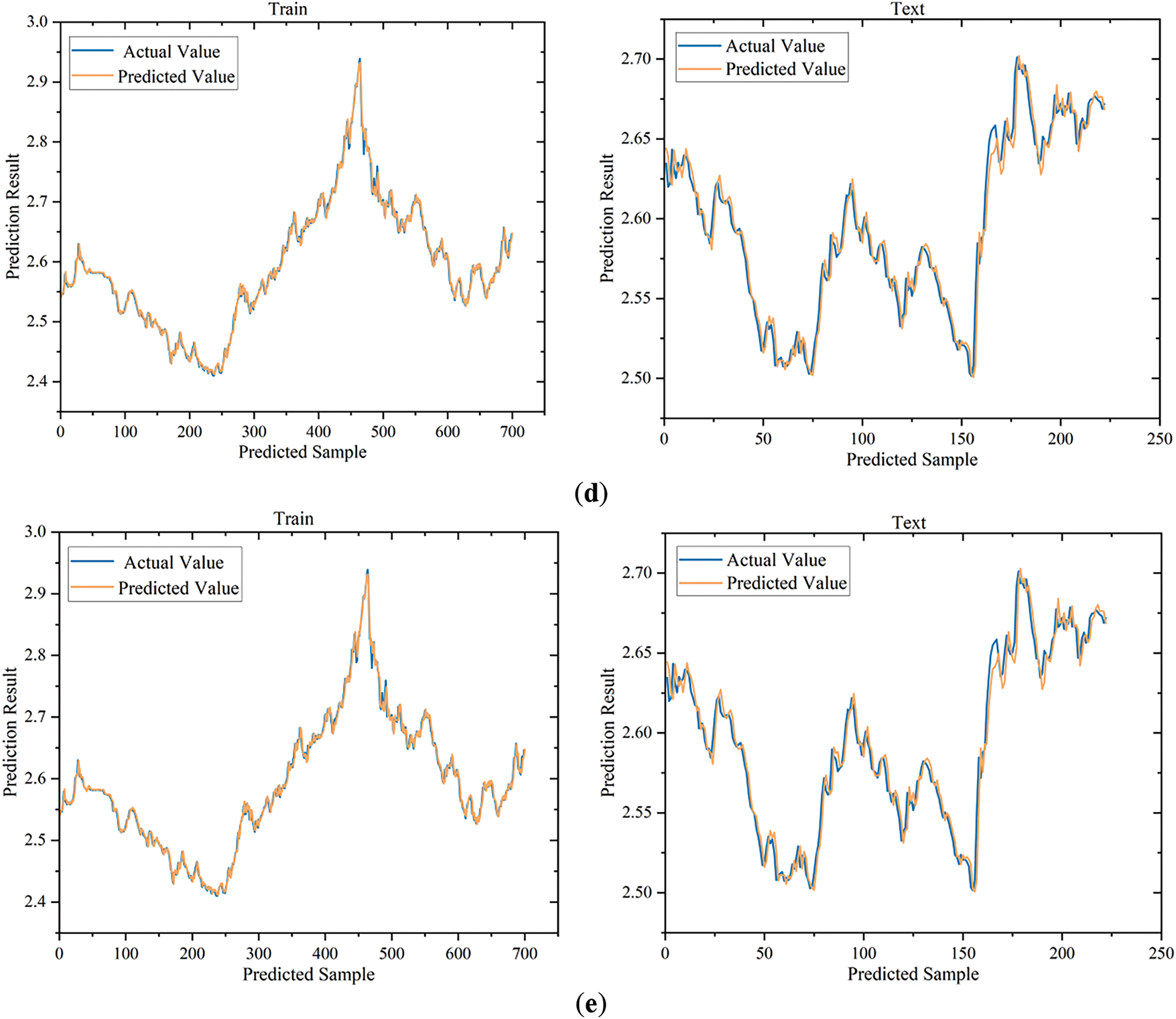
Figure 5: Comparison of the true and predicted values of each model. (a) Comparison of the true and predicted values of Transformer; (b) Comparison of the true and predicted values of LSTM-Attention; (c) Comparison of the true and predicted values of CNN-LSTM; (d) Comparison of the true and predicted values of CNN-BiLSTM-Attention; (e) Comparison of the true and predicted values of CNN-Transformer

Figure 6: Comparison diagram of each model index
A smaller Root Mean Square Error (RMSE) value means the model’s predictive accuracy is higher. The formula for the Root Mean Square Error is as follows:
where
The smaller the Mean Absolute Error (MAE) value, the closer the forecasting model’s predictions are to the true values, indicating higher forecasting accuracy. The formula for the Mean Absolute Error is as follows:
The closer the value of the Coefficient of Determination (R2) is to 1, the better the model fits the data. The formula for the Coefficient of Determination is as follows:
where
This paper compares the Transformer, LSTM-attention, CNN-LSTM, CNN-BiLSTM-Attention and CNN-Transformer models, as shown in Table 2. The experimental results indicate that the CNN-Transformer model performs best in terms of predictive accuracy, with the lowest RMSE and MAE values of 0.0063 and 0.00421, respectively, indicating the smallest prediction error. At the same time, the CNN-Transformer model’s R2 value is closest to 1, reaching 0.99635, demonstrating the strongest data explanatory power. Following that is the CNN-BiLSTM-Attention model, with RMSE and MAE values of 0.00718 and 0.00512, respectively, and an R2 value of 0.99543. The Transformer model performs relatively weaker in these three metrics, with RMSE and MAE values of 0.00705 and 0.00559, respectively, and an R2 value of 0.99425. Considering these evaluation metrics, the CNN-Transformer model has the best overall performance on the test set, indicating that it is superior to the other two models in both predictive accuracy and model interpretability.

As shown in Table 3, the CNN-Transformer model performs best in terms of prediction accuracy, with the lowest RMSE and MAE values of 0.009 and 0.00673, respectively, indicating the smallest prediction error. At the same time, the CNN-Transformer model has the highest R2 value, reaching 0.97233, demonstrating the strongest data explanatory power. Following closely is the CNN-LSTM model, with RMSE and MAE values of 0.00952 and 0.00711, respectively, and an R2 value of 0.96906. The LSTM-attention model performs relatively weaker in these three metrics, with RMSE and MAE values of 0.01168 and 0.00847, respectively, and an R2 value of 0.95336. Considering these evaluation metrics, the CNN-Transformer model has the best overall performance on the test set, indicating that it is superior to the other two models in both predictive accuracy and model interpretability.

4.2 Analysis of Algorithm Fitness before and after Improvement
To verify the performance of the improved Zebra Optimization Algorithm (IZOA), IZOA is compared with the ZOA and PSO (Particle Swarm Optimization) intelligent optimization algorithms, using the worst value, best value, average value, and standard deviation as comparative data [20]. The worst and best values reflect the stability of the algorithm, the average value demonstrates the precision of the algorithm, and the standard deviation shows the robustness of the algorithm.
As can be seen from Table 4, the IZOA algorithm demonstrated the best optimal values and stability in most cases, indicating its significant advantage in the optimization problems of these specific functions. Specifically, IZOA found the optimal solutions for functions f1 and f6, and its standard deviation was zero, which means its performance on these functions was very stable. The PSO algorithm performed best on function f3, while the ZOA algorithm excelled on function f2. Furthermore, the average values and standard deviations of the IZOA algorithm in most cases were much smaller than those of PSO and ZOA, indicating its potential superiority in global search capability and stability.

To better showcase the performance of the improved algorithm, as well as its convergence speed and precision, the performance of the three algorithms on six test functions is presented in the form of convergence curves, as shown in Fig. 7. It is evident that the improved algorithm outperforms other optimization algorithms in optimization capability.

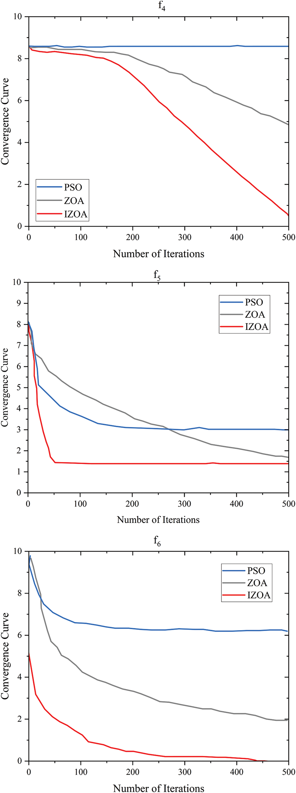
Figure 7: Convergence plot of each algorithm
4.3 Economic and Stability Analysis
As shown in Fig. 8, the system has achieved remarkable results in total cost control. Comparing Scenario 1, Scenario 2, and the method proposed in this paper, their costs are 4160 yuan, 3200 yuan, and 2890 yuan, respectively. It can be seen that the scheme proposed in this paper can effectively reduce operational costs. As shown in Fig. 9, the system stability is superior. Comparing Scenario 1, Scenario 2, and the method proposed in this paper, their simplified L-indices are 0.242, 0.189, and 0.156, respectively. It can be seen that the scheme proposed in this paper can effectively improve the stability of the system.
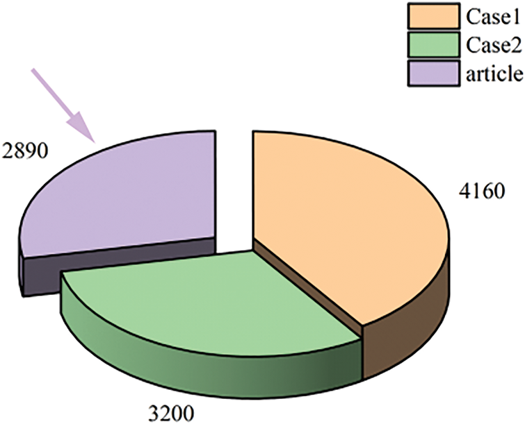
Figure 8: Economic comparison diagram

Figure 9: Stability comparison diagram
With the high proportion of new energy integration, the stability of power systems faces new challenges. To meet this challenge, this paper proposes a power stability system based on large language models, aiming to improve the safety and stability of power systems through advanced deep learning technology. Based on the research in this paper, we draw the following conclusions:
This paper constructs a CNN-Transformer prediction model for fault diagnosis in microgrids. The model processes the data by combining the local feature extraction capability of Convolutional Neural Networks (CNN) and the global dependency modeling capability of the Transformer model, showing great potential in power safety diagnosis. The experimental results indicate that the CNN-Transformer model demonstrated outstanding predictive performance in microgrid fault diagnosis. On the training set, the model achieved a root mean square error (RMSE) of 0.0063, a mean absolute error (MAE) of 0.00421, and a coefficient of determination (R2) of 0.99635, indicating the smallest prediction error and the strongest data interpretability. On the test set, the RMSE was 0.009, the MAE was 0.00673, and the R2 was 0.97233, also showing the advantage of predictive accuracy.
This paper takes the system’s economy and stability as the objective functions and uses the improved Zebra Algorithm for solving. By comparing the operating costs under different scenarios, the approach proposed in this paper can effectively reduce costs. Specifically, the cost for Scenario 1 is 4160 yuan, for Scenario 2 it is 3200 yuan, and the cost for the method presented in this paper is 2890 yuan, demonstrating the effect of cost reduction. In terms of system stability, the solution proposed in this paper also performs well. The simplified L-index for Scenario 1 is 0.242, for Scenario 2 it is 0.189, and for the method in this paper, the simplified L-index is 0.156, indicating a significant improvement in system stability.
This paper uses the improved Zebra Algorithm for solving, and the improved algorithm significantly enhances the adaptability and robustness of the algorithm by introducing an elite chaotic reverse learning strategy to increase the probability of selecting better solutions. This paper compares the improved Zebra Algorithm with other algorithms, using the worst value, best value, average value, and standard deviation as comparative data, to verify its advantages in optimization problems.
Acknowledgement: The authors would like to express their sincere gratitude for the support and sponsorship provided by Huai’an Hongneng Group Co., Ltd. in the research and development of the “Research on Power Safety Auxiliary Decision System Based on Large Language Models” project. This project under the Science and Technology Project Contract has significantly benefited from the insights and resources contributed by the company.
Funding Statement: The research project, “Research on Power Safety Assisted Decision System Based on Large Language Models” (Project Number: JSDL24051414020001), acknowledges with gratitude the financial and logistical support it has received. This study would not have been possible without the generous backing provided by the project sponsors.
Author Contributions: Study conception and design: Lei Shen, Chutong Zhang, Jie Ji; data collection: Yuwei Ge, Shanyun Gu; analysis and interpretation of results: Qiang Gao, Wei Li; draft manuscript preparation: Chutong Zhang. All authors reviewed the results and approved the final version of the manuscript.
Availability of Data and Materials: The data that support the findings of this study are available from the corresponding author, Jie Ji, upon reasonable request.
Ethics Approval: Not applicable.
Conflicts of Interest: The authors declare no conflicts of interest to report regarding the present study.
References
1. Liu Y, Peng M, Gao X. Dynamic vulnerability assessment of hybrid system considering wind power uncertainty. Energy Rep. 2024;11:3721–30. doi:10.1016/j.egyr.2024.03.033. [Google Scholar] [CrossRef]
2. Eskandari A, Nedaei A, Milimonfared J, Aghaei M. A multilayer integrative approach for diagnosis, classification and severity detection of electrical faults in photovoltaic arrays. Expert Syst Appl. 2024;252(14):124111. doi:10.1016/j.eswa.2024.124111. [Google Scholar] [CrossRef]
3. Ajagekar A, You F. Quantum computing based hybrid deep learning for fault diagnosis in electrical power systems. Appl Energy. 2021;303(6):117628. doi:10.1016/j.apenergy.2021.117628. [Google Scholar] [CrossRef]
4. Hao J, Zhan H, Xiao C, Pei H, Wang L. A method of operation status evaluation and fault diagnosis for PV arrays in the scenario of digitalization. Energy Rep. 2024;12(7):3020–33. doi:10.1016/j.egyr.2024.08.071. [Google Scholar] [CrossRef]
5. Liu B, Chen S, Gao L. Combining residual convolutional LSTM with attention mechanisms for spatiotemporal forest cover prediction. Environ Model Softw. 2025;183(4):106260. doi:10.1016/j.envsoft.2024.106260. [Google Scholar] [CrossRef]
6. Bharatheedasan K, Maity T, Kumaraswamidhas LA, Durairaj M. Enhanced fault diagnosis and remaining useful life prediction of rolling bearings using a hybrid multilayer perceptron and LSTM network model. Alex Eng J. 2025;115(8):355–69. doi:10.1016/j.aej.2024.12.007. [Google Scholar] [CrossRef]
7. Hu L, Wang J, Lee HP, Wang Z, Wang Y. Wear prediction of high performance rolling bearing based on 1D-CNN-LSTM hybrid neural network under deep learning. Heliyon. 2024;10(17):e35781. doi:10.1016/j.heliyon.2024.e35781. [Google Scholar] [PubMed] [CrossRef]
8. Lu XQ, Tian J, Liao Q, Xu ZW, Gan L. CNN-LSTM based incremental attention mechanism enabled phase-space reconstruction for chaotic time series prediction. J Electron Sci Technol. 2024;22(2):100256. doi:10.1016/j.jnlest.2024.100256. [Google Scholar] [CrossRef]
9. Zhao P, Hu W, Cao D, Zhang Z, Liao W, Chen Z, et al. Enhancing multivariate, multi-step residential load forecasting with spatiotemporal graph attention-enabled transformer. Int J Electr Power Energy Syst. 2024;160(6):110074. doi:10.1016/j.ijepes.2024.110074. [Google Scholar] [CrossRef]
10. Ibrahim Mohammad Ata K, Khair Hassan M, Ghany Ismaeel A, Abdul Rahman Al-Haddad S, Alquthami T, Alani S. A multi-Layer CNN-GRUSKIP model based on transformer for spatial−TEMPORAL traffic flow prediction. Ain Shams Eng J. 2024;15(12):103045. doi:10.1016/j.asej.2024.103045. [Google Scholar] [CrossRef]
11. Ding Y, Yi Z, Xiao J, Hu M, Guo Y, Liao Z, et al. CTH-Net: a CNN and Transformer hybrid network for skin lesion segmentation. iScience. 2024;27(4):109442. doi:10.1016/j.isci.2024.109442. [Google Scholar] [PubMed] [CrossRef]
12. Wu X, Feng Y, Xu H, Lin Z, Chen T, Li S, et al. CTransCNN: combining transformer and CNN in multilabel medical image classification. Knowl Based Syst. 2023;281(2):111030. doi:10.1016/j.knosys.2023.111030. [Google Scholar] [CrossRef]
13. Ahn JM, Kim J, Kim H, Kim K. Harmful cyanobacterial blooms forecasting based on improved CNN-transformer and temporal fusion transformer. Environ Technol Innov. 2023;32(1548):103314. doi:10.1016/j.eti.2023.103314. [Google Scholar] [CrossRef]
14. Hendria WF, Phan QT, Adzaka F, Jeong C. Combining transformer and CNN for object detection in UAV imagery. ICT Express. 2023;9(2):258–63. doi:10.1016/j.icte.2021.12.006. [Google Scholar] [CrossRef]
15. Bagherzadeh L, Kamwa I, Alharthi YZ. Hybrid strategy of flexibility regulation and economic energy management in the power system including renewable energy hubs based on coordination of transmission and distribution system operators. Energy Rep. 2024;12(23):1025–43. doi:10.1016/j.egyr.2024.06.061. [Google Scholar] [CrossRef]
16. Jia Y, Zuo T, Li Y, Bi W, Xue L, Li C. Finite-time economic model predictive control for optimal load dispatch and frequency regulation in interconnected power systems. Glob Energy Interconnect. 2023;6(3):355–62. doi:10.1016/j.gloei.2023.06.009. [Google Scholar] [CrossRef]
17. Yoon DH, Yoon J. Development of a real-time fault detection method for electric power system via transformer-based deep learning model. Int J Electr Power Energy Syst. 2024;159(4):110069. doi:10.1016/j.ijepes.2024.110069. [Google Scholar] [CrossRef]
18. Titz M, Pütz S, Witthaut D. Identifying drivers and mitigators for congestion and redispatch in the German electric power system with explainable AI. Appl Energy. 2024;356:122351. doi:10.1016/j.apenergy.2023.122351. [Google Scholar] [CrossRef]
19. Wu X, Ji Q, Liu F, Du Q, Xu W. Optimal operation strategy of power system based on stochastic risk avoidance. Results Eng. 2024;21(4):101832. doi:10.1016/j.rineng.2024.101832. [Google Scholar] [CrossRef]
20. Ji J, Zhou M, Guo R, Tang J, Su J, Huang H, et al. A electric power optimal scheduling study of hybrid energy storage system integrated load prediction technology considering ageing mechanism. Renew Energy. 2023;215(1):118985. doi:10.1016/j.renene.2023.118985. [Google Scholar] [CrossRef]
Cite This Article
 Copyright © 2025 The Author(s). Published by Tech Science Press.
This work is licensed under a Creative Commons Attribution 4.0 International License , which permits unrestricted use, distribution, and reproduction in any medium, provided the original work is properly cited.
 Downloads
 Citation Tools