
 Submit a Paper
 Propose a Special lssue
 Open Access
ARTICLE

Bilevel Planning of Distribution Networks with Distributed Generation and Energy Storage: A Case Study on the Modified IEEE 33-Bus System
State Key Laboratory of Reliability and Intelligence of Electrical Equipment, Hebei University of Technology, Tianjin, 300130, China
* Corresponding Author: Lingling Li. Email:
Energy Engineering 2025, 122(4), 1337-1358. https://doi.org/10.32604/ee.2025.060105
Received 24 October 2024; Accepted 03 February 2025; Issue published 31 March 2025
 View Full Text
 Download PDF
Abstract
Rational distribution network planning optimizes power flow distribution, reduces grid stress, enhances voltage quality, promotes renewable energy utilization, and reduces costs. This study establishes a distribution network planning model incorporating distributed wind turbines (DWT), distributed photovoltaics (DPV), and energy storage systems (ESS). K-means++ is employed to partition the distribution network based on electrical distance. Considering the spatiotemporal correlation of distributed generation (DG) outputs in the same region, a joint output model of DWT and DPV is developed using the Frank-Copula. Due to the model’s high dimensionality, multiple constraints, and mixed-integer characteristics, bilevel programming theory is utilized to structure the model. The model is solved using a mixed-integer particle swarm optimization algorithm (MIPSO) to determine the optimal location and capacity of DG and ESS integrated into the distribution network to achieve the best economic benefits and operation quality. The proposed bilevel planning method for distribution networks is validated through simulations on the modified IEEE 33-bus system. The results demonstrate significant improvements, with the proposed method reducing the annual comprehensive cost by 41.65% and 13.98%, respectively, compared to scenarios without DG and ESS or with only DG integration. Furthermore, it reduces the daily average voltage deviation by 24.35% and 10.24% and daily network losses by 55.72% and 35.71%.Keywords
The electric power industry is the largest contributor to carbon emissions, exerting a significantly impacts on climate change [1]. DWT and DPV have emerged as preferred renewable energy sources due to their pollution-free nature and widespread distribution.
As commercial models and supportive legal policies for DG continue to evolve [2], the integration of DG into distribution networks becomes increasingly critical. This is particularly relevant in the context of rising electricity costs, the shift from traditional fossil fuels, and ongoing power supply challenges caused by inadequate transmission capacity [3]. DG integration provides several benefits, including localized energy utilization, deferral of network upgrades, and adaptability to specific local conditions, thus demonstrating significant potential for modern distribution networks [4].
Despite these advantages, traditional distribution networks face persistent issues such as low terminal voltage, high line losses, and significant reactive power consumption, driven by long supply lines and rapid load changes [5]. While DG integration can enhance voltage quality, optimize reactive power flow, and improve power supply reliability, irrational planning often results in challenges such as voltage rise at connection points during peak renewable energy output and transformer overloads [6]. Furthermore, the intermittent and stochastic nature of DG exacerbates uncertainties in distribution network operations. These issues underscore the critical need for effective ESS to address the mismatch between peak DG output and load demand, smooth power output fluctuations, and reduce overall network losses [7].
Conventional methods for distribution network zoning, typically based on administrative or geographical boundaries, fail to capture electrical connectivity. Therefore, it is essential to incorporate electrical distance and power complementary characteristics during the planning stage to ensure a rational layout of DPV and ESS within the network. This approach enhances grid efficiency by mitigating local overloads and power imbalances [8].
To address DG output uncertainty, physical and statistical methods are commonly employed. Physical methods depend on weather forecasts and regional features but often yield complex and less generalizable models [9]. Statistical methods, including theoretical distribution models and kernel density estimation, have been widely used. However, these methods often depend on assumed distribution types [10], potentially leading to discrepancies between modeled and actual conditions. The Copula model, within statistical methods, offers high simulation accuracy and is suitable for diverse joint distributions, making it widely applicable in research on joint output models for wind and solar power [11]. Reference [12] proposed a methodology using multivariate Gaussian and Vine copulas to generate short-term scenarios of aggregated wind, photovoltaic, and small hydro production, evaluating their applications in reserve bidding and system scheduling. Reference [13] utilized the Frank-Copula function to generate output scenarios for wind and solar power in integrated energy systems. Case analyses indicated that scenarios simulated using this method exhibited distinct seasonal and temporal patterns, as well as correlations between wind and solar power daily outputs.
In distribution networks with numerous nodes, high DG penetration rates, small capacity, and dispersed interconnection points, the lack of unified planning during development has led to reverse overload conditions in regions with low power demand and weak supply capabilities. These overloads, occurring at specific times, severely exceed the distribution network’s capacity, primarily due to arbitrary DG and ESS siting [14]. Predetermined candidate nodes often lack validation, leading to uneconomic operational states in certain areas or periods, thereby impacting the overall efficiency of the power system. Consequently, the selection of candidate nodes during planning is crucial [15]. Reference [16] identifies candidate nodes for DG deployment based on nodes with lower cost sensitivity factors. Tests conducted on IEEE 33-bus and 69-bus systems validate the method’s effectiveness. However, the approach overlooks power-related impacts. From the perspective of improving operational reliability during planning, it is essential to enhance the complementarity and matching of power between nodes. Thus, this study opts to reflect electrical coupling relationships between nodes using electrical distance based on voltage-to-power sensitivity. In response to these challenges, this study proposes a comprehensive framework for distribution network planning that incorporates DG uncertainties, ESS integration, and power complementary characteristics to improve operational efficiency and reliability.
Distribution network planning can be approached using two main methodologies: traditional mathematical optimization techniques and artificial intelligence methods [17]. Traditional mathematical optimization typically begins with an initial solution, generated randomly or based on problem-specific characteristics within the solution space. This solution undergoes iterative updates using solving formulas until a predefined maximum number of iterations or convergence conditions are satisfied. Several models have been suggested for distribution network planning, such as the distributed robust optimization model [18], the mixed-integer quadratic constraint model [19], and the least-squares extrapolation technique [20].
In contrast to traditional mathematical optimization, based on artificial intelligence methods offer advantages in handling high-dimensional nonlinear problems inherent in distribution network planning, as they are less susceptible to local optimal [21]. Reference [22] proposed a hybrid genetic-particle swarm optimization method for optimal DG configuration. Reference [23] developed an algorithm that combines the non-dominated sorting genetic algorithm and tabu search, incorporating demand-side response for DG planning. The aforementioned studies did not incorporate ESS, limiting potential increases in DG penetration rates in distribution networks and resulting in low utilization of wind and PV power [24]. This study further develops a DG-ESS planning model that incorporates wind and solar power uncertainties with cluster partitioning, reformulated into a bilevel structure and solved using MIPSO for validation with the modified IEEE 33-bus system. The main contributions of this study are as follows:
• To address the uncertainties and correlations in wind and solar power outputs in distribution networks, a joint probability distribution model for DWT and DPV is established using the Frank-Copula function.
• To tackle the difficulty of determining the large number of DG and ESS grid-connected nodes in distribution networks, a cluster partitioning method based on electrical distance is proposed, effectively reducing the complexity of siting grid-connected nodes.
• A bilevel planning model for distribution networks incorporating DG and ESS is established, and a MIPSO algorithm adapted for mixed-integer programming is developed to efficiently solve the siting and sizing problems of DG and ESS, significantly improving the economic and operational performance of distribution networks.
The remaining sections are structured as follows: Section 2 develops models for wind and solar uncertainties, as well as a distribution network clustering model, and presents the objective functions and constraints of the planning model. Section 3 constructs a bilevel planning model for the distribution network. Section 4 conducts simulation analyses using the modified IEEE 33-bus system, comparing four different scenarios. Section 5 summarizes the research findings, conclusions, and prospects for future research.
2.1 Simulation of Wind and Solar Uncertainty
Theoretical distribution models such as the Weibull and Beta distributions are employed to analyze the probability distribution of wind and solar power output [25]. However, these models necessitate precise parameter values, which are frequently unavailable. Kernel density estimation (KDE), a non-parametric approach, calculates the probability density function by placing a kernel function around each data point and computing the weighted average of these kernels. KDE offers flexibility by not assuming a specific data distribution a priori, thus enabling better adaptation to the data’s inherent characteristics.
The KDE method assesses the influence of individual data points on the estimated value by comparing the distance between each data point and the point of interest. Data points in closer proximity to the point of interest are accorded greater weights, whereas those farther away receive diminished weights. Historical annual wind and solar power output data are organized into daily wind and solar power output samples as follows:
For a specific point
where n is the sample size, and hx is the bandwidth for WT kernel density estimation. The PV kernel density estimation is the same as Eq. (2).
The outputs of wind and solar power at a specific location display correlation alongside stochastic variability. Copula functions serve as versatile tools that connect the marginal distributions of multiple random variables to their joint distribution, effectively characterizing their correlation and dependence. In light of the observed negative correlation between wind and solar power, this study adopts the Frank Copula function to model their relationship:
where
where u =
Eq. (4) is substituted into Eq. (3) to establish the joint probability distribution function. Random sampling from this joint distribution function across each time period, followed by inverse transformation of these samples, produces comprehensive daily data on wind and solar power outputs. This approach captures both the correlation and stochastic nature inherent in these renewable energy sources. Finally, typical daily scenarios of wind and solar power outputs are generated using the K-means clustering method.
2.2 Cluster Partitioning of Distribution Networks
The partitioning of distribution network clusters is typically based on electrical distance, defined by the sensitivity relationship between voltage magnitude and injected power. The voltage magnitude-power sensitivity can be derived from the Newton-Raphson polar coordinate power flow correction equation:
Considering the distribution network is shorter in distance and has a relatively uniform load compared to the transmission network, changes in voltage magnitude are more significant than changes in voltage phase. Therefore,
In the distribution network, variations in both active and reactive power affect voltage, necessitating their inclusion in the electrical distance calculation. The coefficient Dij, which represents the overall impact of changes in the injected power at node i on the voltage magnitude at node j, is defined based on SUP and SUQ as shown in Eq. (7):
where
where n is the total number of nodes in the distribution network, and Lij represents the electrical distance between node i and node j.
After calculating the electrical distances between all nodes, clustering is conducted using the K-means algorithm. The traditional K-means algorithm randomly selects initial cluster centers, which can result in convergence to a local optimum. To address this, the K-means++ algorithm is employed, selecting high-density nodes as initial cluster centers to enhance the selection process.
For each node, M nearest neighbors are chosen. If M is too large, the algorithm may converge to a local optimum due to overly concentrated initial cluster centers from high-density nodes. Conversely, if M is too small, the initial cluster centers may lack diversity, leading to significant deviation in clustering outcomes. Experimental iterations demonstrate that an optimal selection of M enhances clustering performance.
The sum of the electrical distances between each node i and its nearest M nodes is calculated as shown in Eq. (10):
These sums are arranged in ascending order, with the top k nodes identified as high-density nodes. These nodes are selected as the initial cluster centers in the K-means++ algorithm. The objective function for K-means++ clustering is the sum of the squared electrical distances between nodes within each cluster and the central node, as shown in Eq. (10):
where m is the number of clusters in the distribution network, Nk is the number of nodes in the k-th cluster, and
2.3.1 Upper-Layer Planning Model
Annual comprehensive cost of the distribution network:
Annual operational costs:
where
where
where
Annual Equivalent Investment Costs:
where CWT, CPV and CESS are the unit capacity investment costs of WT, PV and ESS, respectively, r is the discount rate, and n1, n2 and n3 are the service lives of WT, PV, and ESS, respectively.
Costs of Interaction with the Upper-Level Grid:
where Fbuy represents the cost of purchasing electricity from the upper-level grid, and Rsell represents the revenue from selling electricity back to the upper-level grid.
where
where
Unlike the current DG generation benefits which already cover costs and with subsidies gradually phasing out, the ESS profit mechanism is not yet perfected and the price of ESS remains high. Hence, subsidies are required for ESS generation [26].
Subsidies for ESS generation are typically structured as capacity price subsidies:
where
2.3.2 Lower-Level Operation and Control Model
The objective function is the sum of the annual network loss cost and the voltage fluctuation penalty coefficient:
Annual network loss cost:
where
Annual voltage fluctuation penalty costs:
where
where
2.5.1 Maximum Node Access DG Capacity
where
2.5.2 Node Maximum Access ESS Capacity
where
2.5.3 DG Installed Penetration Constraints
where
2.5.4 Nodal Voltage Constraints
where Ui is the voltage amplitude at node i,
where
2.5.6 Branch Transmission Power Constraints
where Sl is the transmission power of branch l, and
3 Model Optimization Methods and Solutions
3.1 Establishment and Solution of the Bilevel Model
Bilevel programming offers a structured approach for tackling intricate problems by dividing them into upper and lower levels. This hierarchical framework is employed to optimize system-wide issues. Each level is characterized by its own objective functions, decision variables, and constraints. The upper and lower levels are interlinked and collaboratively iterated to achieve the optimal solution.
In this study, the upper-level model focuses on minimizing the system’s annual comprehensive cost while determining the optimal locations and capacities of DG and ESS, these optimal configurations are fed into the lower-level model. The lower-level model is designed to minimize annual network losses and penalties associated with voltage fluctuations. Fig. 1 depicts the process of establishing and solving the bilevel model for the system.
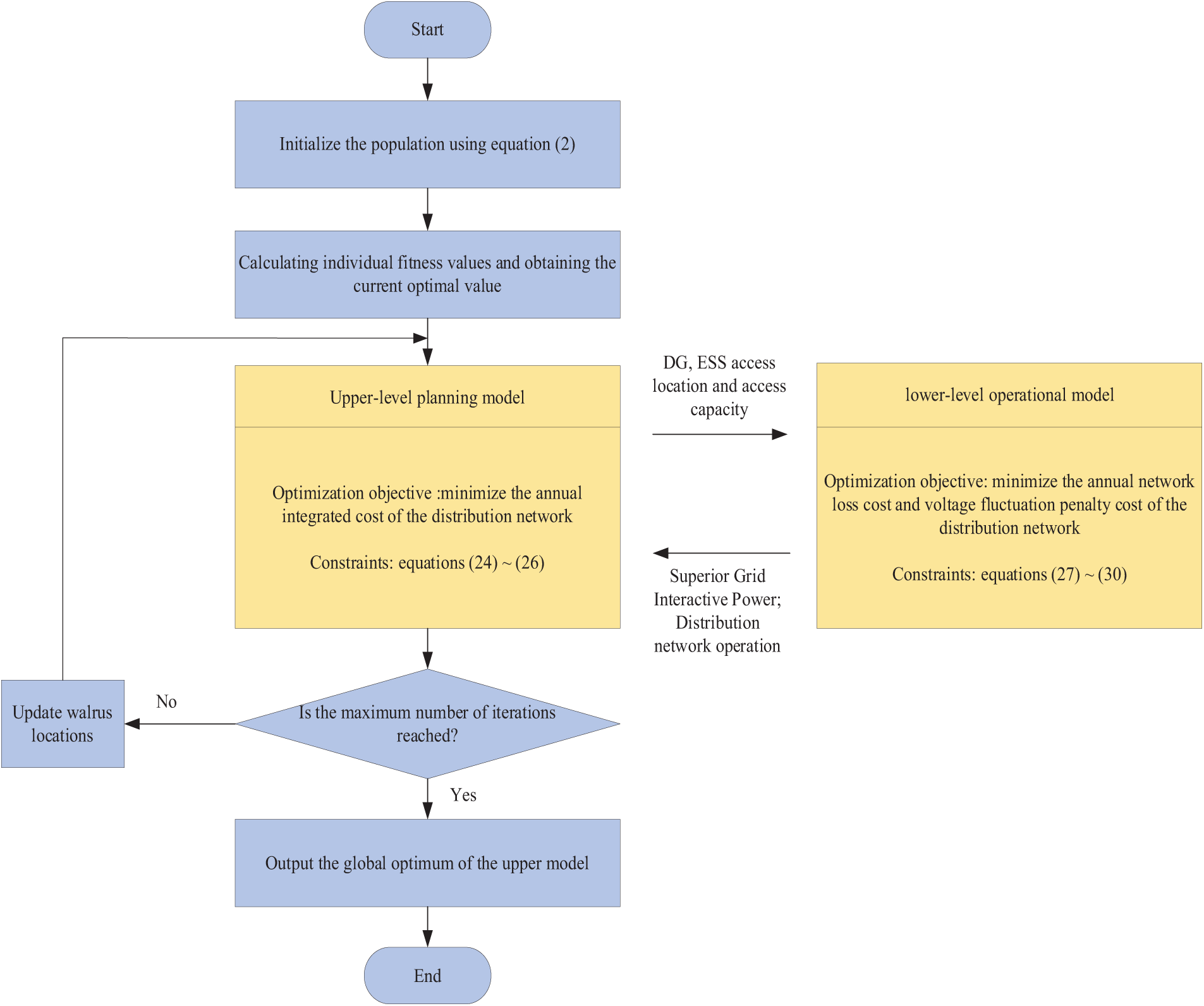
Figure 1: Distribution network two-layer planning model
The bilevel programming model links its two layers through transfer variables. The upper-level model functions as the leader, emphasizing economic benefits, while the lower-level model focuses on system operational quality. Network loss costs represent the distribution of power flows within the system, and voltage fluctuation penalty costs denote voltage variations.
The upper-level planning model first determines the decision variable x, which it then transfers to the lower-level operational model. Utilizing a second-order cone relaxation programming approach [27], the lower-level model computes the optimal power flow solution and communicates the results back to the upper-level model. These outcomes are subsequently integrated into the upper-level model’s objective function solving process. This iterative procedure continues until a global optimal solution is attained or the maximum number of iterations is reached.
Throughout the solving process, bilevel programming accounts for both the economic objectives of the upper level and the operational objectives of the lower level. The two models mutually constrain and influence each other, ultimately achieving an optimal solution that satisfies both sets of objectives. This method not only maximizes economic benefits but also ensures high system operational quality, providing substantial practical application value.
3.2 Mixed-Integer Particle Swarm Optimization Algorithm
To address the mixed-integer nonlinear characteristics of distribution network planning problems, this study introduces a MIPSO designed for mixed-integer optimization. The proposed MIPSO employs a dimension-separated update strategy to accommodate the distinct characteristics of continuous and integer variables. Decision variables are divided into continuous and integer subsets, with tailored update rules for each subset.
In mixed-integer optimization problems, integer variables must be discretized to ensure solution feasibility while maintaining the convergence properties of continuous variables. For integer variable optimization, genetic algorithm (GA) operations, including selection, crossover, and mutation, are integrated into the particle update process. In this algorithm, the decision variables of the i-th particle are defined as:
where
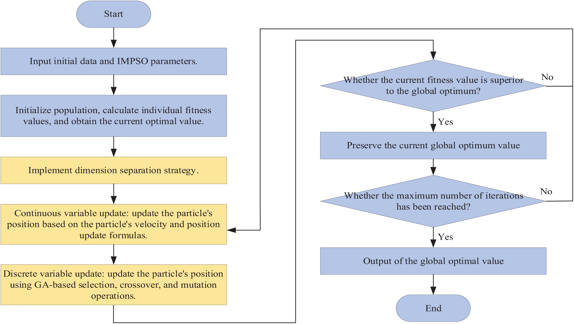
Figure 2: Mixed-integer particle swarm optimization algorithm flow chart
4.1 WT and PV Output Scenario Clustering
Data on WT and PV output from a region in North China in 2022 were utilized for this study, with per-unit values illustrated in Fig. 3. Employing the scenario generation method detailed in Section 2.1, both the WT window width hx and the PV window width hy were set to 0.05. This process yielded 1000 sets of typical daily per-unit values for wind and solar output, subsequently grouped into four distinct daily scenarios for wind and solar output using the k-means algorithm. Fig. 4 is the Frank-Copula distribution function graph for the WT and PV outputs.
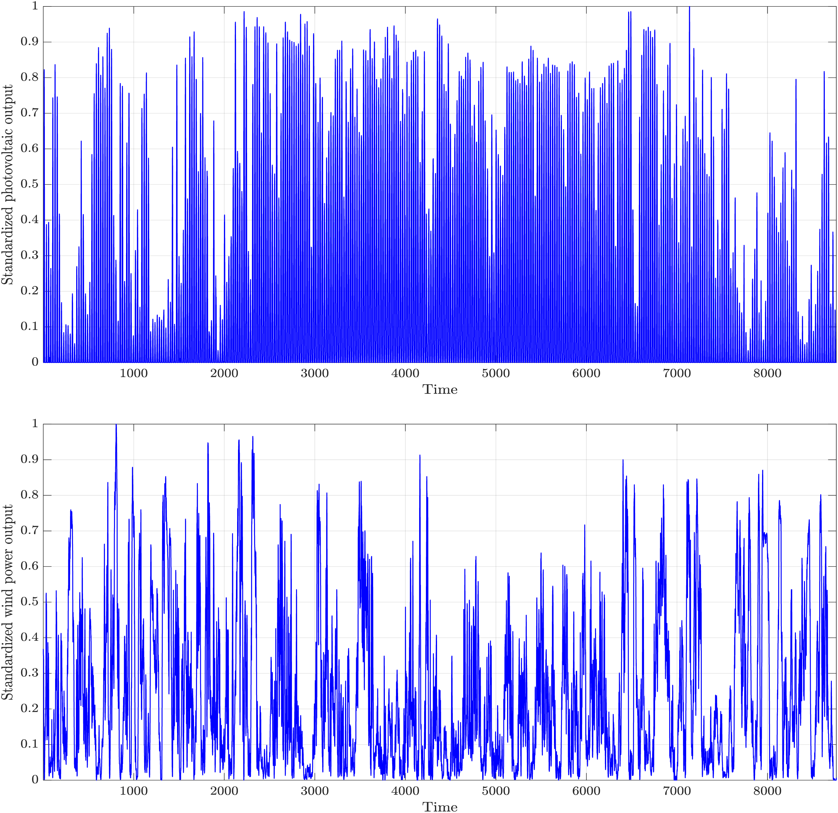
Figure 3: Historical output of PV and WT in a certain region in 2022
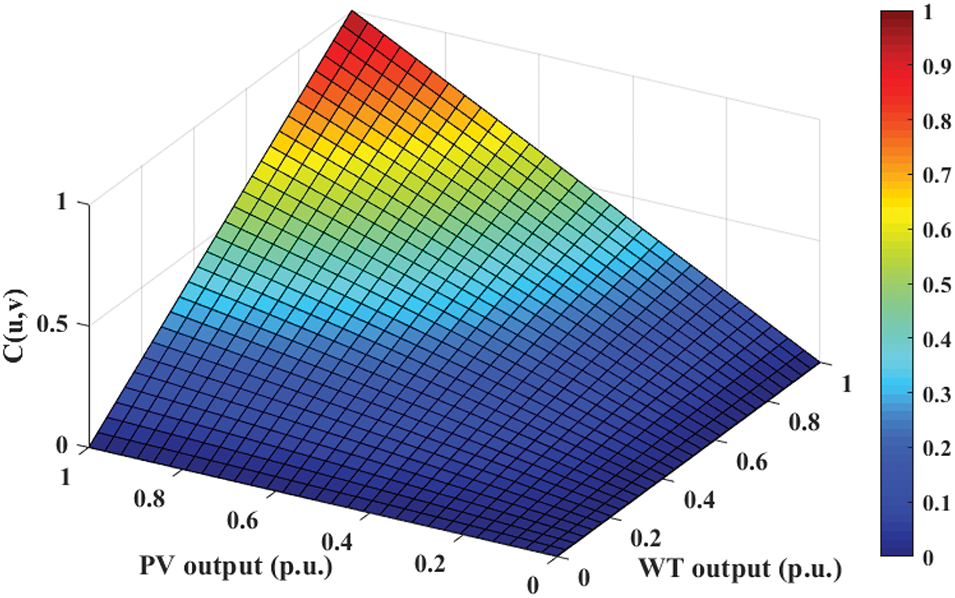
Figure 4: Frank-Copula distribution function graph
In Fig. 5, WT output appears more consistent across all scenarios. At night, as surface temperatures drop, atmospheric temperature differentials increase, fostering brisk air movement that boosts power generation, partially offsetting PV output. Within each scenario, wind and solar outputs show correlations, sometimes exhibiting consistent or opposing trends in specific periods. For instance, in Scenario 2, both wind and solar outputs decrease around noon due to intense summer heat, which stifles wind and hampers PV generation. Seasonal differences between scenarios are pronounced, reflecting distinct seasonal patterns. In Scenario 4, diminished solar irradiance during winter and earlier sunsets result in notably reduced PV output compared to other scenarios, aligning with the quarterly output trough evident in January, February, and December in Fig. 3.
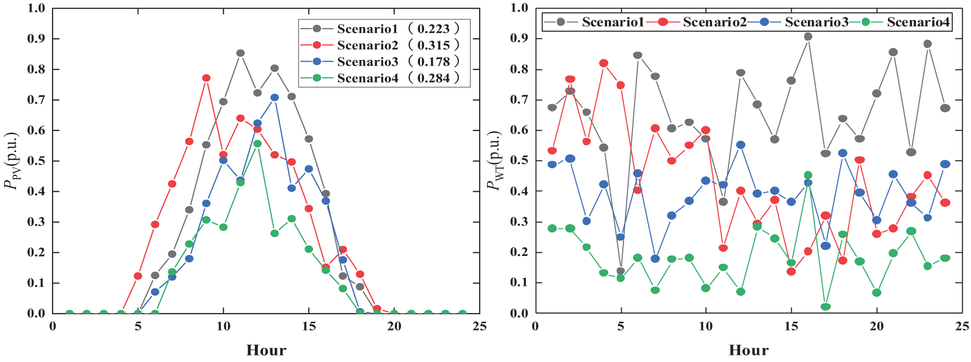
Figure 5: scenario generation results
4.2 Cluster Partitioning of IEEE 33-Bus System
The study focused on the modified IEEE 33-bus system, featuring an active load of 37.15 MW, a reactive load of 23 MW, and a system reference voltage set at 12.66 kV. Employing the K-means++ algorithm, the distribution system was segmented into clusters according to electrical distance. Fig. 6 illustrates the outcomes of cluster partitioning across various K values.
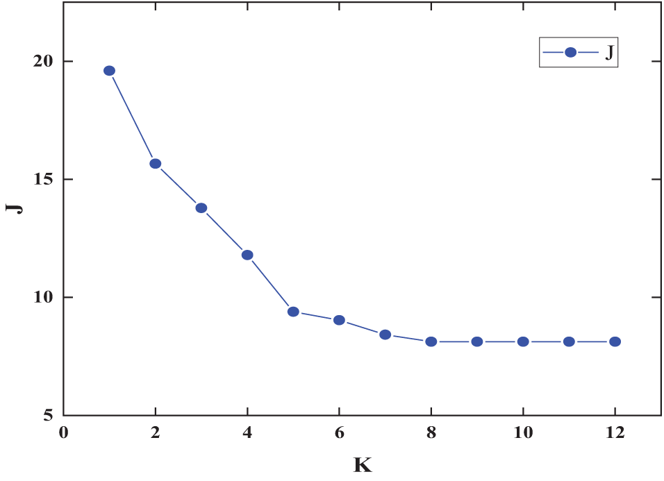
Figure 6: Partitioning indicators under different numbers of clusters
The optimal number of clusters K was determined using the elbow method [30]. Fig. 6 clearly indicates that K = 5 represents a significant inflection point. Given the structure of the distribution network, five clusters were chosen for partitioning, as illustrated in Fig. 7.
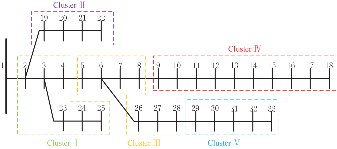
Figure 7: Distribution network division structure diagram
4.3 IEEE 33-Bus System Parameters and Optimization Settings
The system is permitted to export electricity to the main grid, with exported electricity priced at 70% of the prevailing electricity rate. Table 1 outlines additional key parameters of the system. The power distribution ratios for individual load nodes are configured using default settings, and fluctuations in system load over time are depicted in Fig. 8.
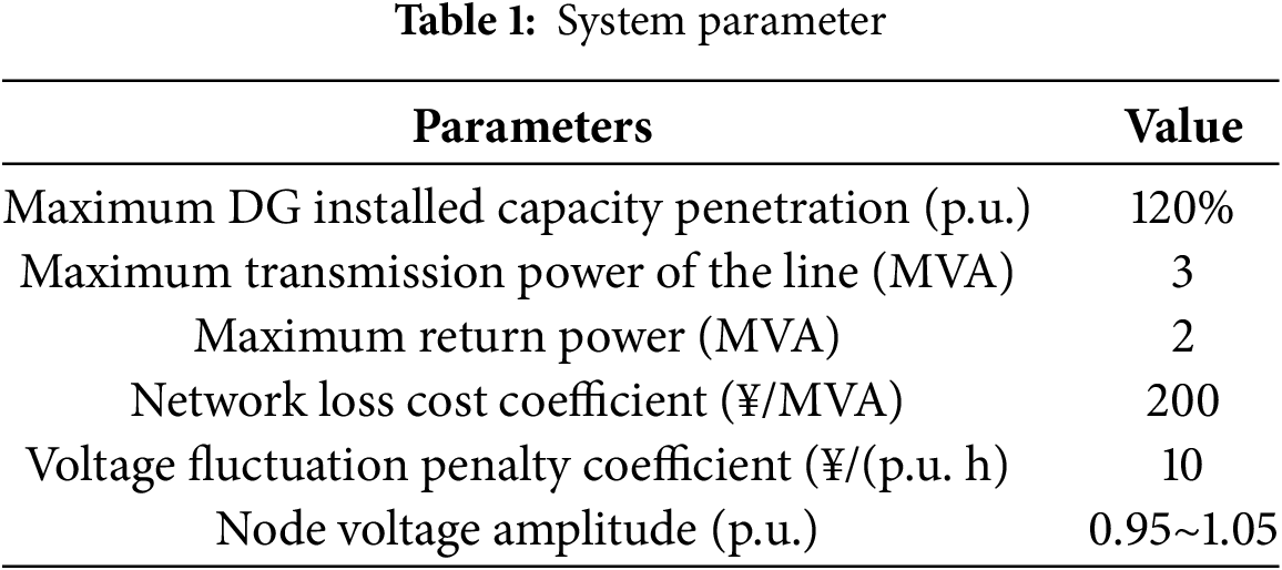
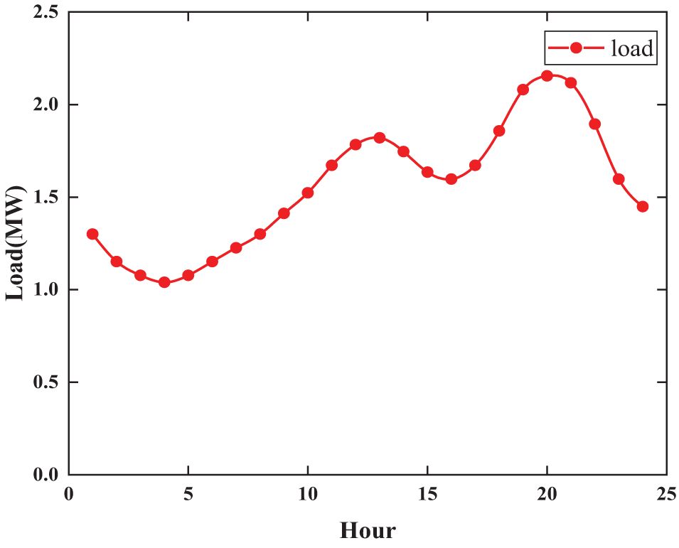
Figure 8: System daily load fluctuation diagram
The base electricity price under peak-valley tariffs is ¥560/MW. The coefficients for periods of deep valley, low valley, flat periods, high peak, and deep peak are 0.2, 0.4, 1, 1.3, and 1.8 times the base price, respectively, as depicted in Fig. 9.
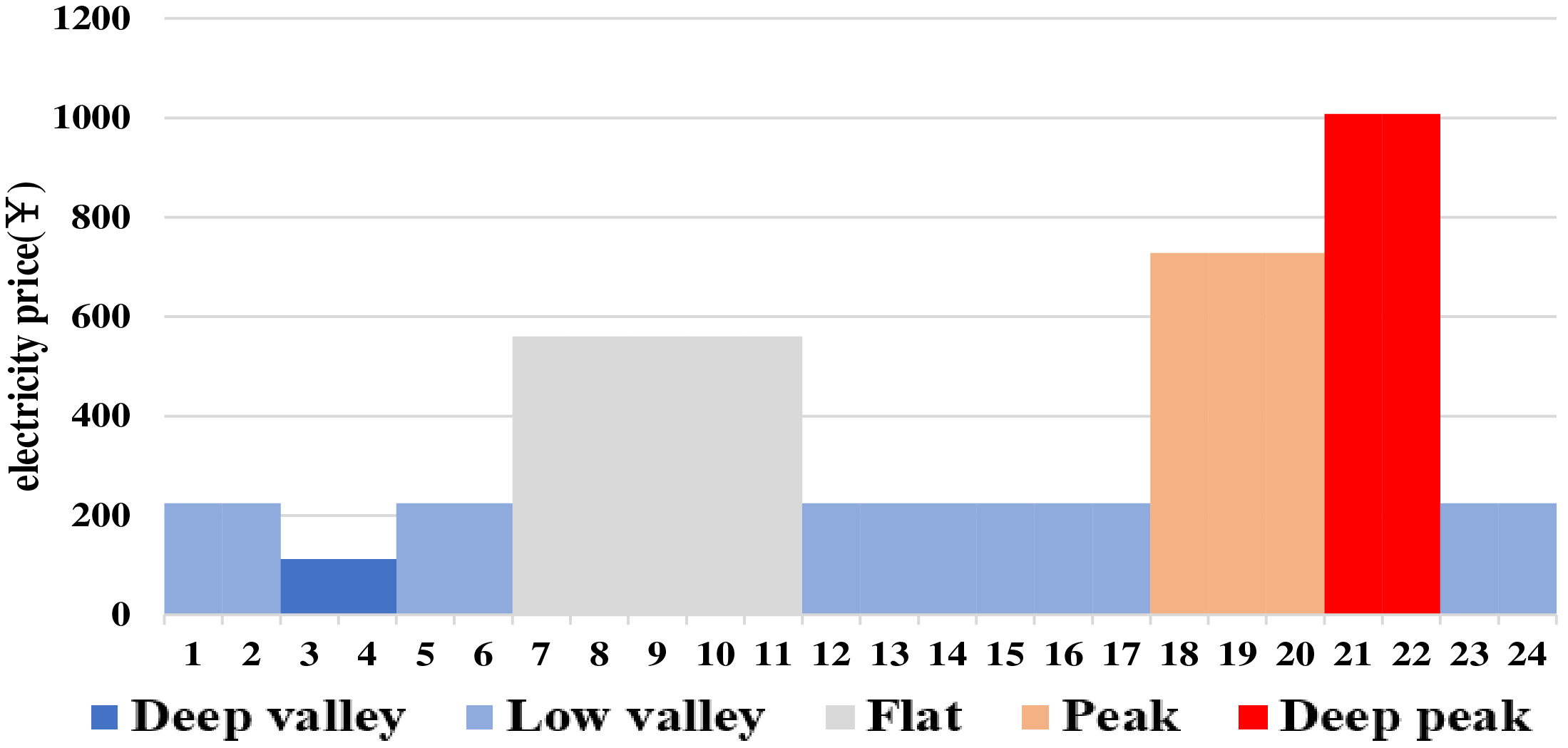
Figure 9: System daily peak and valley electricity price
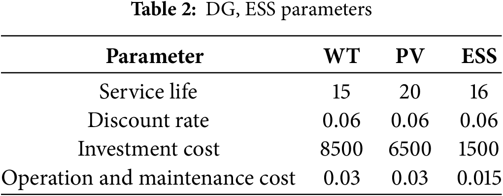
Based on the relatively short spatiotemporal distances within the distribution network in the same region, the DG output characteristics are assumed to be uniform. To minimize the lifespan reduction of the ESS caused by deep discharges and high-power charge/discharge cycles [31], the minimum ESS charge level is set at 10% of its capacity, with the charge/discharge efficiency limited to 30% of the capacity. Additionally, the compensation price for ESS capacity follows peak and off-peak electricity prices, with a base rate of ¥100/MW. The key parameters of both DG and ESS systems are detailed in Table 2.
The maximum number of iterations in the MIPSO algorithm is set to 100. For continuous variable optimization, the number of particles is set to 30, the learning parameters C1 and C2 are both 2, the maximum value of the inertia weight w is 0.9, and the minimum value is 0.1, the dimensionality is set to 15, corresponding to the capacities of DPV, DWT, and ESS in the five clusters. For integer variable optimization, the population size remains 30, the crossover probability is 0.8, and the mutation probability is 0.05, the dimensionality is also set to 15, corresponding to the locations of PV, WT, and ESS in the five clusters.
4.4 Economic Evaluation of Planning Results
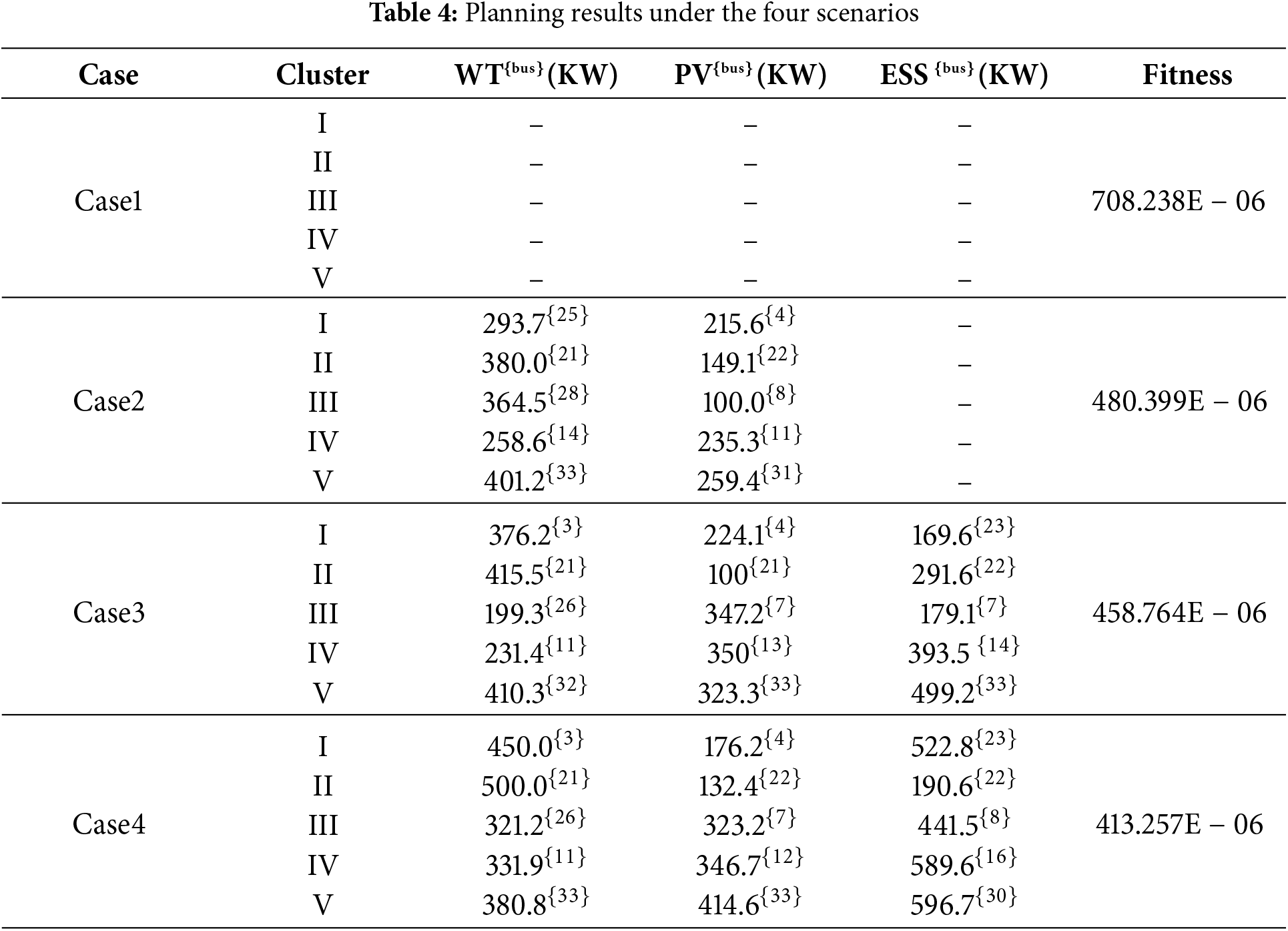
Each cluster in the model is configured to include one access point for DWT, DPV, and ESS, respectively, allowing multiple devices to connect to the same node. The access capacity for DWT and DPV at each node is limited to 100–500 kW, while ESS access is restricted to 100–700 kW. Table 3 shows the DG and ESS planning results of each cluster after MIPSO solution.
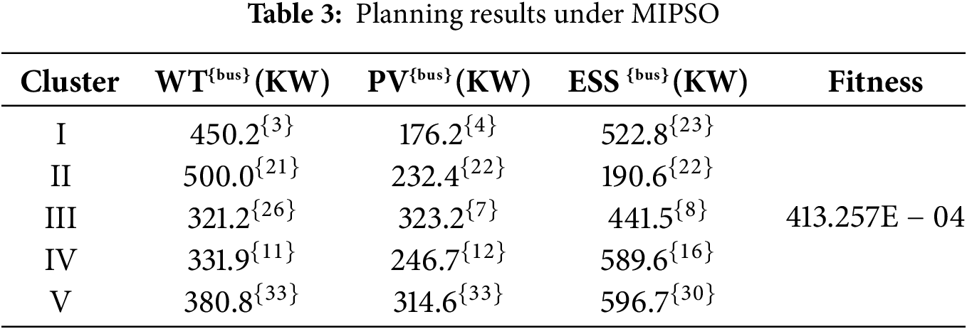
Table 3 presents planning outcomes applied to the modified IEEE 33-bus system. DWT capacities generally exceed those of DPV. This disparity arises because DWT, despite a slightly higher unit cost than DPV, offers longer daily generation durations, thereby delivering superior overall daily generation benefits.
In terms of cluster analysis, Cluster II exhibits the highest DG planning capacity, facilitated by its ability to inject electricity back into the upstream grid, thereby reducing network losses compared to other clusters. Within clusters, DG capacity correlates positively with ESS capacity. This relationship emerges because surplus DG generation within clusters tends to be absorbed internally by the system. The topology diagram of the planning results in Table 3 is shown in Fig. 10.
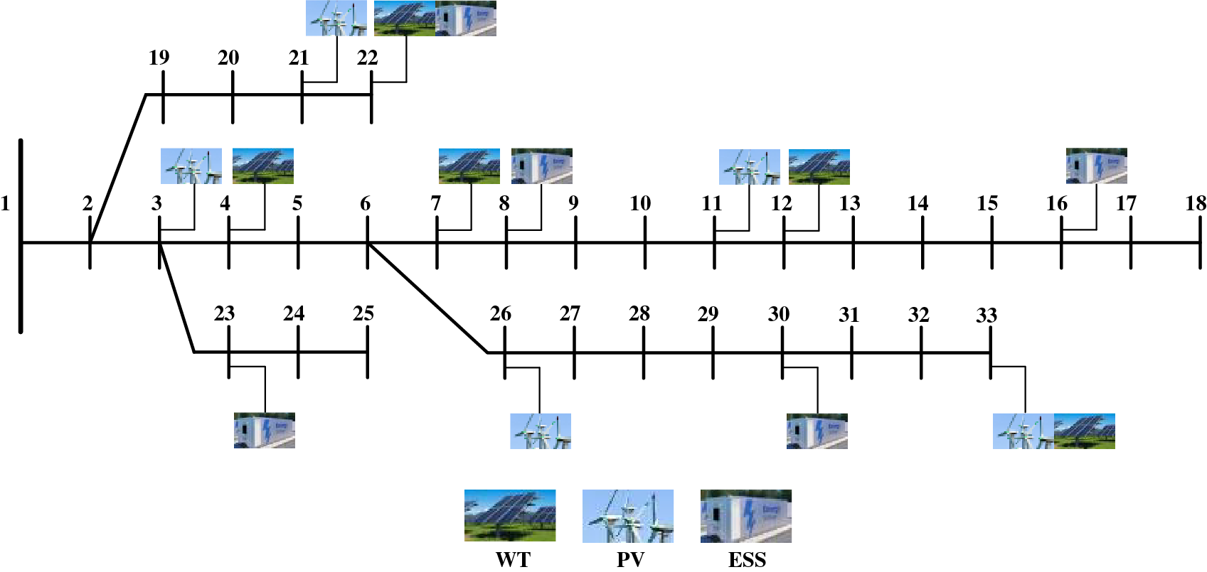
Figure 10: Modified IEEE 33-bus system DG-ESS planning diagram under MIPSO
The operational performance of the modified IEEE 33-bus distribution network is assessed based on economic benefits and power quality considerations. Four scenarios are examined to validate the efficacy of the proposed model:
Case1: No installation of DG or ESS.
Case2: Installation of DG using the algorithm and model proposed herein, without ESS.
Case3: Installation of DG and ESS using the algorithm and model proposed herein, without accounting for the compensation price for energy storage capacity.
Case 4: Installation of DG and ESS using the algorithm and model proposed herein, accounting for the compensation price for energy storage capacity.
Table 4 demonstrates that deploying DG effectively reduces the operational costs of the distribution network. In Case2, annual comprehensive costs decrease by 32.17% compared to Case1, with DG benefits covering its construction costs, indicating substantial economic gains. This reduction is attributed to declining DG unit prices over recent decades due to technological advancements. In Case4, compared to Case1, annual comprehensive costs decrease by 41.65%, indicating that the combined integration of DG and ESS achieves higher economic benefits than the sole integration of DG. In Case3, annual comprehensive costs decrease by 4.50% compared to Case2, primarily because ESS are relatively new, with their unit prices still requiring further market development. Presently, profitability from energy storage based solely on peak-valley arbitrage barely offsets costs. In Case4, annual comprehensive costs decrease by 9.92% compared to Case3, attributed to subsidies for energy storage capacity prices. Additionally, introducing energy storage capacity pricing increases energy storage penetration rates by 52.72%.
4.5 Operational Quality Analysis of Planning Results
The operational quality analysis of the distribution network in this study focuses on power quality and network loss levels. Fig. 11 illustrates the three-dimensional voltage distribution on a typical summer day across the four scenarios. Table 5 details daily voltage deviations and network losses for these scenarios.
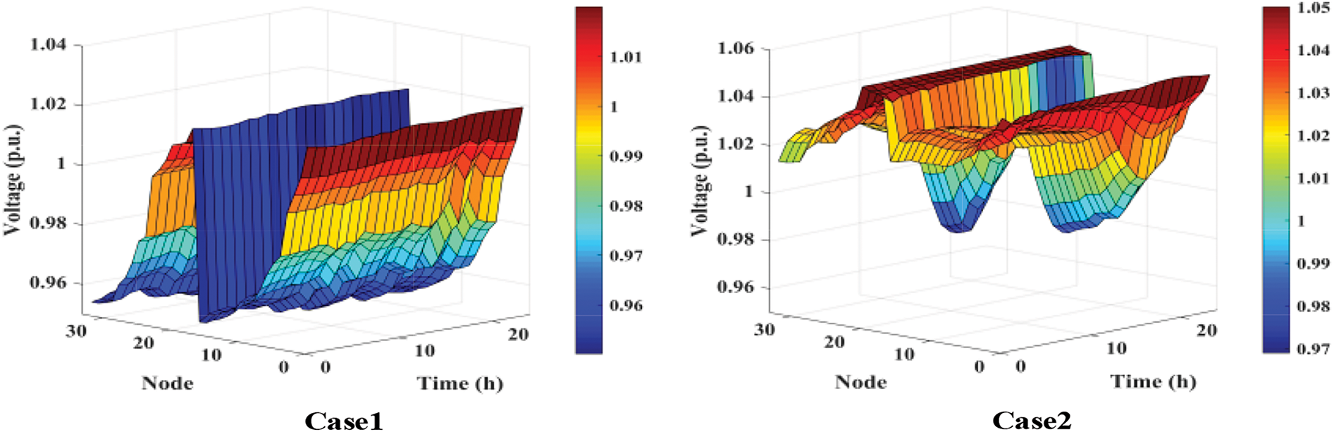
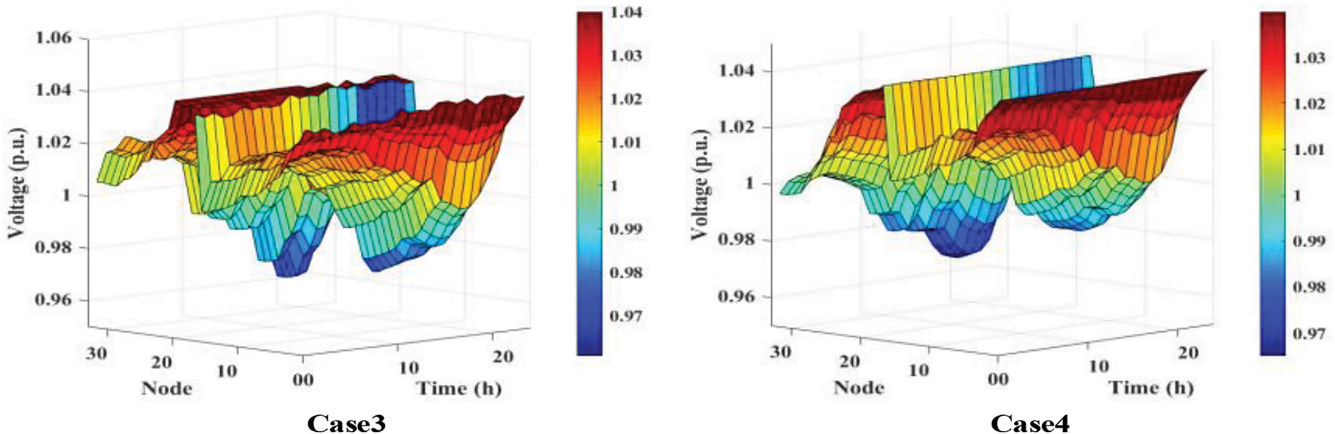
Figure 11: Typical summer daily voltage distribution under four cases
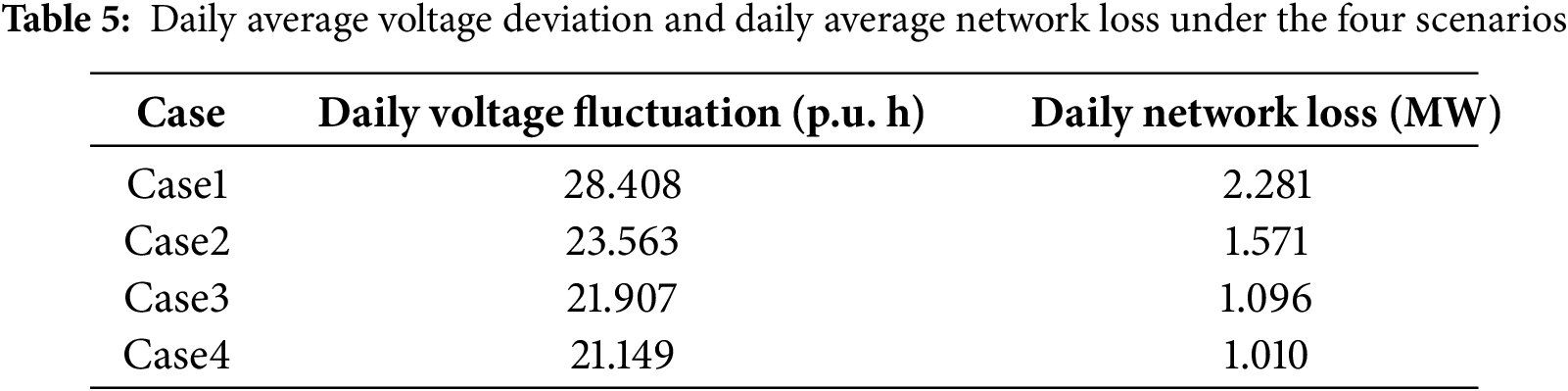
Fig. 11 illustrates that in Case1, without DG and ESS, there are notable voltage fluctuations across distribution network nodes. Only nodes close to the upstream main grid maintain voltage around 1.00 p.u., while most end nodes experience low voltage. In Case2, introducing DG resolves low voltage issues at end nodes, yet excessive DG causes overvoltage at installation sites and nearby nodes. Case3 shows that installing DG and ESS concurrently effectively mitigates DG-induced overvoltage, resulting in smoother voltage fluctuations across the network. In Case4, with higher DG and ESS penetration than Case3, overall voltage fluctuation reduction is modest, but localized areas experience more pronounced voltage stabilization.
Table 5 illustrates that Case2 exhibits a 17.06% reduction in daily voltage deviation compared to Case1, accompanied by a 31.13% decrease in network losses. This installation of DG effectively enhances node voltage and optimizes internal power flow within the distribution network. In Case3, voltage values range from approximately 0.96 to 1.04 p.u., indicating improved node power supply quality. In Case4, the daily voltage deviation and network losses are the lowest, with reductions of 24.35% and 55.72%, respectively, compared to Case1. This highlights that appropriate ESS subsidies promote energy storage market growth and larger ESS capacities effectively mitigate voltage fluctuations and reduce power company losses due to network inefficiencies.
In response to escalating climate change from excessive carbon emissions, integrating DG and ESS into the grid at large scales and high capacities has become inevitable. This study aims to determine optimal locations and capacities for DG and ESS grid integration, maximizing benefits within distribution networks. A dual-layer planning model is developed, incorporating DWT, DPV joint output, and network clustering. The MIPSO algorithm, which exhibits strong adaptability, is proposed to solve the model’s mixed-integer nonlinear characteristics. Test results demonstrate that the proposed method effectively addresses the planning challenge of DG-ESS grid integration, yielding significant improvements in both economic and operational aspects of the system. The results of the study are summarized as follows:
• A joint probability distribution model for DWT and DPV is established using the Frank-Copula function, considering the uncertainty and coupling characteristics of wind and solar power output in the distribution network.
• A cluster partitioning method based on electrical distance is developed to address the challenge of determining the number of DG and ESS interconnection nodes, significantly reducing the complexity of node selection.
• Case studies on the modified IEEE 33-bus system showed that integrating DG and ESS reduced annual comprehensive costs by 41.65%. Operationally, it mitigated voltage fluctuations by 24.35% and network losses by 55.72% daily, with energy storage subsidies increasing ESS penetration by 52.72%.
Given the continual rise in distribution network loads, strategic planning of DG-ESS within distribution networks is pivotal for their evolution and the integration of renewable energy sources. This study proposes effective solutions and strategies for determining optimal grid connection points and capacities for DG and ESS. However, opportunities for enhancement remain. Future research could concentrate on developing more sophisticated ESS models and scheduling strategies to optimize ESS longevity and profitability. Additionally, improving methods for addressing network losses, voltage fluctuations, and incorporating reactive power compensation methods are areas that warrant further investigation.
Acknowledgement: We thank our collaborators, anonymous reviewers, and the staff of the Energy Engineering journal for their contributions, feedback, and support, respectively. Special thanks go to the State Key Laboratory of Reliability and Intelligence of Electrical Equipment, Hebei University of Technology, for pivotal insights and essential resources.
Funding Statement: This research was funded by “Chunhui Program” Collaborative Scientific Research Project of the Ministry of Education of the People’s Republic of China (Project No. HZKY20220242) and the S&T Program of Hebei (Project No. 225676163GH).
Author Contributions: The authors confirm contribution to the paper as follows: study conception and design: Haoyuan Li, Lingling Li; data collection: Haoyuan Li, Lingling Li; analysis and interpretation of results: Haoyuan Li, Lingling Li; draft manuscript preparation: Haoyuan Li, Lingling Li. All authors reviewed the results and approved the final version of the manuscript.
Availability of Data and Materials: Data supporting this study are included within the article.
Ethics Approval: Not applicable.
Conflicts of Interest: The authors declare no conflicts of interest to report regarding the present study.
Nomenclature
| hx | Bandwidth for wind power kernel density estimation |
| Parameter of the Copula that controls the strength of the correlation | |
| Sup | Voltage magnitude-active power sensitivity matrix |
| SUQ | Voltage magnitude-reactive power sensitivity matrix |
| Dij | Overall impact of changes in the injected power at node i on the voltage magnitude at node j |
| Lij | Electrical distance between node i and node j |
| Nk | Number of nodes in the k-th cluster |
| Fupp | Annual comprehensive cost of the distribution network, ¥ |
| Fop | Annual operational costs, ¥ |
| Operating costs of wind power, ¥/kW | |
| Operating costs of PV power, ¥/kW | |
| Actual outputs of wind power at time t under scenario s, kW | |
| Actual outputs of PV power at time t under scenario s, kW | |
| Ms | Number of typical scenarios divided into one year |
| Probability of the scenario in one year | |
| Operating cost of energy storage, ¥/kW | |
| CWT | Unit capacity investment costs of WT, ¥/kVA |
| CPV | Unit capacity investment costs of PV, ¥/kVA |
| CESS | Unit capacity investment costs of ESS, ¥/kVA |
| Fbuy | Cost of purchasing electricity from the upper-level grid, ¥/kW |
| Rsell | Revenue from selling electricity back to the upper-level grid, ¥/kW |
| Grid electricity price at time t, ¥/kW | |
| Et, sub | Capacity price at time t, ¥/kW |
| Network loss discounting cost coefficient, ¥/kW | |
| System network loss power at moment t under scenario s, kW | |
| Voltage fluctuation penalty factor, ¥/kW | |
| Vs, t, i | Voltage amplitude at node i at moment t under scene s |
| Capacity of node i to access the DG, kW | |
| Capacity of node i to access the DG, kW | |
| Pk, DG | Planning capacity of DG in k clusters, kW |
| Pload | Total system load, kW |
| Ui | Voltage amplitude at node i |
| PESS, k | Maximum charging and discharging power of the ESS in cluster k, kW |
| Charging and discharging efficiency of ESS | |
| ue,k,t | Charging and discharging flag of the ESS |
| SOCk,t | State of charge of the ESS in cluster k at time t |
| Sk,0 | Initial state of charge of the ESS in cluster k |
References
1. Pavel T, Polina S. Heterogeneity of the impact of energy production and consumption on national greenhouse gas emissions. J Clean Prod. 2024;434(3):139638. doi:10.1016/j.jclepro.2023.139638. [Google Scholar] [CrossRef]
2. Lind L, Chaves-Ávila JP, Valarezo O, Sanjab A, Olmos L. Baseline methods for distributed flexibility in power systems considering resource, market, and product characteristics. Utilit Policy. 2024;86:101688. doi:10.1016/j.jup.2023.101688. [Google Scholar] [CrossRef]
3. Sonnsjö H. What we talk about when we talk about electricity: a thematic analysis of recent political debates on Swedish electricity supply. Ener Poli. 2024;187:114053. doi:10.1016/j.enpol.2024.114053. [Google Scholar] [CrossRef]
4. Shahbazi A, Aghaei J, Pirouzi S, Niknam T, Shafie-khah M, Catalão JPS. Effects of resilience-oriented design on distribution networks operation planning. Elect Power Syst Res. 2021;191(1):106902. doi:10.1016/j.epsr.2020.106902. [Google Scholar] [CrossRef]
5. Paul S, Poudyal A, Poudel S, Dubey A, Wang Z. Resilience assessment and planning in power distribution systems: past and future considerations. Renew Sustain Energ Rev. 2024;189(10):113991. doi:10.1016/j.rser.2023.113991. [Google Scholar] [CrossRef]
6. Ceylan O, Paudyal S, Pisica I. Nodal sensitivity-based smart inverter control for voltage regulation in distribution feeder. IEEE J Photovolt. 2021;11(4):1105–13. doi:10.1109/JPHOTOV.2021.3070416. [Google Scholar] [CrossRef]
7. Venkateswaran VB, Saini DK, Sharma M. Approaches for optimal planning of energy storage units in distribution network and their impacts on system resiliency. CSEE J Power Energy Syst. 2020;6(4):816–33. [Google Scholar]
8. Cotilla-Sanchez E, Hines PDH, Barrows C, Blumsack S, Patel M. Multi-attribute partitioning of power networks based on electrical distance. IEEE Trans Power Syst. 2013;28(4):4979–87. doi:10.1109/TPWRS.2013.2263886. [Google Scholar] [CrossRef]
9. Alkhayat G, Mehmood R. A review and taxonomy of wind and solar energy forecasting methods based on deep learning. Energy AI. 2021;4(7):100060. doi:10.1016/j.egyai.2021.100060. [Google Scholar] [CrossRef]
10. Ben Ammar R, Ben Ammar M, Oualha A. Photovoltaic power forecast using empirical models and artificial intelligence approaches for water pumping systems. Renew Energy. 2020;153(5):1016–28. doi:10.1016/j.renene.2020.02.065. [Google Scholar] [CrossRef]
11. Carvalho JH, Schwartz UB, Borges CLT. Copula based model for representation of hybrid power plants in non-sequential Monte Carlo reliability evaluation. Sustain Ener, Grids Netw. 2023;35(14):101077. doi:10.1016/j.segan.2023.101077. [Google Scholar] [CrossRef]
12. Camal S, Teng F, Michiorri A, Kariniotakis G, Badesa L. Scenario generation of aggregated Wind, Photovoltaics and small Hydro production for power systems applications. Appl Energy. 2019;242(3):1396–406. doi:10.1016/j.apenergy.2019.03.112. [Google Scholar] [CrossRef]
13. Lin S, Liu C, Shen Y, Li F, Li D, Fu Y. Stochastic planning of integrated energy system via frank-copula function and scenario reduction. IEEE Transact Smart Grid. 2022 Jan;13(1):202–12. doi:10.1109/TSG.2021.3119939. [Google Scholar] [CrossRef]
14. Valencia A, Hincapie RA, Gallego RA. Optimal location, selection, and operation of battery energy storage systems and renewable distributed generation in medium-low voltage distribution networks. J Energy Storage. 2021;34(1):102158. doi:10.1016/j.est.2020.102158. [Google Scholar] [CrossRef]
15. Bozorgavari SA, Aghaei J, Pirouzi S, Nikoobakht A, Farahmand H, Korpås M. Robust planning of distributed battery energy storage systems in flexible smart distribution networks: a comprehensive study. Renew Sustain Energ Rev. 2020;123(2):109739. doi:10.1016/j.rser.2020.109739. [Google Scholar] [CrossRef]
16. Pemmada S, Patne NR, Ajay Kumar T, Manchalwar AD. Optimal planning of power distribution network by a novel modified jaya algorithm in multiobjective perspective. IEEE Syst J. 2022;16(3):4411–22. doi:10.1109/JSYST.2021.3132300. [Google Scholar] [CrossRef]
17. Rastgou A. Distribution network expansion planning: an updated review of current methods and new challenges. Renew Sustain Energ Rev. 2024;189(1):114062. doi:10.1016/j.rser.2023.114062. [Google Scholar] [CrossRef]
18. Fathabad AM, Cheng J, Pan K, Qiu F. Data-driven planning for renewable distributed generation integration. IEEE Trans Power Syst. 2020;35(6):4357–68. doi:10.1109/TPWRS.2020.3001235. [Google Scholar] [CrossRef]
19. Behzadi S, Bagheri A. A convex micro-grid-based optimization model for planning of resilient and sustainable distribution systems considering feeders routing and siting/sizing of substations and DG units. Sustain Cities Soc. 2023;97(1):104787. doi:10.1016/j.scs.2023.104787. [Google Scholar] [CrossRef]
20. Melaku ED, Bayu ES, Roy C, Ali A, Khan B. Distribution network forecasting and expansion planning with optimal location and sizing of solar photovoltaic-based distributed generation. Comput Electr Eng. 2023;110(6):108862. doi:10.1016/j.compeleceng.2023.108862. [Google Scholar] [CrossRef]
21. Shoaei M, Noorollahi Y, Hajinezhad A, Moosavian SF. A review of the applications of artificial intelligence in renewable energy systems: an approach-based study. Energy Convers Manag. 2024;306(24):118207. doi:10.1016/j.enconman.2024.118207. [Google Scholar] [CrossRef]
22. Pesaran HAM, Nazari-Heris M, Mohammadi-Ivatloo B, Seyedi H. A hybrid genetic particle swarm optimization for distributed generation allocation in power distribution networks. Energy. 2020;209(12):118218. doi:10.1016/j.energy.2020.118218. [Google Scholar] [CrossRef]
23. Xu X, Niu D, Peng L, Zheng S, Qiu J. Hierarchical multi-objective optimal planning model of active distribution network considering distributed generation and demand-side response. Sustain Energy Technol Assess. 2022;53(6):102438. doi:10.1016/j.seta.2022.102438. [Google Scholar] [CrossRef]
24. Tee WH, Gan CK, Sardi J. Benefits of energy storage systems and its potential applications in Malaysia: a review. Renew Sustain Energ Rev. 2024;192(7):114216. doi:10.1016/j.rser.2023.114216. [Google Scholar] [CrossRef]
25. Si S, Sun W, Wang Y. A decentralized dispatch model for multiple micro energy grids system considering renewable energy uncertainties and energy interactions. J Renew Sustain Ener. 2024;16(1):015301. doi:10.1063/5.0192716. [Google Scholar] [CrossRef]
26. D’Adamo I, Dell’Aguzzo A, Pruckner M. Residential photovoltaic and energy storage systems for sustainable development: an economic analysis applied to incentive mechanisms. Sustain Dev. 2024;32(1):84–100. doi:10.1002/sd.2652. [Google Scholar] [CrossRef]
27. Ranjbar H, Saber H. A risk-aware and second-order cone programming model for wind expansion planning considering correlated uncertainties using the copula method. Sustain Ener Grids Netw. 2024;38(21–22):101307. doi:10.1016/j.segan.2024.101307. [Google Scholar] [CrossRef]
28. Gad AG. Particle swarm optimization algorithm and its applications: a systematic review. Arch Comput Methods Eng. 2022;29(5):2531–61. doi:10.1007/s11831-021-09694-4. [Google Scholar] [CrossRef]
29. Hassanat A, Almohammadi K, Alkafaween E, Abunawas E, Hammouri A, Prasath VBS. Choosing mutation and crossover ratios for genetic algorithms—a review with a new dynamic approach. Information. 2019;10(12):390. doi:10.3390/info10120390. [Google Scholar] [CrossRef]
30. Kumar A, Kumar A, Mallipeddi R, Lee D-G. High-density cluster core-based k-means clustering with an unknown number of clusters. Appl Soft Comput. 2024;155(5):111419. doi:10.1016/j.asoc.2024.111419. [Google Scholar] [CrossRef]
31. Hannan MA, Wali SB, Ker PJ, Rahman MSA, Mansor M, Ramachandaramurthy VK, et al. Battery energy-storage system: a review of technologies, optimization objectives, constraints, approaches, and outstanding issues. J Energy Storage. 2021;42:103023. doi:10.1016/j.est.2021.103023. [Google Scholar] [CrossRef]
Cite This Article
 Copyright © 2025 The Author(s). Published by Tech Science Press.
This work is licensed under a Creative Commons Attribution 4.0 International License , which permits unrestricted use, distribution, and reproduction in any medium, provided the original work is properly cited.
 Downloads
 Citation Tools