
 Submit a Paper
 Propose a Special lssue
 Open Access
ARTICLE

Novel Low-Carbon Optimal Operation Method for Flexible Distribution Network Based on Carbon Emission Flow
1 Guangdong-Hong Kong-Macao Greater Bay Area Construction Promotion Office of Guangdong Power Grid Co., Ltd., Guangzhou, 510030, China
2 School of Electrical Engineering, Northeast Electric Power University, Jilin, 132012, China
3 School of Electrical Engineering, Fuzhou University, Fuzhou, 350116, China
* Corresponding Author: Kai Niu. Email:
Energy Engineering 2025, 122(2), 785-803. https://doi.org/10.32604/ee.2024.058705
Received 19 September 2024; Accepted 04 December 2024; Issue published 31 January 2025
 View Full Text
 Download PDF
Abstract
With the widespread implementation of distributed generation (DG) and the integration of soft open point (SOP) into the distribution network (DN), the latter is steadily transitioning into a flexible distribution network (FDN), the calculation of carbon flow distribution in FDN is more difficult. To this end, this study constructs a model for low-carbon optimal operations within the FDN on the basis of enhanced carbon emission flow (CEF). First, the carbon emission characteristics of FDNs are scrutinized and an improved method for calculating carbon flow within these networks is proposed. Subsequently, a model for optimizing low-carbon operations within FDNs is formulated based on the refined CEF, which merges the specificities of DG and intelligent SOP. Finally, this model is scrutinized using an upgraded IEEE 33-node distribution system, a comparative analysis of the cases reveals that when DG and SOP are operated in a coordinated manner in the FDN, with the cost of electricity generation was reduced by 40.63 percent and the cost of carbon emissions by 10.18 percent. The findings indicate that the judicious optimization of areas exhibiting higher carbon flow rates can effectively enhance the economic efficiency of DN operations and curtail the carbon emissions of the overall network.Keywords
Acronyms
| TN | Transmission network |
| DN | Distribution network |
| FDN | Flexible distribution network |
| SOP | Soft open point |
| DG | Distributed generation |
| Variables | |
| PSOP,i,t, QSOP,i,t | Active/reactive power injected by SOP into node i in the FDN |
| Active power loss generated at node i/j side of SOP in the FDN | |
| PMT,i,t, QMT,i,t | Active/reactive output of MT installed at node i |
| PWT,i,t, QWT,i,t | Active/reactive output of WT installed at node i |
| PPV,i,t, QPV,i,t | Active/reactive output of PV installed at node i |
| PTN,i,t | Active power injections at node i in the TN |
| PLoss,l,t | Active power loss in branch l |
| IMT,i,t | Carbon emission intensity of MT installed at node i |
| ITN,i,t | Carbon emission intensity injected into the FDN node i by the TN |
| Pij,t, Qij,t | Active/reactive power flows on branch ij in the FDN |
| Iij,t | Squared current magnitude of branch ij in the FDN |
| PD,i,t, QD,i,t | Active/reactive power demands at node i in the FDN |
| ui,t | Squared voltage magnitude of node i in the FDN |
| Sl,t | Transmitted power of branch l |
| Parameters | |
| ηSOP | Loss coefficient of SOP |
| SSOPij | SOP capacity installed between nodes i and j |
| ui,max, ui,min | Upper/lower voltage limit of node i in the FDN |
| Indices and Sets | |
| Ωi+ | Set of tributaries injecting currents into node i |
| Ωi− | Set of tributaries flowing out of the current from node i |
| Nb | Set of nodes in the FDN |
| ΩL | Set of branches in the FDN |
| Ψ, | Set of start and end nodes of branch |
The growing demand for energy and the resultant climate change present formidable hurdles for modern society. The power industry is liable for approximately 40% of carbon emissions stemming from the combustion of fossil fuels [1]. Embracing a low-carbon economy has progressed into a prevailing strategy for the power sector, serving as a pivotal component in China’s pursuit of the “carbon peak, carbon neutral” initiative. The decarbonization of the power industry stands as a central and critical measure of China’s aim to address the complex issues of global climate change [2,3].
With the widening adoption of distributed generation technology, an increasing number of distributed generation (DG) units are being integrated into the distribution network (DN). This integration brings about significant advantages in reducing network losses and mitigating carbon emissions [4]. Nevertheless, the widespread implementation of DGs has also triggered substantial alterations in the operational characteristics of DNs [5,6]. Consequently, the operation of DNs faces novel challenges, including network congestion and bidirectional power flow [7]. The soft open point (SOP) offers a continuous control of power within the DN, enabling flexible interconnection between feeders and enhancing the controllability and adaptability of DN operations [8,9]. Hoseinzadeh et al. [10] analyzes an example of a Norway island to emphasize the positive environmental impacts of integrating renewable energy. Combating climate change and achieving sustainable development by reducing carbon emissions and promoting clean energy production. Evolved from the traditional “closed-loop design, open-loop operation” framework, based on the flexible interconnection technology of SOP, DN is progressing towards flexible closed-loop operation and ultimately transitioning to a flexible distribution network (FDN). Flexibility stands out as a pivotal characteristic of future DNs.
The recent development of low-carbon power solutions necessitates a more thorough understanding of the carbon emissions associated with power systems. The carbon flow theory offers a new perspective for research in the realm of low-carbon power [11]. Existing calculation methods for power systems’ carbon emissions primarily involve macro-statistics [12] and carbon flow analysis [13,14]. The macro-statistical method computes carbon emissions of the power system on the basis of grid energy consumption; however, it is limited to calculating carbon emissions on the power generation side, often disregarding network structure and the transmission characteristics [15]. In contrast, the carbon flow analysis method are rooted in the carbon flow theory and track the flow of carbon emissions in the grid over time [16,17].
Kang et al. [18] introduced a conceptual framework for the carbon flow analysis method, establishing a correlation between carbon emissions on the source and load sides of the power system. On the basis of the complex structure theory of carbon emission flow, an advanced carbon emission responsibility allocation method was built, broadening the research dimension of carbon emissions within the domain of low-carbon power and offering new directions for optimizing DN operations [19]. Additionally, a virtual carbon emission tracing method was founded on the principle proportional sharing [20], achieving accurate monitoring and tracing of carbon emission flow within the power system. Hong et al. [21] established a user-centered environmental demand response model with a carbon perspective grounded in the theory of carbon emission flow, and employed an industrial park in a southwestern Chinese city as a case study. The model realizes the reduction of electricity procurement during the period of high carbon emission factor, which reduces the total annual carbon emissions of the industrial park. Prior research has effectively introduced the theory of carbon emission flow within the context of low-carbon optimization of power system operation; however, the distribution of carbon emission flow subsequent to the integration of DGs and SOP into the DN has not been specifically analyzed, failing to precisely depict the influence of the coordinated operation of DGs and SOP on carbon emissions within the DN.
Existing research on the low-carbon optimization of DN is relatively few, and the distribution network is mostly dependent on the main grid power supply, when the operating state of the main grid changes, the node carbon potential of the node connecting the distribution network and the main grid will also change accordingly, so it is not possible to accurately describe the carbon intensity of the power from the main grid. To address the aforementioned issues, this paper examines the operational attributes of diverse power electronic equipment, including SOPs and DGs within the FDN. Subsequently, it develops a low-carbon optimal operational approach for the FDN grounded on carbon emission flow analysis and constructs a corresponding low-carbon optimal operational framework for the FDN. The introduced model is solved, demonstrating that the proposed approach effectively mitigates the carbon emissions of the FDN while accomplishing low-carbon optimal operations. The principal contributions of this paper are as follows:
1) Based on the carbon emission characteristics of distribution networks and the operating characteristics of power electronic equipment SOPs, the influence of SOP access on the distribution of carbon emission flows within distribution networks is examined, and a carbon emission flow model incorporating SOPs is presented.
2) A refined approach for computing carbon emission flow within the FDN is introduced. When the SOP is connected to the DN, on the basis of on the traditional carbon emission flow model, it is regarded as a “branch circuit” that allows active power to pass through and generate reactive power. In the context of the FDN, carbon emission flow is contingent upon the active current, empowering the SOP to govern active power within the FDN, concurrently regulating the distribution of carbon emission flow. This method effectively realizes the calculation of carbon emission flow distribution within the FDN.
3) A low-carbon optimal operation model is constructed for the FDN. Considering the operation mode of traditional DN and the operational characteristics of DG and SOP, the influence of both on the carbon emission of the FDN is explored. On the basis of the calculation method of the FDN, the distribution of the carbon emission intensity of nodes and the carbon flow rate of loads is obtained in the whole network, and reasonable optimization of the areas with large carbon emission in the DN is carried out through the coordinated operation of DG and SOP to achieve carbon emission reduction.
2 Introduction to the CEF Theory of a Power System
In the realm of low-carbon energy, the theory of CEF has undergone significant refinement since its inception, and emerged as a pivotal approach to low-carbon energy dispatch in recent years. This theory currently serves as a robust analytical tool for advancing low-carbon energy solutions, elucidating the significant influence of diverse energy structures, scheduling strategies and operational modes on carbon emissions. Essentially, it offers crucial theoretical guidance for optimizing energy utilization and mitigating environmental impacts.
For example, when a power plant utilizes fossil fuels for electricity generation, it releases substantial amounts of carbon dioxide, leading to carbon emissions. Under the CEF, this carbon dioxide is conceptualized not as direct atmospheric discharge but as gas injected into the grid alongside electricity flow, eventually reaching end-users as part of the CEF. This theoretical framework vividly depicts the distribution patterns of CEF within the power grid, as illustrated in Fig. 1, which materializes carbon emissions in the form of network flows in the power system.
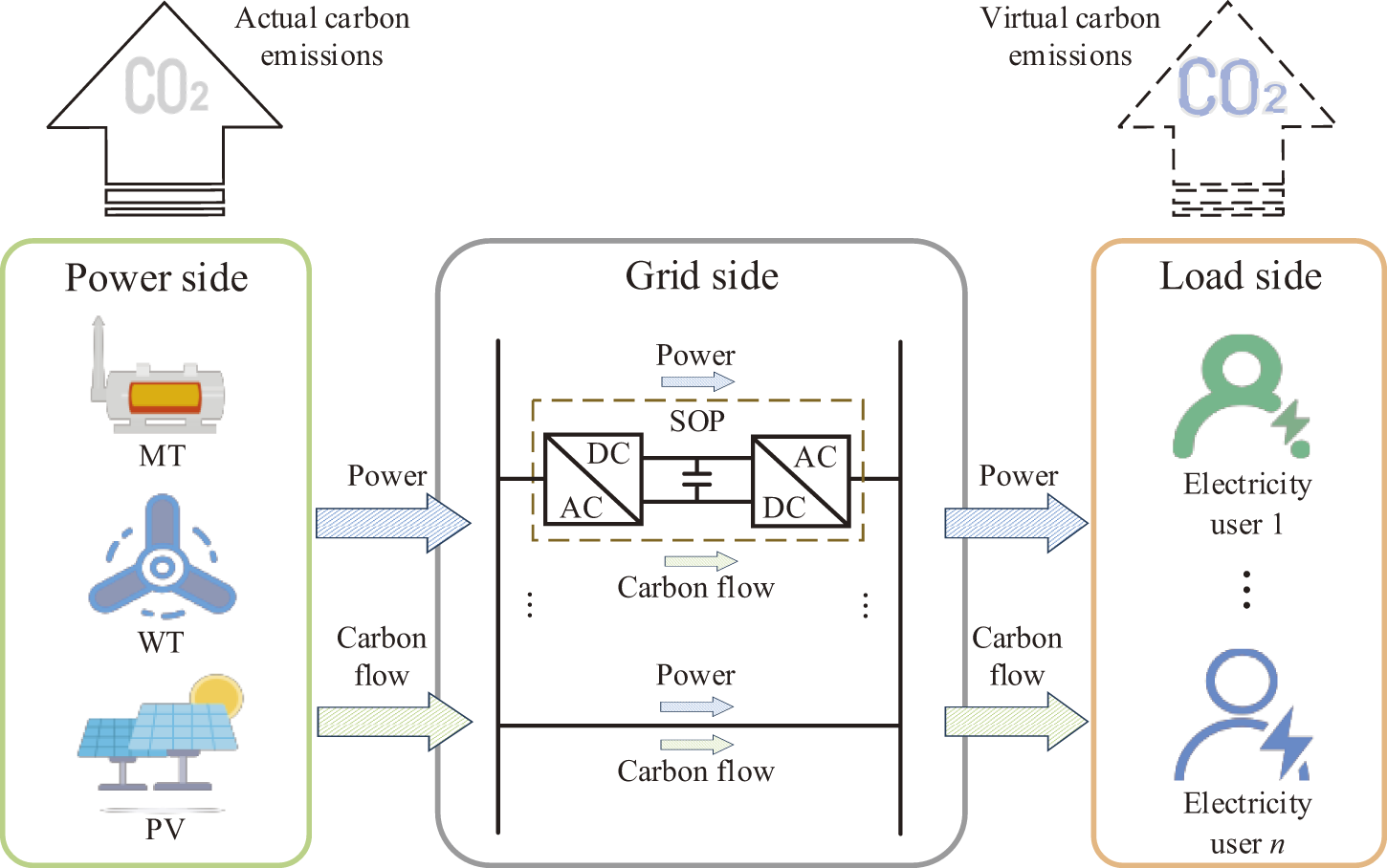
Figure 1: Schematic materialization of carbon emission flow in the power system
2.2 Theoretical Foundations of Power System Carbon Emission Flow: Definitions
CEF is a new concept and indicator, formed by adding carbon emission labels on the basis of grid active current data [22].
1) Branch Carbon Flow (BCF): It represents carbon emissions via branch l as active power flow passes through it, denoted as El, measured in gCO2.
2) Branch Carbon Flow Rate (BCFR): It is the carbon flow rate via branch l per unit time under active current, expressed as Rl in gCO2/h, as shown in Eq. (1).
3) Branch Carbon Flow Density (BCFD): It refers to the ratio of carbon flow rate via a branch to the active tidal current of that branch, expressed as IL,l and measured in gCO2/(kW·h), as shown in Eq. (2).
4) Node Carbon Emission Intensity (NCEI): It is used to describe the magnitude of the node’s carbon emission intensity, denoted by IN,i and measured in gCO2/(kW·h), as shown in Eq. (3).
The carbon flow density of tributary currents emanating from a node equals the node’s carbon emission intensity, as shown in Eq. (4).
2.3 The Ideas and Steps for Calculating Carbon Emission Flows from Power Systems
After the basic current calculation for the whole system, the data of nodes and branches of the whole network can be derived. The fundamental steps for calculating the carbon emission flow within a power system are as follows:
1) Determine the system tidal current distribution by basic tidal current calculation.
2) Determine the type of unit, and also determine the carbon emission factor data of each unit.
3) Based on the unit’s power generation, the carbon flow rate of the connected branches and the nodal carbon potential are extrapolated.
4) Derive the system carbon flow distribution after projecting to the load side.
3 Improved Carbon Flow Calculation Method for Flexible Distribution Networks
3.1 Characterisation of Carbon Flows in Flexible Distribution Networks
The DN has obvious radial characteristics. When DGs and the SOP are not connected and network loss is ignored, the inflow current of each node in the DN is only provided by its upstream node and the carbon emission intensity of all nodes is equal to that of the nodes of the transmission network (TN) connected to the DN. After the DGs and the SOP are connected to the DN, both of them change the distribution of currents in the FDN, which influences the carbon emission intensity of the nodes involved, ultimately impacting the CEF distribution across the entire FDN.
3.2 CEF Models Considering Intelligent Soft Open Point
Taking fully controllable power electronic devices as a basis, the SOP can replace the contact switch in DNs, enabling the regulation of active power and the compensation of reactive power across feeders, so as to regulate the current distribution of the whole DN. The location of the SOP access is shown in Fig. 2.
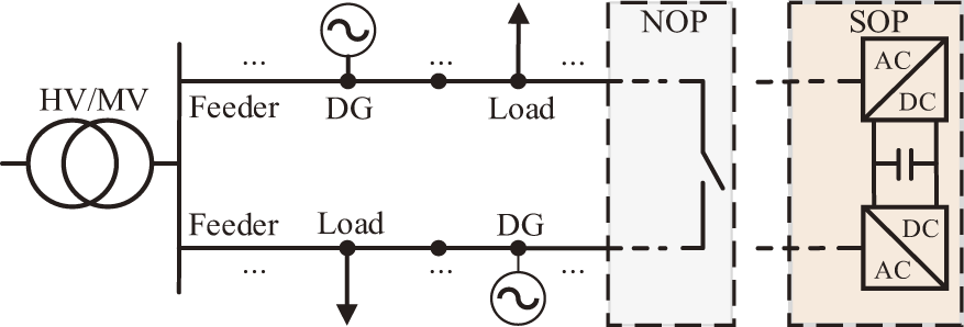
Figure 2: SOP access location map
The two ends of the SOP are respectively connected to nodes i and j of the DN, and the related operational constraints are presented as Eqs. (5)–(7) [23].
The power flows from one node of the SOP to the other and the CEF is dependent on the power flow in the DN. Therefore, the SOP can be regarded as a “branch circuit” that allows active power to pass through and can emit reactive power. When the SOP regulates active power in the DN, it can also regulate the distribution of carbon emissions within the DN. The CEF model considering a SOP is shown in Fig. 3.
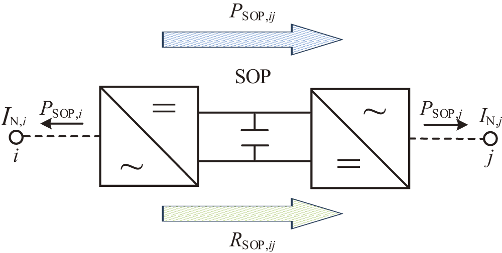
Figure 3: Schematic diagram of the carbon emission flow model considering a SOP
Based on the relevant characteristics of the SOP and the relationship between NCEI and BCFD, the formula for calculating the rate of carbon flow through the SOP is obtained as shown in Eqs. (8)–(11).
In the carbon flow model considering the SOP, the power loss of the converter at nodes i and j is ignored, as well as the loss of carbon emission. Eq. (8) is the active power balance equation of the SOP when converter losses are neglected, Eq. (9) represents the power magnitude relationship between nodes i and j of the SOP injection, Eq. (10) is the formula for the carbon flow density of the SOP, and Eq. (11) is the formula for the magnitude of the rate of carbon flow through the SOP.
where PSOP,ij represents the actual active power flowing from node i to node j in the SOP; ISOP,ij represents the carbon flow density in the SOP; RSOP,ij represents the carbon flow rate flowing through the SOP.
3.3 Carbon Flow Calculations for Flexible Distribution Networks
The calculation of CEFs is based on the key matrices and vectors defined in Table 1 [18].

The carbon intensity vector EG of the statistical power generation unit is used to calculate the carbon intensity vector EN of each node in the FDN, as shown in Eq. (12).
1) Power-side CEF calculations
To determine the amount of carbon emissions from power generation, the carbon intensity of the DG is multiplied by the active power injected by the DG into the FDN.
2) Network-side CEF calculations
The BCFR distribution matrix RB is obtained from the branch current distribution matrix PB, as shown in Eq. (13).
3) Load-side CEF calculations
The vector RL representing the carbon flow rates of the load is derived from the load distribution matrix PL, as indicated in Eq. (14).
4 Low-Carbon Optimal Operation Model for Flexible Distribution Networks
This section constructs an optimal operational model for the FDN that focuses on low-carbon emissions on the basis of carbon flow.
The objective functions include minimizing the generation cost, TN power purchase cost, network loss cost, and carbon emission cost, as shown in Eqs. (15)–(18).
1) The generation cost f1 is minimized as:
where cMT, cWT and cPV represent the cost of electricity generation per unit issued by the respective DGs, which includes micro-turbine (MT), wind turbine (WT), and photovoltaic (PV).
2) The TN power purchase cost f2 is minimized as:
where λi,t represents the unit cost of power purchased from the TN by FDN
3) The network loss cost f3 is minimized as:
where cLoss represents the unit cost of FDN network losses.
4) The carbon emission cost f4 is minimized as:
where πc represents the price of carbon emissions per unit.
The total cost f is shown in Eq. (19).
Constraints encompass AC distribution power flow limitations derived from the DistFlow model [24], constraints related to SOPs, and constraints in the carbon flow model.
1) Constraints on nodal power balance:
Constraint (20) denotes the AC power balance of node i.
where rki represents the resistance of branch ki, and xki represents the reactance of branch ki.
2) Voltage balance constraints:
3) Branch circuit current constraints:
To streamline the model, we apply second-order cone (SOC) relaxation [25,26] to the line power flow constraints, as shown in Eq. (23).
4) Branch circuit capacity constraints:
5) DG operational constraints:
6) SOP operational constraints:
Due to the nonconvexity and nonlinearity of Eqs. (6) and (7) in the original model, the optimization model constructed is non-convex. Thus, the above model is convexified in this subsection. Since Eqs. (6) and (7) are quadratic nonlinear constraints, Eqs. (6) and (7) are reformulated as SOC constraints, as shown in constraints (26) and (27).
7) Load node carbon emission equation constraints:
Constraint (28) formulates the real-time calculation of carbon emissions at the load node, which establishes a foundational basis for the subsequent analysis of carbon emission outcomes within the FDN.
8) Tributary carbon flow density constraints:
Constraint (29) describes the relationship between the density of tributary carbon flows out of a node and the intensity of carbon emissions at that node, which two are equal in magnitude.
9) Nodal carbon emission intensity equation constraints:
Constraint (30) represents the carbon emission intensity formula for node i in the FDN, where node i receives not only the power transmitted from the branch but also the power transmitted from the SOP.
The system has 33 nodes and 32 branch circuits, with a base voltage of 12.66 kV, and a maximum electrical load of 3715 kW. The model is solved using the GUROBI solver within the MATLAB software environment.
In this paper, the arithmetic example implements a modified IEEE 33-node DN and considers the installation of SOPs at the contact switches between feeders, as shown in Fig. 4.
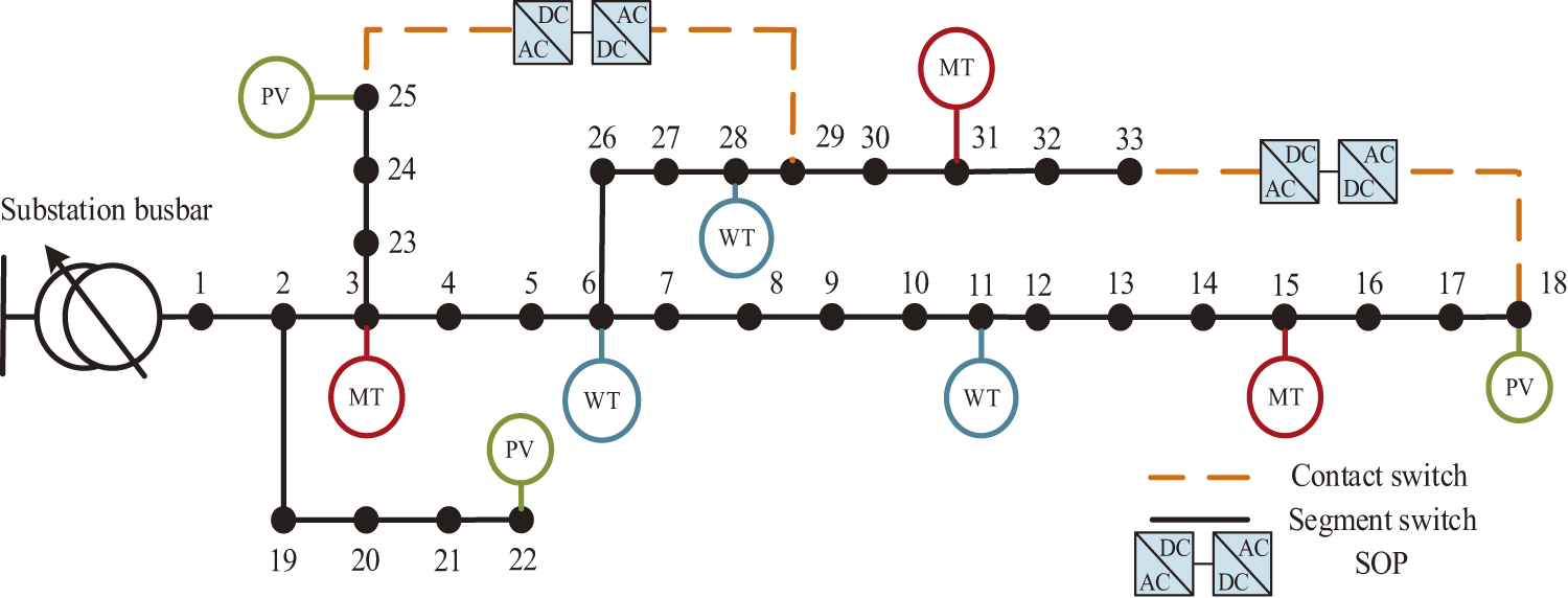
Figure 4: Improved IEEE 33-node distribution network
Table 2 displays the pertinent parameters of DG.

Fig. 5 illustrates the carbon emission intensity of the TN for each time period.
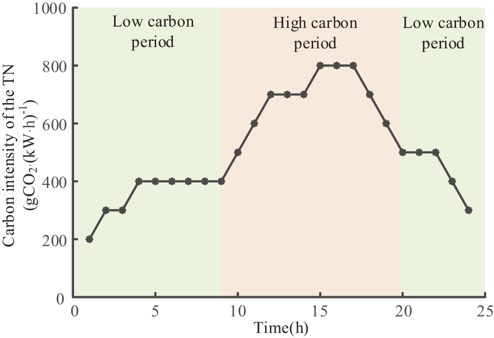
Figure 5: Carbon emission intensity of the transmission network by time period
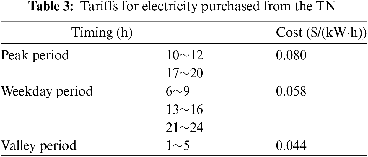
The unit cost of purchasing power from the TN by the DN for each time period is shown in Table 3.
Three cases are established for comparative analysis:
Case 1: failure to consider low-carbon elements in the operation of the DN.
Case 2: consider low-carbon elements in the DN operation process and optimize the carbon emission costs embedded in the objective function.
Case 3: based on Case 2, SOPs are installed at distribution branch circuits 18–33 and 25–29 to investigate the impact of the coordinated operation of DGs and SOPs on the low-carbon operation of FDNs.
1) Cost comparisons: The costs of the above cases were obtained as shown in Table 4.

DGs in the DN are distributed in a decentralised manner, and in Case 1 without considering the low-carbon element, the MT output is almost full in order to reduce the network loss of the DN, whereas after embedding the carbon cost in the objective function, the MT will adjust its own output during the day. The output of MT in each period under Case 2 is shown in Fig. 6. In the low-carbon period, the power transmitted from the TN to the DN contains more low-carbon power, MT does not generate power at this time. In the high-carbon period, the carbon emission intensity of the TN is always maintained at a high level, and to reduce the carbon emissions of the DN, MT will start to generate electricity and gradually increase its own output.
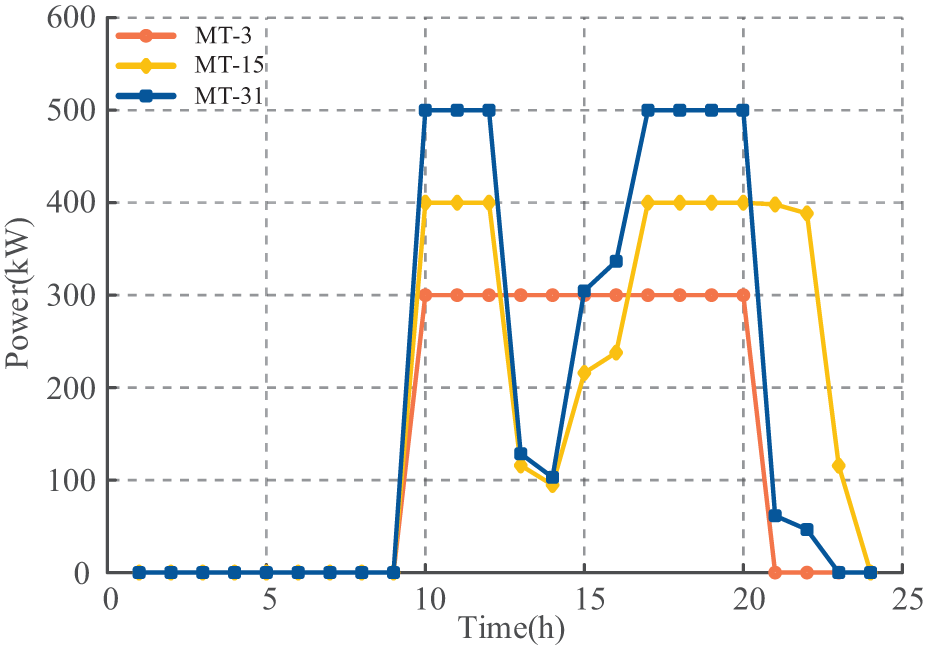
Figure 6: Real-time contribution of MT under Case 2
Combined with Table 4, Case 2 reduces the cost of electricity generation by 40.29 percent and the cost of carbon emissions by 10.02 percent compared to Case 1, demonstrating the need to consider low-carbon elements in the operation of the DN. Case 3 installs SOPs at DN branches 18–33 and 25–29 on the basis of Case 2. The generation cost, network loss cost and carbon emission cost are reduced under Case 3. This is due to the fact that the SOP can continuously control the power in the DN, which improves the ability of the DN to consume DG, especially the new energy units in close proximity to the network, and reduces carbon emissions while reducing network losses in the DN.
The active power transmitted on the SOPs under Case 3 is shown in Fig. 7. The TN is in a low carbon period in the early morning or evening moments, when the carbon potential of the TN is lower than that of the MT. The SOP close to the TN transmits low carbon power at that moment under the premise of ensuring reliable power supply. The low carbon power from the TN flows into the DN and transmits to node 25 and then transmits to node 29 through the SOP, which effectively balances the feeder loads and reduces the network losses while meeting the low-carbon demand of the DN loads. The SOPs installed at branches 18–33 are far away from the TN, so there is almost no active power transmission from these SOPs during the low carbon period of the TN. In addition, combined with the improved topology diagram of the IEEE 33-node distribution network, it can be seen that the SOPs installed at branches 18–33 and 25–29 are connected to a PV at one end. The PV is close to full generation when there is sufficient light, at which time the SOPs can transmit zero-carbon electricity in a timely manner.
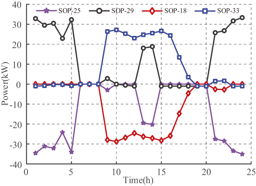
Figure 7: Active power transmitted on the SOP under Case 3
2) Analysis of carbon emission results: The individual cases were analyzed to obtain a one-day graph of variation in the NCEI, as shown in Fig. 8.
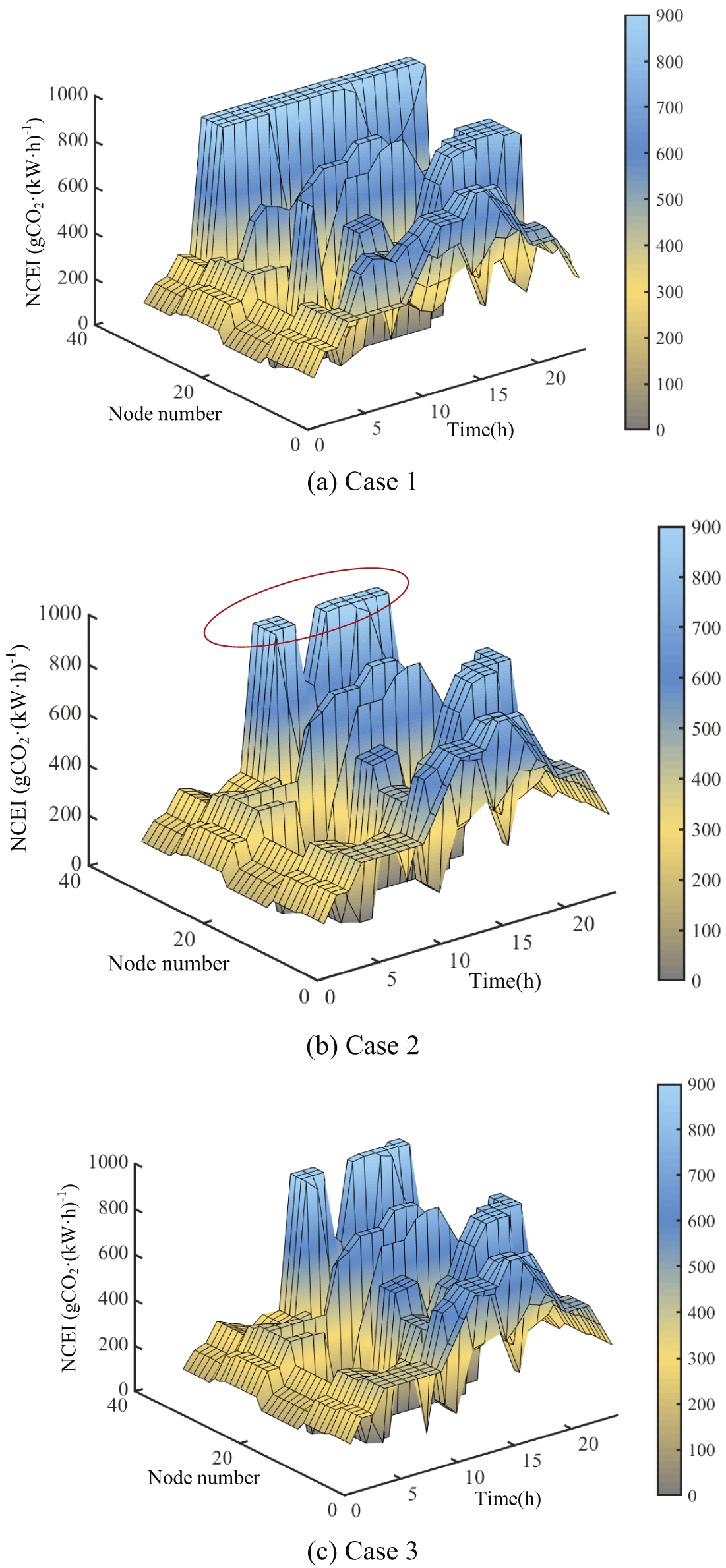
Figure 8: NCEI comparison chart
As shown in Fig. 8, different nodes in the DN exhibit large differences in nodal carbon emission intensity due to the different types of DG accessed and the influence of nearby nodes. There are more high coal-consuming units or those close to the TN installed near the high carbon emission intensity nodes in the DN, while more new energy units or those far away from the TN are installed near the low-carbon emission intensity nodes. When low-carbon elements are considered in Case 2, MTs do not input power into the DN during low-carbon periods, whereas during high-carbon periods, the MTs with low carbon intensity generate as much power as possible at full capacity, and the MTs with higher carbon intensity will regulate the level of output relative to their own carbon intensity and the carbon emission intensity of the TN, in order to minimize the use of high-carbon intensity thermal power from the TN.
Compared to Case 1, each node within the region of nodes 1–5 under Case 2 receives more low-carbon electricity from the TN during low-carbon periods, which results in a significant decrease in the carbon emission intensity of nodes within this region. In addition, nodes in the region of nodes 29–33 are connected to MT-31, and since MT-31 has a higher carbon intensity, it reduces its own output as much as possible during high-carbon periods, while the nodes in this region also receive low-carbon electricity from the TN. CEF is dependent on active power, and after the DN is configured with SOPs, nodes 29 and 33 and their neighbouring nodes receive zero-carbon electricity from PVs at the same time as when they receive active power transmitted by SOPs at the moment of sufficient light. Compared to Case 2, the carbon emission intensity of nodes in the region near the SOP under Case 3 is further reduced, and the number of nodes in the FDN with NCEI of 0 is further increased.
To analyze the contribution of the TN as well as the DG to the carbon flow rate at the load node, the moment t = 14 h is selected for different cases, as shown in Fig. 9.
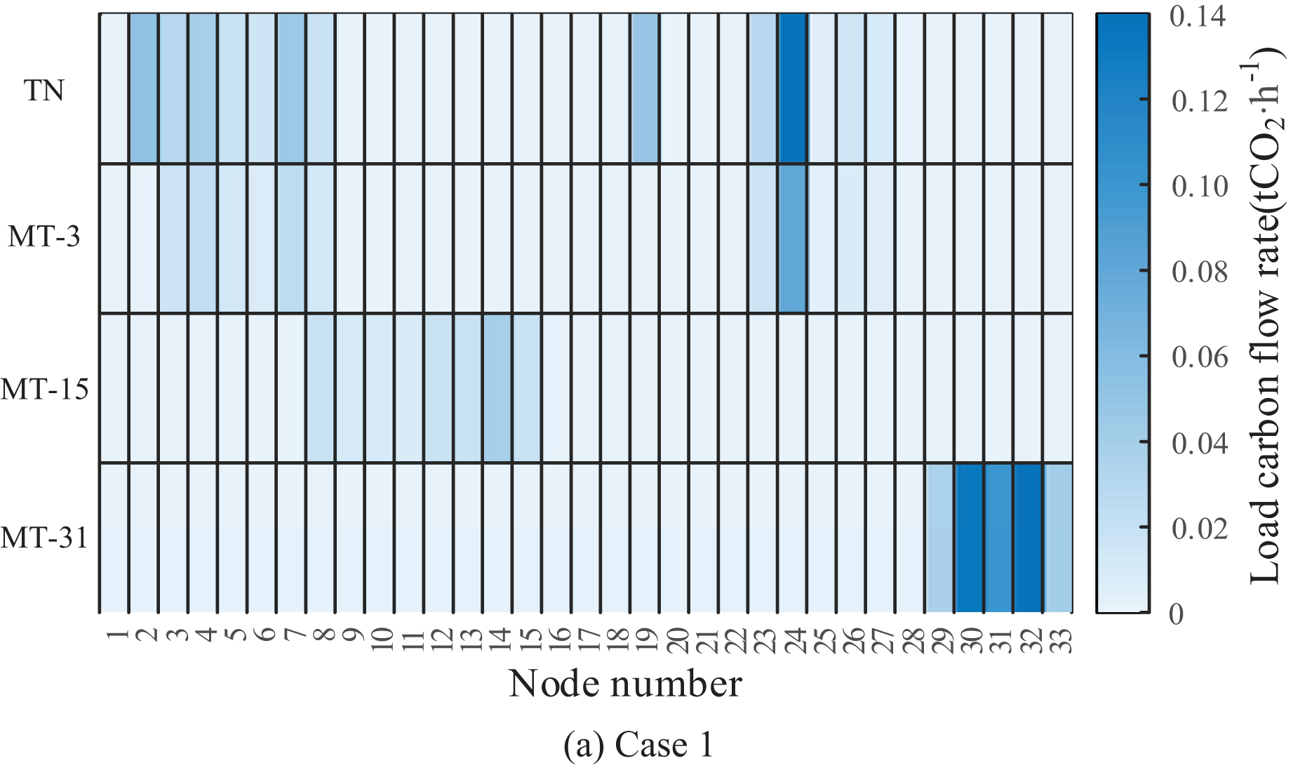
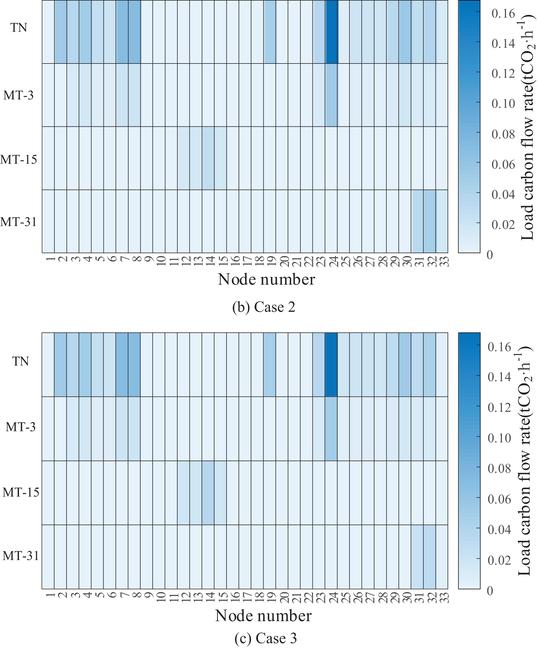
Figure 9: Load carbon flow rate distribution map
Node 1 in the DN is not connected to any load, thus it bears no carbon emission responsibility; the TN and MT do not contribute to the carbon flow of node 1. Furthermore, the load power of some nodes is supplied by renewable energy units, hence no carbon emissions are generated. Compared to Case 1, due to the reduced output of MT-31 in Case 2, there is a shift in the source of carbon flow rates for loads in the node 29–33 area. Thus, the carbon flow rate distribution in the DN becomes more balanced. With the addition of SOP, the traditional DN transitions from a “closed-loop design, open-loop operation” state to flexible closed-loop operation based on the SOP’s flexible interconnection technology, further enhancing the network’s decarbonization effectiveness.
This paper explores a low-carbon optimal operation approach for FDN on the basis of CEF. Taking into account the operational traits of SOP and DG, an improved model is constructed to optimize the FDN by strategically managing areas with significant carbon emissions. The key findings are as follows:
1) An improved low-carbon optimal operation method of FDN is proposed, which provides a reliable theoretical basis for the study of low-carbon optimal operation of FDN. When the SOP is connected to the DN, based on the traditional CEF model, it is regarded as a “branch circuit” that allows active power to pass through and can generate reactive power.
2) The low-carbon optimal operation model of FDN is established by the comprehensive consideration of the characteristics of DG and SOP. By analyzing the NCEI and load carbon flow rate distribution of the whole network, the areas with larger carbon flow rate in the DN are reasonably optimized, which effectively improves the economy of DN operation.
3) A comparative analysis of the cases reveals that when DG and SOP are operated in a coordinated manner in the FDN, the costs of power generation, network losses and carbon emissions are reduced, with the cost of carbon emissions being reduced by 10.18 percent. The results show that the coordinated operation of DG and SOP can achieve economic and low-carbon operation of the FDN.
This paper subsequently considers the introduction of artificial intelligence technologies, such as machine learning and deep learning, to intelligently dispatch and optimize the power network to achieve efficient energy allocation and low carbon emissions. At the same time, the cooperative operation strategy of distributed energy and smart grid is studied to improve the utilization rate of renewable energy and the stability of the network.
Acknowledgement: I would like to thank my mentor and siblings, who were instrumental in the successful completion of this work, for their unwavering encouragement and understanding throughout this project.
Funding Statement: This work was supported in part by National Natural Science Foundation of China under Grant 52007026.
Author Contributions: The authors confirm contribution to the paper as follows: study conception and design: Chao Gao and Kai Niu; data collection: Kai Niu and Wenjing Chen; analysis and interpretation of results: Changwei Wang, Wenjing Chen, Yabin Chen and Kai Niu; draft manuscript preparation: Kai Niu and Rui Qu. All authors reviewed the results and approved the final version of the manuscript.
Availability of Data and Materials: The authors ensure the authenticity and validity of the materials and data in the article.
Ethics Approval: Not applicable.
Conflicts of Interest: The authors declare no conflicts of interest to report regarding the present study.
References
1. S. Yang, W. S. Wang, C. Liu, and Y. H. Huang, “Optimal reactive power dispatch of wind power plant cluster considering static voltage stability for low-carbon power system,” J. Modern Power Syst. Clean Energy, vol. 3, no. 1, pp. 114–122, Mar. 2015. doi: 10.1007/s40565-014-0091-x. [Google Scholar] [CrossRef]
2. Q. Chen, C. Kang, Q. Xia, and J. Zhong, “Power generation expansion planning model towards low-carbon economy and its application in China,” IEEE Trans. Power Syst., vol. 25, no. 2, pp. 1117–1125, May 2010. doi: 10.1109/TPWRS.2009.2036925. [Google Scholar] [CrossRef]
3. H. Wang, W. Wang, and W. Zhao, “Carbon abatement cost-sharing strategy for electric power sector based on incentive and subsidy mechanisms,” Energy Eng., vol. 121, no. 10, pp. 2907–2935, Sep. 2024. doi: 10.32604/ee.2024.052665. [Google Scholar] [CrossRef]
4. S. Conti, R. Nicolosi, S. A. Rizzo, and H. H. Zeineldin, “Optimal dispatching of distributed generators and storage systems for MV islanded microgrids,” IEEE Trans. Power Del., vol. 27, no. 3, pp. 1243–1251, Jul. 2012. doi: 10.1109/TPWRD.2012.2194514. [Google Scholar] [CrossRef]
5. Y. Huang et al., “Bi-level coordinated planning of active distribution network considering demand response resources and severely restricted scenarios,” J. Modern Power Syst. Clean Energy, vol. 9, no. 5, pp. 1088–1100, Sep. 2021. doi: 10.35833/MPCE.2020.000335. [Google Scholar] [CrossRef]
6. N. C. Koutsoukis, D. O. Siagkas, P. S. Georgilakis, and N. D. Hatziargyriou, “Online reconfiguration of active distribution networks for maximum integration of distributed generation,” IEEE Trans. Autom. Sci. Eng., vol. 14, no. 2, pp. 437–448, Apr. 2017. doi: 10.1109/TASE.2016.2628091. [Google Scholar] [CrossRef]
7. C. Wang, G. Song, P. Li, H. Ji, J. Zhao and J. Wu, “Optimal siting and sizing of soft open points in active electrical distribution networks,” Appl. Energy, vol. 189, no. 1, pp. 301–309, Mar. 2017. doi: 10.1016/j.apenergy.2016.12.075. [Google Scholar] [CrossRef]
8. H. Ji, C. Wang, P. Li, F. Ding, and J. Wu, “Robust operation of soft open points in active distribution networks with high penetration of photovoltaic integration,” IEEE Trans. Sustain. Energy., vol. 10, no. 1, pp. 280–289, Jan. 2019. doi: 10.1109/TSTE.2018.2833545. [Google Scholar] [CrossRef]
9. H. Zhao, W. Chen, G. He, and J. Wang, “A new shared module soft open point for power distribution network,” IEEE Trans. Power Electron., vol. 38, no. 3, pp. 3363–3374, Mar. 2023. doi: 10.1109/TPEL.2022.3224972. [Google Scholar] [CrossRef]
10. S. Hoseinzadeh, D. A. Garcia, and L. Huang, “Grid-connected renewable energy systems flexibility in Norway islands’ Decarbonization,” Renew. Sustain. Energ. Rev., vol. 185, no. 3, Dec. 2023, Art. no. 113658. doi: 10.1016/j.rser.2023.113658. [Google Scholar] [CrossRef]
11. Y. Wang, J. Qiu, and Y. Tao, “Optimal power scheduling using data-driven carbon emission flow modelling for carbon intensity control,” IEEE Trans. Power Syst., vol. 37, no. 4, pp. 2894–2905, Jul. 2022. doi: 10.1109/TPWRS.2021.3126701. [Google Scholar] [CrossRef]
12. J. Li, J. Wen, and X. Han, “Low-carbon unit commitment with intensive wind power generation and carbon capture power plant,” J. Mod. Power Syst. Clean Energy, vol. 3, no. 1, pp. 63–71, Mar. 2015. doi: 10.1007/s40565-014-0095-6. [Google Scholar] [CrossRef]
13. L. Sang, Y. Xu, and H. Sun, “Encoding carbon emission flow in energy management: A compact constraint learning approach,” IEEE Trans. Sustain. Energy, vol. 15, no. 1, pp. 123–135, May 2023. doi: 10.1109/TSTE.2023.3274735. [Google Scholar] [CrossRef]
14. X. Shen, J. Li, Y. Yin, J. Tang, W. Lin and M. Zhou, “Carbon emission factors prediction of power grid by using graph attention network,” Energy Eng., vol. 121, no. 7, pp. 1945–1961, Jun. 2024. doi: 10.32604/ee.2024.048388. [Google Scholar] [CrossRef]
15. H. A. Gil and G. Joos, “Generalized estimation of average displaced emissions by wind generation,” IEEE Trans. Power Syst., vol. 22, no. 3, pp. 1035–1043, Aug. 2007. doi: 10.1109/TPWRS.2007.901482. [Google Scholar] [CrossRef]
16. Y. Cheng, N. Zhang, Y. Wang, J. Yang, C. Kang and Q. Xia, “Modeling carbon emission flow in multiple energy systems,” IEEE Trans. Smart Grid., vol. 10, no. 4, pp. 3562–3574, Jul. 2019. doi: 10.1109/TSG.2018.2830775. [Google Scholar] [CrossRef]
17. C. Yang, J. Liu, H. Liao, G. Liang, and J. Zhao, “An improved carbon emission flow method for the power grid with prosumers,” Energy Rep., vol. 9, no. 1, pp. 114–121, Dec. 2023. doi: 10.1016/j.egyr.2022.11.165. [Google Scholar] [CrossRef]
18. C. Kang et al., “Carbon emission flow from generation to demand: A network-based model,” IEEE Trans. Smart Grid., vol. 6, no. 5, pp. 2386–2394, Sep. 2015. doi: 10.1109/TSG.2015.2388695. [Google Scholar] [CrossRef]
19. W. Wang, Q. Huo, H. Deng, J. Yin, and T. Wei, “Carbon responsibility allocation method based on complex structure carbon emission flow theory,” Sci. Rep., vol. 13, no. 1, 2023, Art. no. 1521. doi: 10.1038/s41598-023-28518-y. [Google Scholar] [PubMed] [CrossRef]
20. M. Rouholamini, C. J. Miller, and C. Wang, “Determining consumer’s carbon emission obligation through virtual emission tracing in power systems,” Environ. Progress Sustain. Energy, vol. 39, no. 1, 2020, Art. no. 13279. doi: 10.1002/ep.13279. [Google Scholar] [CrossRef]
21. J. Hong, L. Zhang, Z. Hu, W. Lin, and Y. Zou, “A robust system model for the photovoltaic in industrial parks considering photovoltaic uncertainties and low-carbon demand response,” Front. Energy Res., vol. 12, no. 1, 2024, Art. no. 1343309. doi: 10.3389/fenrg.2024.1343309. [Google Scholar] [CrossRef]
22. X. Wei, X. Zhang, Y. Sun, and J. Qiu, “Carbon emission flow oriented tri-level planning of integrated electricity-hydrogen–gas system with hydrogen vehicles,” IEEE Trans. Ind. Appl., vol. 58, no. 2, pp. 2607–2618, Mar./Apr. 2022. doi: 10.1109/TIA.2021.3095246. [Google Scholar] [CrossRef]
23. J. Wang, N. Zhou, C. Y. Chung, and Q. Wang, “Coordinated planning of converter-based DG units and soft open points incorporating active management in unbalanced distribution networks,” IEEE Trans. Sustain. Energy, vol. 11, no. 3, pp. 2015–2027, Jul. 2020. doi: 10.1109/TSTE.2019.2950168. [Google Scholar] [CrossRef]
24. M. E. Baran and F. F. Wu, “Optimal sizing of capacitors placed on a radial distribution system,” IEEE Trans. Power Del., vol. 4, no. 1, pp. 735–743, Jan. 1989. doi: 10.1109/61.19266. [Google Scholar] [CrossRef]
25. P. Li et al., “Coordinated control method of voltage and reactive power for active distribution networks based on soft open point,” IEEE Trans. Sustain. Energy, vol. 8, no. 4, pp. 1430–1442, Oct. 2017. doi: 10.1109/TSTE.2017.2686009. [Google Scholar] [CrossRef]
26. L. Bai, T. Jiang, F. Li, H. Chen, and X. Li, “Distributed energy storage planning in soft open point-based active distribution networks incorporating network reconfiguration and DG reactive power capability,” Appl. Energy, vol. 210, no. 2, pp. 1082–1091, Jan. 2018. doi: 10.1016/j.apenergy.2017.07.004. [Google Scholar] [CrossRef]
Cite This Article
 Copyright © 2025 The Author(s). Published by Tech Science Press.
This work is licensed under a Creative Commons Attribution 4.0 International License , which permits unrestricted use, distribution, and reproduction in any medium, provided the original work is properly cited.
 Downloads
 Citation Tools