Joint Estimation of SOH and RUL for Lithium-Ion Batteries Based on Improved Twin Support Vector Machineh

1  Introduction

Global climate change and growing energy demand are driving changes in the energy sector. The proliferation of lithium-ion battery (LIB) storage systems and their associated technologies has been pivotal, not only altering energy consumption patterns but also electrifying traditional energy sources [1]. However, safety hazards in energy storage systems have resulted in numerous incidents, such as the Samsung Note 7 battery explosion and the lithium battery mobile power supply fire on China Southern Airlines flight CZ3539. Aging and performance degradation of LIBs are the underlying causes of these safety issues [2]. Therefore, battery management systems (BMS) capable of comprehensively monitoring and protecting LIBs have become essential [3]. The State of Health (SOH) and Remaining Useful Life (RUL) serve as crucial indicators within BMS for assessing LIBs’ aging and performance degradation [4]. SOH reflects the gradual decrease in LIBs’ capacity, as shown in Eq. (1) [5].

SOH=QnQ0(1)

where Qn is the capacity of LIBs at that time; Q0 is the initial capacity of the LIBs.

Determining the SOH is a critical step in predicting the RUL of a LIB. RUL refers to the number of cycles a battery can perform under certain cycling conditions before its SOH decreases to the operational limit. A LIB is typically considered to be at the end of its useful life when its SOH first falls to 0.8. To accurately and reliably estimate the SOH and RUL of lithium batteries, researchers have proposed three main methods: experimental analysis, model-based approaches, and data-driven approaches. The experimental analysis method uses experimental setups to obtain parameters such as internal resistance, capacity, and electrochemical impedance spectroscopy (EIS) of lithium batteries for SOH and RUL measurement [6], as in the Coulomb counting method described in literature [7]. This method evaluates the SOH of lithium batteries by dynamically recalibrating the maximum releasable capacity. In literature [8], EIS is used to determine SOH by calculating the ratio of the zero-crossing real part of the Nyquist plot to the low-frequency inflection point real part. This method offers high prediction accuracy and simplicity in principle but shows relatively poor generalization performance. Model-based approaches estimate the SOH of lithium batteries by establishing electrochemical or equivalent circuit models and combining them with filtering algorithms. For example, the research described in [9] applies an improved Remora algorithm to fine-tune the parameters of a first-order RC equivalent circuit for lithium batteries. This is followed by employing a dual adaptive Kalman filtering algorithm to estimate the SOH. However, model-based techniques demand a thorough grasp of the basic physics and chemistry, which can be challenging when attempting to capture the complex dynamic and static properties of LIBs [10]. Data-driven methods do not require in-depth analysis of the internal aging mechanisms of lithium batteries but instead extract features from historical data to establish SOH prediction models [11,12]. Currently, widely used methods for SOH and RUL estimation include Support Vector Machines (SVM) [13], Long Short-Term Memory networks (LSTM) [14], Extreme Learning Machines (ELM) [15], and Gaussian Process Regression (GPR) [16]. In [17], the Variable Forgetting Factor Online Sequential Extreme Learning Machine (VFOS-ELM) was utilized to estimate the SOH of LIBs. Meanwhile, Reference [18] used incremental capacity curves as inputs for a neural network model, employing a Convolutional Neural Network (CNN) to extract features and proposing a CNN-LSTM model with skip connections to enhance prediction accuracy. Literature [19] proposed a hybrid model combining a Temporal Convolutional Network (TCN) and LSTM, demonstrating robustness and generalization capabilities.

With the widespread use of data-driven methods, an increasing number of studies have utilized SVM and modal decomposition to predict the SOH and RUL of LIBs. Literature [20] extracted Health Indicators (HIs) from time intervals of equal charging voltage differences and equal discharging voltage differences, employing SVM for SOH and RUL prediction. Literature [21] proposed a method for optimal selection of SVM parameters based on particle swarm optimization (PSO), effectively capturing the degradation trend of LIBs. Nevertheless, SVM necessitates the resolution of a pair of quadratic programming problems, which introduces additional variables and constraints, expands the scope of the problem, and increases the computational complexity. This poses significant challenges, especially when dealing with high-dimensional complex datasets. In contrast, literature [22] decomposed the discharge capacity of LIBs into two components: global degradation trends and capacity regeneration, using empirical mode decomposition (EMD). Although EMD and its variants are used to predict the degradation trend of LIBs, they struggle with insufficient decomposition and modal overlap when targeting highly complex sequences [23]. Literature [24] utilized Variational Mode Decomposition (VMD) to separate the capacity of LIBs into overall deterioration tendencies and local stochastic contributions, modeling them via an Echo State Network (ESN) and Bayesian Optimized LSTM, respectively. The RUL predictions are derived by integrating these models. However, it is important to note that VMD is not a specialized noise reduction tool. Consequently, noise may persist in certain modal components, potentially affecting the accuracy of predictions.

When applying the prediction model, the setting of relevant parameters plays a crucial role in the prediction results. Traditional deterministic optimization algorithms often face slow convergence speeds and other issues when dealing with discontinuous and non-differentiable functions. Literature [25] proposed the convolution optimization algorithm (COA), a new intelligent optimization algorithm that incorporated a two-dimensional convolution operation into the population position updating process of intelligent optimization algorithms. This algorithm includes two mechanisms: convolution search and de-quality enhancement. This approach has demonstrated good convergence speed, stability, and optimization ability. However, COA may encounter issues with uneven initial population and susceptibility to local optimization.

To address the above shortcomings, this paper improves the COA algorithm and proposes a joint SOH and RUL prediction method based on VMD-RF-ICOA-TWSVM. The main contributions are summarized as follows:

a) Extract the constant-current charging time of LIBs as health indicator (HI), decompose the extracted HI into modal components with different frequency-domain features by using VMD, and adopt Random Forest (RF) importance ranking for noise reduction and model complexity reduction.

b) Introduce the good point set method to optimize the initial population and the differential evolution method in the solution enhancement stage to strengthen the global optimality searching ability, solving the problem of the inhomogeneous initial population of COA and its tendency to fall into local optima.

c) To address the issue of SVM computation complexity, the improved COA algorithm is utilized to optimize the twin support vector machine model for joint prediction of SOH and RUL.

The paper is structured as follows: Section 2 focuses on related techniques and theories, Section 3 describes the data processing process, Section 4 discusses the simulation of the prediction model, and Section 5 provides a summary of the paper.

2  Methodology

2.1 Variational Modal Decomposition (VMD)

VMD is an efficient signal processing method for nonsmooth signals [26]. The signal decomposition is transformed into the solution of unbounded discretization problems by the adaptive identification of the corresponding frequencies and the evaluation of the respective modes to compensate for the error.

The charging time of LIBs is influenced by stochastic effects such as the capacity degradation trend and the relaxation effect. To better understand the changes in battery performance, it is helpful to use VMD decomposition to extract modal components and obtain multi-scale degradation features. The charging time data is decomposed into intrinsic modal functions (IMFs) and Residual (R) at different frequencies using VMD [27]. The IMFs represent factors such as stochastic fluctuations and capacity regeneration, while R presents the overall trend of the capacity change. VMD constructs and solves the variational problem that determines the eigenmode functions at each iteration by minimizing a regularized constraint function. Each function corresponds to an eigenfrequency in the signal. The constrained variational model expression for the signal f(t) is shown in Eq. (2):

f(t)=min{un},{ωn}{∑n=1N‖∂n[un(t)∗(δ(t)πt+jπt)]e−jωnt‖22}s.t.∑n=1Nun(2)

where ∂n is the signal gradient; {un} is the modal component; {ωn} is the center frequency; * denotes the convolution; δ(t) is the unit pulse signal; N is decompositions number.

To cope with the constraints in the computational process, Lagrange multiply factor α and the penalty factor λ are introduced to change the constraint variational solution problem into the unbounded form as shown in Eq. (3):

L({un},{ωn},λ)=α{∑n=1N‖∂t[un(t)∗(δ(t)πt+jπt)]e−jωt‖22}+‖f(t)−∑n=1Nu(t)‖22+⟨λ(t),f(t)−∑n=1Nun(t)⟩(3)

The multiplicative alternating algorithm is adopted to continuously update each modal component and center frequency until the iteration is made to satisfy the convergence condition, as shown in Eqs. (4) and (5):

u^nk+1(ω)=f^(ω)−∑i≠nu^(ω)+λ^(ω)21+2α(ω−ωn)2(4)

ω^nk+1=∫0∞ω|u^n(ω)|2dω∫0∞|u^n(ω)|2dω(5)

u^nk+1 is the n-th mode with center frequency ω at iteration k + 1; ω^nk+1 is the average center freq of the k-th mode at iteration k + 1.

2.2 Importance of Random Forest Features (RF)

Although VMD is effective in handling nonlinear and nonsmooth signals, it is sensitive to noise and lacks noise reduction. Therefore, this paper proposes the use of RF to rank the importance of IMFs and R, remove modal components that contain noise or have less influence, and retain key modal components as final inputs. This method reduces the feature dimension, simplifies the model, and reduces the risk of overfitting [28]. Random Forest is a classifier that integrates Bagging and consists of multiple fully grown decision trees. The training set for each decision tree is randomly sampled from the original data, and some of the samples constitute out-of-bag (OOB) data, which is used to calculate feature importance. This strategy improves the model’s conciseness and generality.

In RF, the importance of feature x can be derived by the following steps: first, generate the training set and dataset OOB using self-service resampling, and construct the decision tree Tk on the training set; second, use Tk to predict the classification of the OOB data and count the number of correctly classified samples, which is noted as Rk; next, perturb the value of feature x in the OOB noisily to obtain a new OOB sample set, and then use Tk to classify the new OOB sample set for prediction and count the number of correctly classified samples, denoted as Rk′; finally, the process is repeated (k = 2,3, ..., K), and the importance of feature a is shown in Eq. (6):

IM(x)=1K∑k=1K(Rk−Rk′)(6)

A significant decrease in the accuracy of the out-of-bag data (i.e., a decrease in Rk′) caused by noise perturbation indicates that the feature has a substantial impact on the sample prediction results, signifying its high importance. Conversely, if the decrease is minimal, it indicates that the feature’s impact is limited.

2.3 Improved Convolution Optimization Algorithm ( ICOA)

2.3.1 Population Initialization

To enhance the global search capabilities of the COA, this paper employs the benefits of good point set theory to uniformly distribute points. This method ensures a more uniform initial population, thereby improving the COA’s global optimization search performance. The theory of good point sets is proposed by the Chinese mathematician Hua Luogeng and others. Its principle assumes that Gs is a unit cube in an s-dimensional Euclidean space, within which there exists a point set as described in Eq. (7):

Pn(k)={({r1(n)⋅k},{r2(n)⋅k},⋯,{rs(n)⋅k}),1≤k≤n}(7)

Its deviation φ(n) satisfies φ(n)=C(r,ε)n−1+ε, where C(r,ε) is a constant related only to r and ε (ε is an arbitrary positive number), then Pn(k) is said to be the good point set and r is the good point. Fig. 1 shows the comparison between the original populated using the good point set and the random generation, the original populated using the good point set is more homogeneous compared to the random generation for the same population size.

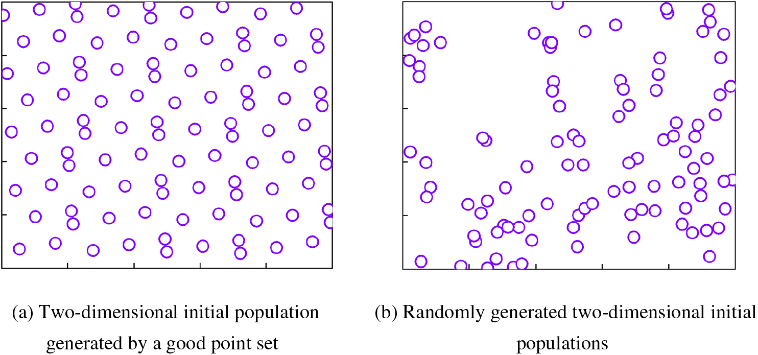
Figure 1: Population distribution map

The position of an individual Xp(p=1,2,…,n) is a candidate for solving the fitness solution, and the position vector X of the population consists of n individuals of dimension d. Then the position vector X of the population consists of an n×d-order matrix as shown in Eq. (8):

X=[X1⋮Xn]=[x11⋯x1d⋮⋱⋮xn1⋯xnd](8)

The fitness value of the position vector X of the population is shown in Eq. (9):

Fx=[f(X1)⋮f(Xn)]=[f([x11x12⋯x1d])⋮f([xn1xn2⋯xnd])](9)

2.3.2 Convolutional Search Process

The vertical, horizontal, and regional convolution kernels are defined during convolutional positioning as shown in Eq. (10):

{KL=2×rand(k,1)−ILKT=2×rand(1,k)−ITKR=2×rand(k,k)−IR(10)

where KL, KT, and KR represent the vertical, horizontal, and regional convolution kernels, respectively, each as a k×1, 1×k and k×k matrix. rand(1×k), rand(k×1), and rand(k,k) are matrices of the same dimensions, with each element being a random number between 0 and 1. IL, IT, and IR are k×1, 1×k, and k×k matrices with all elements equal to 1.

The vertical, horizontal, and regional convolutions are defined as shown in Eq. (11):

{XLt=Xt∗KLXTt=Xt∗KTXRt=Xt∗KR(11)

where t is the current iteration; Xt is an n×d matrix representing the population position vector at generation t. XLt, XTt, and XRt are n×d matrices representing the updated population position vectors after convolution at generation t. The best positions replace the individuals in EEE, as shown in Eqs. (12)–(14):

Xpt={XLpt,f(XLpt)<f(Xpt)Xpt, else (12)

Xpt={XTpt,f(XTpt)<f(Xpt)Xpt, else (13)

Xpt={XRpt,f(XRpt)<f(Xpt)Xpt, else (14)

where Xpt is the position of the pth individual in the population at generation t. XLpt, XTpt, and XRpt represent the pth individual’s position after convolutional updates at generation t.

In the integrated position update stage, the position vector XLt of the population after the longitudinal convolution update of generation t, the position vector XTt of the population after the transverse convolution update of generation t, and the position vector Xrt of the population after the regional convolution update of generation t, are merged into XSt by summing them using either random weights or equal proportional weights as shown in Eq. (15):

XSt=r1×XLt+r2×XTt+r3×XRtr1+r2+r3(15)

where r1, r2, and r3 are random numbers between [0, 1], and in particular, r1=r2=r3 can be made so that equal proportional weights are summed. The individual positions in Xt are replaced optimally as shown in Eq. (16):

Xpt={XSpt,f(XSpt)<f(Xpt)Xpt, else (16)

where XSpt is the p-th individual position of the population after the integrated position update in the t-th generation. Finally, the fitness values of all individual positions in Xt are calculated and ranked according to the size of the fitness values to select the optimal solution Xbst.

2.3.3 Solving Mass Enhancement Processes

In COA, the solution quality enhancement process is to perturb the d-dimensional search space of the optimal solution Xbst with Gaussian variation with non-inertial weights dimension by dimension, and perturb the optimal solution Xbst. However, the Gaussian variation with non-inertial weights can easily fall into the local optimal solution, and there is not enough diversity in the search of the solution space, so the authors switched to perturbation optimization searching for the optimal solution Xbst by using the differential evolution method, which is much more powerful for global searching, as shown in Eq. (17):

Xnbs(q)t=ω⋅Xqt+F⋅(Xbs(r1)t−Xbs(r2)t)(17)

where ω is the weight coefficient, F is the scaling factor, Xbs(r1)t and Xbs(r2)t are two n×1 order matrices, which are the randomly selected r1 and r2 (r1,r2∈(1,d))-dimensional locations in the d-dimensional search space of the optimal solution Xbst; ω=1−(t/itermax)2, where itermax represents the maximum number of iterations, and Xnbs(q)t is an n×1 matrix that represents the q-th dimension of the optimal solution Xbst after performing differential evolution on the q-th dimension. Let the individual position after differential evolution on the qth dimension be X(q)nbst, compare the magnitude of the fitness values of X(q)nbst and Xbst, and optimally replace the individual position of Xbst as shown in Eq. (18):

Xbst={X(q)nbst,f(X(q)nbst)<f(Xbst)Xbst, else (18)

2.4 Twin Support Vector Machine (TWSVM)

TWSVM improves performance significantly compared to traditional SVM by converting a large-scale quadratic programming problem into two smaller problems. This algorithm generates two non-parallel hyperplanes, f1(x)=ω1Tx+b1 and f2(x)=ω2Tx+b2, which respectively determine the upper and lower bounds of the insensitive function for the unknown regression variables. The final regression result is the average of the regression results of the two hyperplanes. For nonlinear problems, TWSVM uses a kernel function K to map samples into a high-dimensional space for linear regression. The two quadratic QP problem constructions of TWSVM are shown in Eqs. (19) and (20):

{min12‖Y−eε1−(K(A,AT)ω1+eb1)‖2+c1eTξS.T.Y−(K(A,AT)ω1+eb1)≥eε1−ξ,ξ≥0(19)

{min12‖Y+eε2−(K(A,AT)ω2+eb2)‖2+c2eTηS.T.(K(A,AT)ω2+eb2)−Y≥eε2−η,η≥0(20)

where A is the input of the training samples, Y is the output, c1 and c2 are the penalty coefficients, both of which are greater than 0, ε1 and ε2 are the optimization parameters, ξ and η are the slack variables, and e is the unit column vector of the corresponding dimension. Subsequently, Lagrange multipliers α,β are introduced to transform the original problem into the corresponding dual problem, and the quadratic QP problem represented by Eq. (19) is derived from Eq. (21) by the Karush-Kuhn-Tucker condition:

{∂L∂ω1=−K(A,AT)[Y−eε1−(K(A,AT)ω1+eb1)]+K(A,AT)Tα=0∂L∂b1=−eT[Y−eε1−(K(A,AT)ω1+eb1)]+eTα=0∂L∂ξ=c1e−α−β=0∂L∂α=Y−[K(A,AT)ω1+eb1]>eε1+ξ∂L∂β=αT[Y−(K(A,AT)ω1+eb1)−eε1+ξ]=0ξ≥0,α≥0,β≥0,βTξ=0(21)

The other quadratic QP problem is the same. The dyadic problems of the above equation can be changed as shown in Eqs. (22) and (23), respectively:

{max−12αTG(GTG)−1GTα+FTG(GTG)−1GTα−FTαS.T.0≤α≤c1e(22)

{max−12βTG(GTG)−1GTβ−HTG(GTG)−1GTβ+HTβS.T.0≤β≤c2e(23)

where F=Y−eε1, H=Y+eε2, G=[K(A,AT)e] and the parameters of the two hyperplanes of the TWSVM are shown in Eq. (24):

{u1=[ω1Tb1]=(GTG)−1GT(F−α)u2=[ω2Tb2]=(GTG)−1GT(H+β)(24)

In this paper, the polynomial kernel function K(xi,xj)=(xi⋅xj+u)d is chosen to map the data from the original feature space to the higher dimensional feature space, where xi⋅xj is the inner product of the feature vectors, u is the bias parameter, and d is the polynomial number. The final objective function is shown in Eq. (25):

f(x)=12[(ω1+ω2)TK(xi,xj)+(b1+b2)](25)

2.5 VMD-RF-ICOA-TWSVM Modeling

The choice of parameters is crucial in TWSVM predictive modeling. The penalty coefficient c balances the weight of the loss. A larger bias parameter u may cause the hyperplane to deviate from the origin in the feature space, and the polynomial degree d determines the complexity of the data mapping. To obtain optimal prediction results, ICOA is introduced for parameter optimization. The improved TWSVM flowchart is shown in Fig. 2 and the main steps are as follows:

a)   Acquire the data and extract the HI of the LIBs’ constant current charging time.

b)   Perform VMD modal decomposition of the HI to obtain the degradation characteristics of the LIBs at different scales. Subsequently, rank the importance of each modal component and trend term using random forest, and remove the modal components and trend terms containing noise and having little effect.

c)   The optimization process involves using ICOA to calculate the fitness value of each individual population in order to determine the location of the optimal individual population. Then, the differential evolution method is used to perturb the optimal individual position for further optimization and to determine the optimal individual position, resulting in the optimal parameters.

d)   The optimal parameters are input into TWSVM for model training to obtain the VMD-RF-ICOA-TWSVM prediction model.

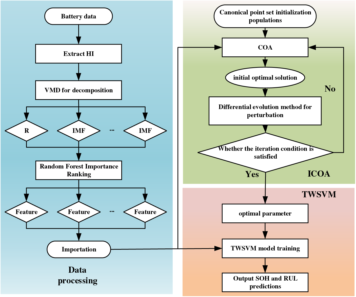
Figure 2: Flowchart of the improved support vector machine prediction model

3  Data Processing

3.1 Dataset and Health Feature Extraction

This study utilizes lithium battery data B0005, B0006, and B0007 provided by NASA PCoE, with initial capacities of 1.8565, 2.0353, and 1.8911 Ah, respectively. A total of 168 charge-discharge cycles were conducted at room temperature (24°C). During the charging phase, a constant current (CC) of 1.5 A was applied until the voltage reached 4.2 V, followed by a constant voltage (CV) phase. The discharging phase used a constant current of 2 A, stopping when the battery voltage dropped to 2.7, 2.5, and 2.2 V, respectively. Due to differences in battery types and experimental conditions affecting prediction accuracy, CS2-33, CS2-34, and CS2-36 lithium batteries from the CALCE dataset were used to validate generalization performance. These batteries underwent over 700 charge-discharge cycles, far exceeding the NASA dataset, representing short-life and long-life batteries. Fig. 3 shows the capacity degradation curves of the six lithium batteries, and Fig. 4 displays the constant current charging time curves. As the number of cycles increases, the constant current charging time gradually decreases. The battery capacity degradation and constant current charging time trends in the NASA and CALCE datasets are similar, making constant current charging time a viable HI.

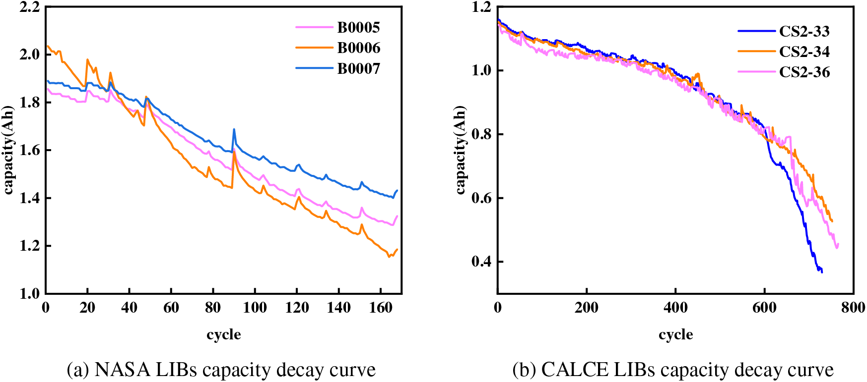
Figure 3: LIBs capacity decay curve

Figure 4: LIBs constant current charging time

3.2 Health Indicator Analysis

To capture the global degradation trend and local stochastic fluctuation components of the signal, VMD is employed for multi-scale decomposition of the HI. In the signal decomposition process of VMD, the parameter K denotes the number of modes selected for decomposing the signal. Choosing an appropriate K value is crucial for achieving high-quality decomposition results and effectively reducing computation time. Typically, the selection range for K values is between 2 and 10. In this study, K is set to 10 to maintain ample flexibility during the decomposition process, thereby comprehensively capturing the signal characteristics. By opting for a larger K value, more informative inputs are provided for the subsequent noise reduction step using random forests. Using NASA data from the B0005 lithium-ion battery as an example, Fig. 5 illustrates the decomposition results of the constant current charging time.

Figure 5: B0005 constant current charging time decomposition curve

As depicted in Fig. 5, R represents the global degradation trend, whereas IMF1 to IMF9 depict local capacity regeneration and random fluctuation characteristics. Therefore, the RF importance ranking is utilized to discard modal components that are insignificant and noisy for predictions, thereby emphasizing key signal components and enhancing the accuracy of SOH and RUL predictions.

The decision tree number is set to 50, the first 100 data are used as the training set, and the remaining 68 data are used as the test set, and the importance of the random forest features of the modal components of the three LIBs is shown in Fig. 6.

Figure 6: Random forest feature importance ranking

When calculating feature importance, positive values indicate that the feature has a significant positive impact on the model’s prediction target; increasing such features can enhance prediction performance. Negative values indicate that the feature has a substantial negative impact on the target; reducing such features can also improve prediction performance. Trends R and IMF9 show higher importance, whereas IMF3 and IMF4 for B0005, IMF2 and IMF6 for B0006, and IMF1 for B0007 exhibit minor influence on predictions and may include noise. Therefore, this study excludes modal components with absolute values less than 0.1, retaining the remaining modal components as feature inputs.

4  Analysis of Cases

4.1 Model Parameters and Evaluation Indicators

(1) Model parameters

The optimization parameters are the penalty coefficient c1, the bias parameter u1, and the polynomial number of times d1 for the first hyperplane, and the penalty coefficient c2, the bias parameter u2, and the polynomial number of times d2 for the second hyperplane. After repeated experiments, the optimization ranges were set to be c1∈[2−15,210], u1∈[2−15,210], d1∈[0,10], c2∈[2−15,210], u2∈[2−15,210], d2∈[0,10], the number of populations is set to 20, and the number of iterations is set to 10. In order to validate that the proposed method is applicable to the LIBs SOH and RUL prediction, respectively, the top 30% and top 50% of the LIBs data as the training set (the proportion of the training set is defined as T), and the other data as the test set for testing. After simulation, the parameters of TWSVM are shown in Table 1.

(2) Evaluation indicators

To assess the predictive effectiveness model, this study uses Root Mean Square Error (RMSE), Mean Absolute Percentage Error (MAPE) and Relative Error (RE) of RUL.

RMSE=1n∑i=1n(xi−xi^)2(26)

MAPE=1n∑i=1n|xi−xi^xi|×100%(27)

RE=PRUL−RULRUL×100%(28)

where xi is the real value, x^ is the predicted value, and n is data number. RUL indicates the remaining battery life; PRUL refers to the prediction of the remaining service life, and RE is greater than 0, which indicates that the predicted number of remaining cycles is higher than the actual one, which may lead to overuse of LIBs and threaten the system safety; and RE is less than 0, which indicates that the predicted number of remaining cycles is lower than the actual one, which may lead to under-utilization of LIBs and increase the unnecessary cost of replacing the batteries. If RE is less than 0, it means that the predicted number of remaining cycles is lower than the actual number. This may result in underutilization of the LIBs and unnecessary costs for battery replacement.

4.2 Results and Discussion

To verify the prediction accuracy of the proposed model, the VMD-COA-TWSVM and VMD-TWSVM models were selected for comparative illustration. Fig. 7 presents the SOH prediction curve and absolute error at T = 30%. It is observed that compared to other models, the predictions of VMD-RF-ICOA-TWSVM are closest to the real values, demonstrating a strong convergence effect and tracking ability. The maximum absolute errors for both VMD-TWSVM and VMD-COA-TWSVM are high, with large and unstable error fluctuations. In contrast, the maximum absolute errors of VMD-RF-ICOA-TWSVM are 0.00992, 0.00993, and 0.01025, respectively, with minimal error fluctuation. This effectively reflects the noise reduction effect of RF feature importance ranking, enabling the model to accurately capture capacity recovery phenomena.

Figure 7: Prediction curve and absolute error (T = 30%)

Fig. 8 presents the evaluation metrics of each prediction model at T = 30%. The VMD-TWSVM and VMD-COA-TWSVM prediction models exhibit the highest RMSE and MAPE values, whereas the prediction performance of VMD-RF-ICOA-TWSVM shows significant improvement. The RMSE for these three LIBs does not exceed 0.0061, and the MAPE remains below 0.008. Using B0005 as an example, the proposed model improves RMSE by 90.24% and MAPE by 90.52% compared to VMD-TWSVM. Furthermore, compared to the VMD-ICOA-TWSVM model, the proposed model enhances RMSE by 75.8% and MAPE by 75.1%. These results indicate that the VMD-RF-ICOA-TWSVM prediction model achieves a satisfactory level of fitting and accuracy.

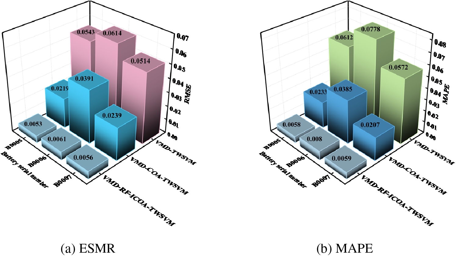
Figure 8: Evaluation indicator results (T = 30%)

Fig. 9 displays the SOH prediction results and absolute errors of three LIBs under the condition of T = 50%. As the number of training samples increases, the prediction performance of each model improves, and the error fluctuations slightly decrease. The VMD-RF-ICOA-TWSVM model continues to demonstrate the best accuracy in predicting the degradation trend of SOH. It also exhibits excellent adaptability to fluctuations in battery capacity regeneration and other variables. Fig. 10 presents the evaluation metrics for the model predictions at T = 50%. Upon analyzing these metrics, it is evident that the RMSE and MAPE of each model have improved compared to the training set at T = 30%. The VMD-RF-ICOA-TWSVM model achieves the most optimal evaluation metrics. For instance, taking B0005 as an example, the RMSE of the lithium battery is reduced to 0.0036, which represents a 32.09% improvement over the predictions at T = 30%, and the MAPE is reduced to 0.0036, indicating a 37.93% improvement over the predictions at T = 30%. These results underscore the excellent predictive capability of VMD-RF-ICOA-TWSVM across different starting points. Moreover, with a larger sample size in the training set, the predictive performance improves further, highlighting the model’s robust long-term predictive ability. Overall, the model demonstrates accurate and resilient performance in its predictions.

Figure 9: Prediction curve and absolute error (T = 50%)

Figure 10: Evaluation indicator results (T = 50%)

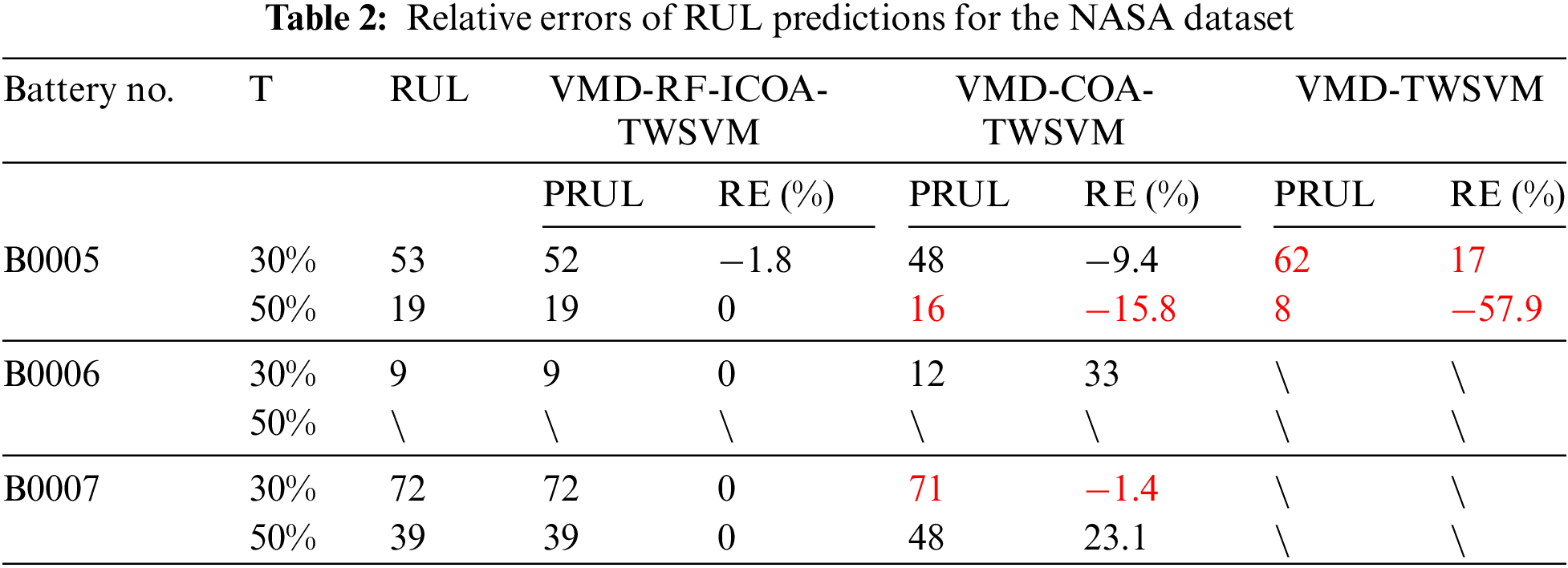
Table 2 presents the relative errors of RUL prediction for the NASA dataset. An absence of values indicates that the model did not predict the failure threshold. Red font highlights instances where the model’s predictions fluctuated near the failure threshold during the prediction process, indicating reduced stability. The VMD-TWSVM model predicted failure with relative errors of 18 and 19 in two results, reflecting unsatisfactory performance. The VMD-COA-TWSVM model produced prediction results but exhibited large relative errors that fluctuated near the failure threshold, rendering it unstable for capturing the RUL of LIBs. In contrast, the VMD-RF-ICOA-TWSVM model achieved the lowest relative errors for RUL prediction, except for B0005 at T = 30%, which had an error of −1.8%. However, all other errors were 0, ensuring that LIBs were neither underutilized nor overutilized.

The prediction results and absolute errors of different models for the CALCE dataset are depicted in Figs. 11 and 12, while the evaluation indices are presented in Table 3. At T = 30%, the maximum absolute error for VMD-RF-ICOA-TWSVM across all three LIBs (CS2-33, CS2-34, and CS2-36) does not exceed 0.018, with a maximum RMSE of 0.007 and a MAPE below 0.0082. At T = 50%, the maximum absolute error remains below 0.0169, with a maximum RMSE of 0.006 and a MAPE below 0.0077. At T = 50%, the maximum absolute error remains below 0.0169, with a maximum RMSE of 0.006 and a MAPE below 0.0077. Whether at T = 30% or T = 50%, the evaluation indices of VMD-RF-ICOA-TWSVM demonstrate optimal performance compared to other models, underscoring the excellent robustness and generalization capabilities of the model proposed in this study.

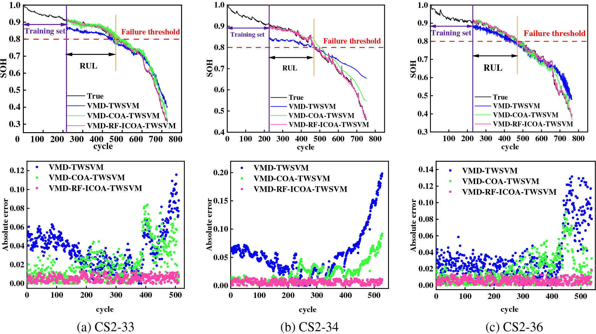
Figure 11: Prediction curve and absolute error (T = 30%)

Figure 12: Prediction curve and absolute error (T = 50%)

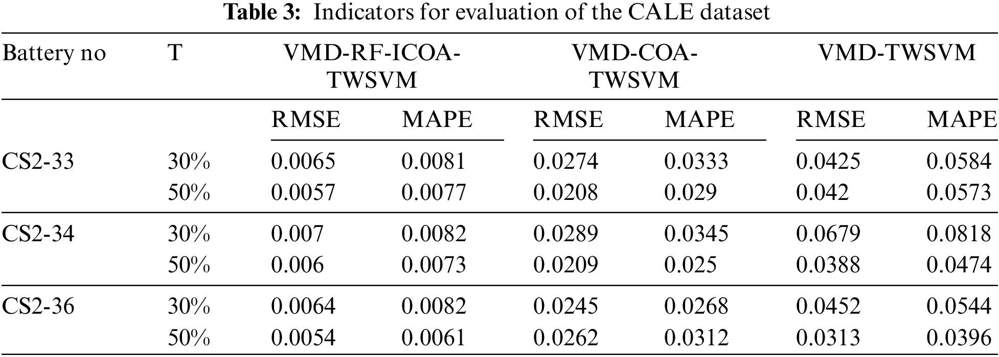
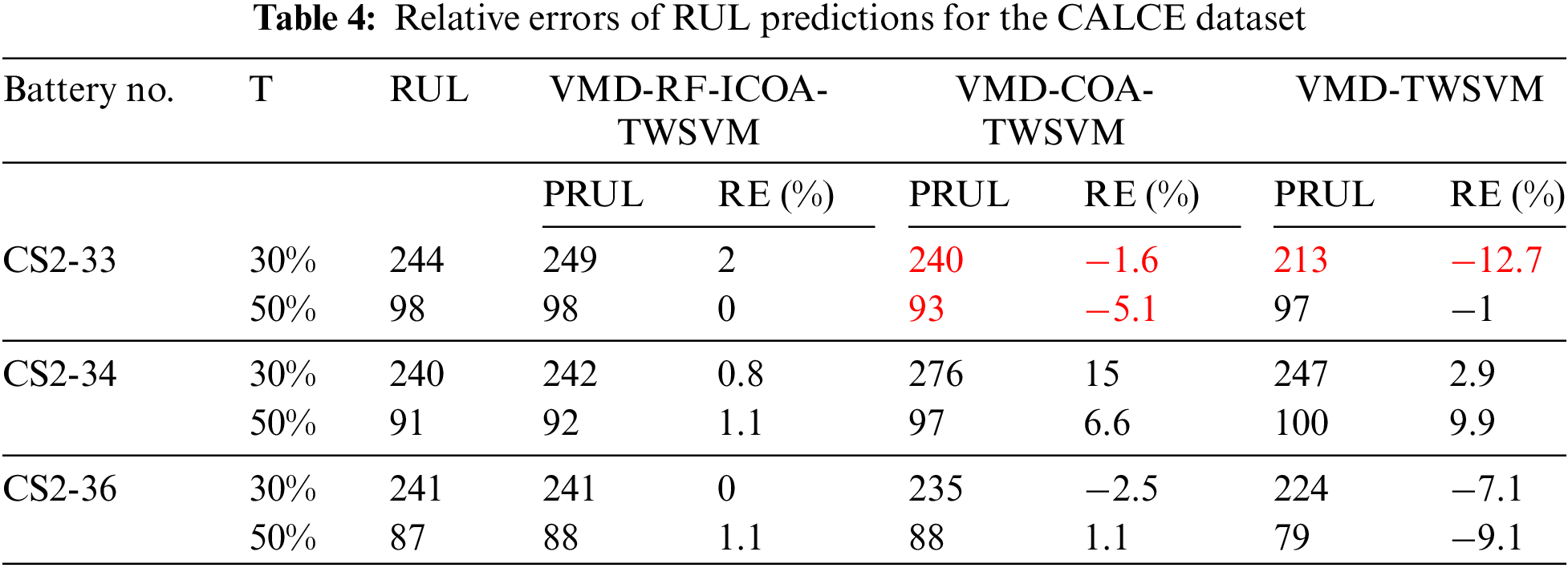
Table 4 presents the relative errors of RUL prediction for the CALCE dataset. It is observed that both VMD-COA-TWSVM and VMD-TWSVM exhibit fluctuations around the failure threshold during the prediction process. The RUL prediction errors for these models range from −5.1% to 15% and from −12.7% to 9%, respectively. In contrast, the RUL relative error of VMD-RF-ICOA-TWSVM falls within the range of 0% to 2%, the lowest among all models. This stable performance indicates that the model maintains accurate RUL predictions across batteries with varying lifespans and operating conditions.

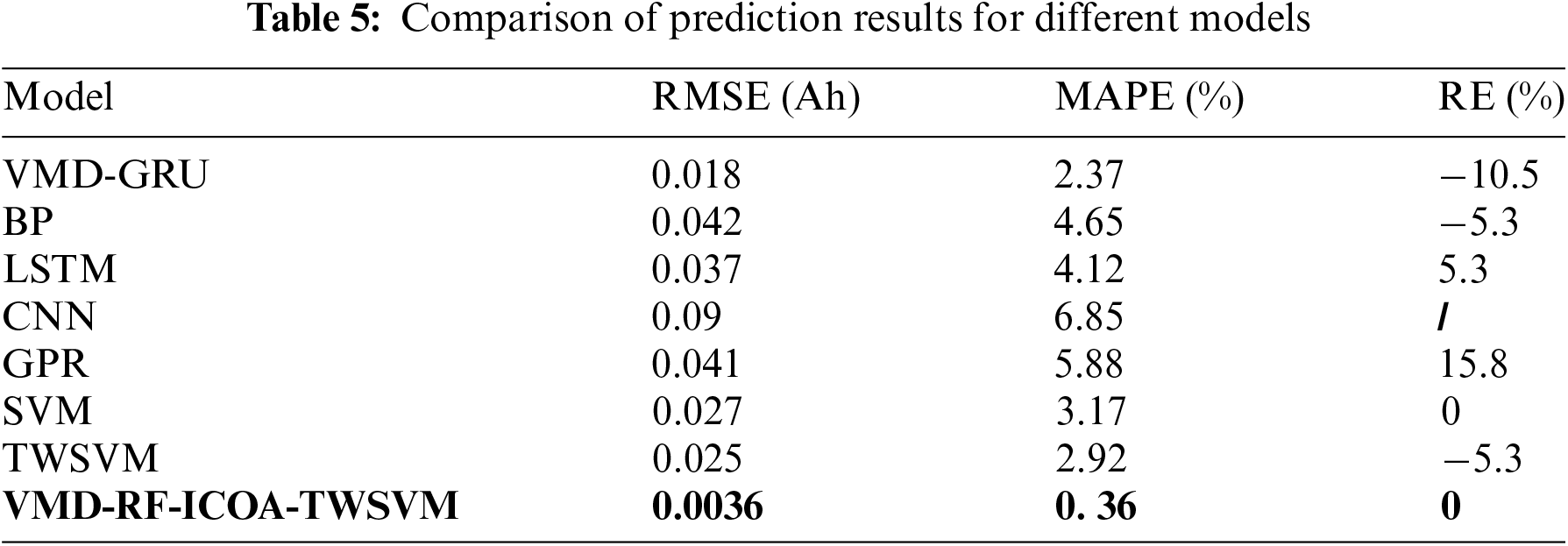
The proposed method is further compared with other models on the B0005 dataset, as shown in Table 5. Compared to TWSVM, the error metrics of the prediction results processed by the VMD-RF algorithm and ICOA algorithm significantly decrease, indicating an effective capture of the battery degradation trend and the ability to track sudden changes encountered during the battery aging process. Compared to other methods, VMD-RF-ICOA-TWSVM substantially outperforms other comparative models, demonstrating excellent predictive accuracy.

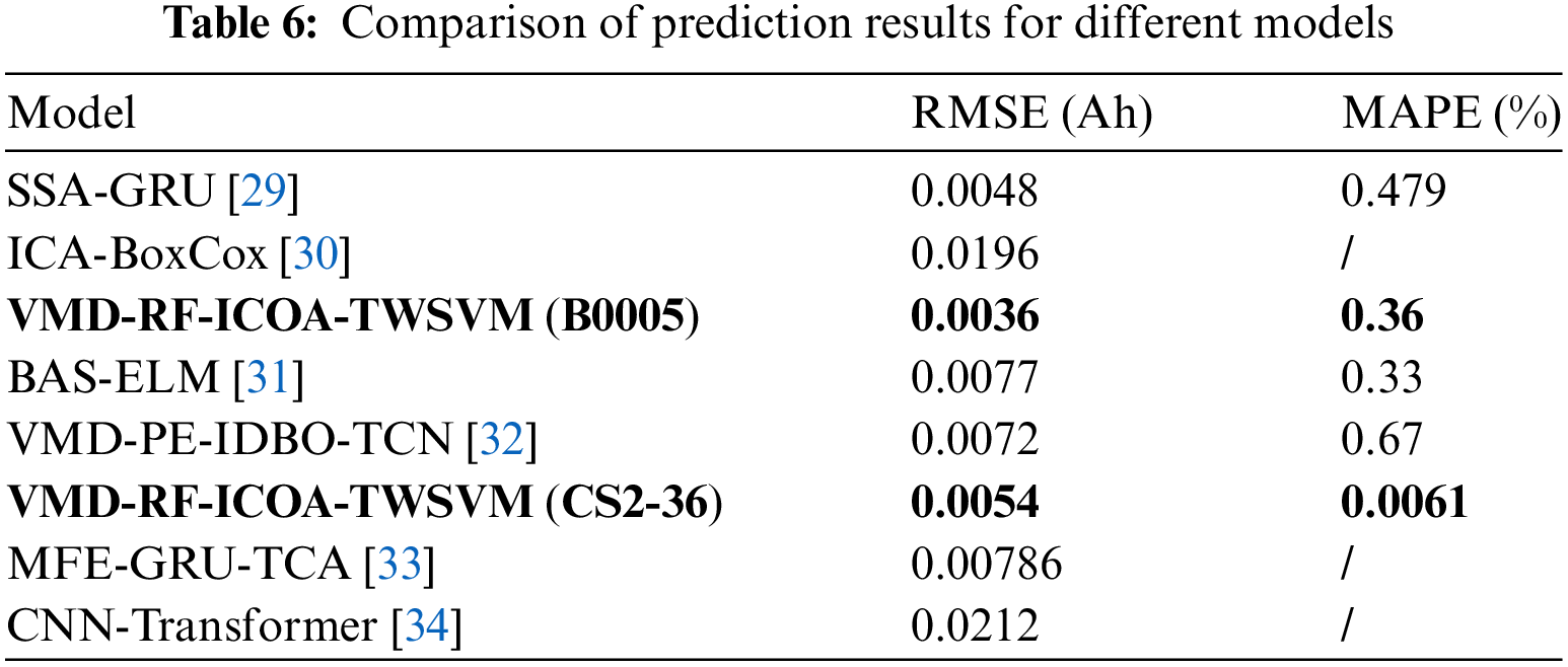
This study compares and analyzes recent literature. References [29,30] proposed a GRU-based method using current decay and a lithium-ion SOH estimation method based on incremental capacity analysis and Box-Cox transformation, respectively. References [31,32] simulated models using the NASA dataset, with the B0005 battery as an example, while References [33,34] based their simulations on the CALCE dataset, using the CS2-36 battery model. The prediction results are summarized in Table 6. The results show that the method proposed in this study outperforms the methods in [29,30] in both RMSE and MAPE. For the B0005 dataset, the BAS-ELM model performs slightly better in MAPE than the VMD-RF-ICOA-TWSVM model, but its RMSE is significantly higher, indicating that BAS-ELM may produce more outliers in predictions. When using the CS2-36 dataset, the proposed model continues to demonstrate strong performance compared to the MFE-GRU-TCA and CNN-Transformer models.

5  Conclusion

Accurate prediction of SOH and RUL is crucial for the safe use of LIBs. In this paper, HI is extracted by charging time, and VMD-RF is used as data processing to deal with the time series joint estimation framework of SOH and RUL based on improved TWSVM, and the specific conclusions are as follows:

a)   The VMD and RF combined model decomposes HI into components with different scale characteristics and excludes unimportant components. This effectively reduces the influence of disturbing factors in LIBs data on prediction accuracy.

b)   The parameter optimization performance of the convolutional optimization algorithm can be effectively improved by generating the initial population through the good point set method and refining parameters using the differential evolution method.

c)   Compared to other methods, VMD-RF-ICOA-TWSVM demonstrates optimal evaluation indices for predicting SOH and RUL, and it achieves superior predictive efficacy across different LIBs.

In future research, VMD-RF-ICOA-TWSVM will consider external environmental factors such as temperature and humidity, and will also expand into online prediction.

Acknowledgement: The authors acknowledge the reviewers for providing valuable comments and helpful suggestions to improve the manuscript.

Funding Statement: This research was funded by the Pyramid Talent Training Project of Beijing University of Civil Engineering and Architecture under Grant GJZJ20220802.

Author Contributions: The authors confirm contribution to the paper as follows: Conceptualization, methodology, validation, data collection, writing—original draft and editing: Liyao Yang; Supervision, funding acquisition, review: Hongyan Ma; Methodology, writing––review and editing: Yingda Zhang; Review and editing: Wei He. All authors reviewed the results and approved the final version of the manuscript.

Availability of Data and Materials: The data that support the findings of this study are available from the corresponding author upon reasonable request.

Ethics Approval: Not applicable.

Conflicts of Interest: The authors declare no conflicts of interest to report regarding the present study.

References

1. H. Bashir, A. Yaqoob, I. Jawaid, W. Khalid, M. Y. Javed and W. Sultan, “A review of battery management system and modern state estimation approaches in lithiumion batteries for electric vehicle,” in Proc. ICECE, Lahore, Pakistan, Mar. 16–17, 2022, pp. 1–8. [Google Scholar]

2. K. Song, D. Hu, Y. Tong, and X. Yue, “Remaining life prediction of lithium-ion batteries based on health management: A review,” J. Energy Storage, vol. 57, Jan. 2023, Art. no. 106193. doi: 10.1016/j.est.2022.106193. [Google Scholar] [CrossRef]

3. Y. Toughzaoui et al., “State of health estimation and remaining useful life assessment of lithium-ion batteries: A comparative study,” J. Energy Storage, vol. 51, Jul. 2022, Art. no. 104520. doi: 10.1016/j.est.2022.104520. [Google Scholar] [CrossRef]

4. K. Luo, X. Chen, H. Zheng, and Z. Shi, “A review of deep learning approach to predicting the state of health and state of charge of lithium-ion batteries,” J. Energy Chem, vol. 74, pp. 159–173, Nov. 2022. doi: 10.1016/j.jechem.2022.06.049. [Google Scholar] [CrossRef]

5. F. Xia, K. Wang, and J. Chen, “State of health and remaining useful life prediction of lithium-ion batteries based on a disturbance-free incremental capacity and differential voltage analysis method,” J. Energy Storage, vol. 64, Aug. 2023, Art. no. 107161. doi: 10.1016/j.est.2023.107161. [Google Scholar] [CrossRef]

6. X. Y. Yao, G. Chen, L. Hu, and M. Pecht, “A multi-model feature fusion model for lithium-ion battery state of health prediction,” J. Energy Storage, vol. 56, Dec. 2022, Art. no. 106051. doi: 10.1016/j.est.2022.106051. [Google Scholar] [CrossRef]

7. K. S. Ng, C. S. Moo, Y. P. Chen, and Y. C. Hsieh, “Enhanced coulomb counting method for estimating state-of-charge and state-of-health of lithium-ion batteries,” Appl. Energy, vol. 86, pp. 1506–1511, Sep. 2009. doi: 10.1016/j.apenergy.2008.11.021. [Google Scholar] [CrossRef]

8. Z. Pang, K. Yang, Z. Song, P. Niu, G. Chen and J. Meng, “A new method for determining SOH of lithium batteries using the real-part ratio of EIS specific frequency impedance,” J. Energy Storage, vol. 72, Nov. 2023, Art. no. 108693. doi: 10.1016/j.est.2023.108693. [Google Scholar] [CrossRef]

9. P. Reshma and V. J. Manohar, “Collaborative evaluation of SoC, SoP and SoH of lithium-ion battery in an electric bus through improved remora optimization algorithm and dual adaptive Kalman filtering algorithm,” J. Energy Storage, vol. 68, no. 1, Sep. 2023, Art. no. 107573. doi: 10.1016/j.est.2023.107573. [Google Scholar] [CrossRef]

10. Y. Li et al., “A hybrid machine learning framework for joint SOC and SOH estimation of lithium-ion batteries assisted with fiber sensor measurements,” Appl. Energy, vol. 325, Nov. 2022, Art. no. 119787. doi: 10.1016/j.apenergy.2022.119787. [Google Scholar] [CrossRef]

11. H. Zhou, J. Huan, and Z. Yu, “Co-estimation of SOC and SOH for Li-ion battery based on MIEKPF-EKPF fusion algorithm,” Energy Rep., vol. 10, pp. 4420–4428, Nov. 2023. doi: 10.1016/j.egyr.2023.11.017. [Google Scholar] [CrossRef]

12. P. Guo, Z. Cheng, and L. Yang, “A data-driven remaining capacity estimation approach for lithium-ion batteries based on charging health feature extraction,” J. Power Sources, vol. 412, pp. 442–450, Feb. 2019. doi: 10.1016/j.jpowsour.2018.11.072. [Google Scholar] [CrossRef]

13. Y. Zheng, Y. Cui, X. Han, and M. Ouyang, “A capacity prediction framework for lithium-ion batteries using fusion prediction of empirical model and data-driven method,” Energy, vol. 237, Dec. 2021, Art. no. 121556. doi: 10.1016/j.energy.2021.121556. [Google Scholar] [CrossRef]

14. V. C. N. Van and D. T. Quang, “Estimation of SoH and internal resistances of Lithium ion battery based on LSTM network,” Int. J. Electrochem. Sci., vol. 18, no. 6, Jun. 2023, Art. no. 100166. doi: 10.1016/j.ijoes.2023.100166. [Google Scholar] [CrossRef]

15. L. Chen, H. Wang, B. Liu, Y. Wang, Y. Ding and H. Pan, “Battery state-of-health estimation based on a metabolic extreme learning machine combining degradation state model and error compensation,” Energy, vol. 215, 2021, Art. no. 119078. doi: 10.1016/j.energy.2020.119078. [Google Scholar] [CrossRef]

16. S. Peikun and W. Zhenpo, “Research of the relationship between Li-ion battery charge performance and SOH based on MIGA-Gpr method,” Energy Proc., vol. 88, pp. 608–613, Jun. 2016. doi: 10.1016/j.egypro.2016.06.086. [Google Scholar] [CrossRef]

17. W. Duan, S. Song, F. Xiao, Y. Chen, S. Peng and C. Song, “Battery SOH estimation and RUL prediction framework based on variable forgetting factor online sequential extreme learning machine and particle filter,” J. Energy Storage, vol. 65, Aug. 2023, Art. no. 107322. doi: 10.1016/j.est.2023.107322. [Google Scholar] [CrossRef]

18. H. Xu, L. Wu, S. Xiong, W. Li, A. Garg and L. Gao, “An improved CNN-LSTM model-based state-of-health estimation approach for lithium-ion batteries,” Energy, vol. 276, Aug. 2023, Art. no. 127585. doi: 10.1016/j.energy.2023.127585. [Google Scholar] [CrossRef]

19. C. Li et al., “State-of-health and remaining-useful-life estimations of lithium-ion battery based on temporal convolutional network-long short-term memory,” J. Energy Storage, vol. 74, Dec. 2023, Art. no. 109498. doi: 10.1016/j.est.2023.109498. [Google Scholar] [CrossRef]

20. Q. Zhao, X. Qin, H. Zhao, and W. Feng, “A novel prediction method based on the support vector regression for the remaining useful life of lithium-ion batteries,” Microelectron. Reliab., vol. 85, pp. 99–108, Jun. 2018. doi: 10.1016/j.microrel.2018.04.007. [Google Scholar] [CrossRef]

21. T. Qin, S. Zeng, and J. Guo, “Robust prognostics for state of health estimation of lithium-ion batteries based on an improved PSO-SVR model,” Microelectron. Reliab., vol. 55, no. 9–10, pp. 1280–1284, Aug.–Sep. 2015. doi: 10.1016/j.microrel.2015.06.133. [Google Scholar] [CrossRef]

22. J. Qiao, X. Liu, and Z. Chen, “Prediction of the remaining useful life of lithium-ion batteries based on empirical mode decomposition and deep neural networks,” IEEE Access, vol. 8, pp. 42760–42767, Mar. 2020. doi: 10.1109/ACCESS.2020.2977429. [Google Scholar] [CrossRef]

23. G. Ding and H. Chen, “A RUL prediction method for lithium-ion batteries based on improved singular spectrum analysis and CSA-KELM,” Microelectron. Reliab., vol. 144, May 2023, Art. no. 114975. doi: 10.1016/j.microrel.2023.114975. [Google Scholar] [CrossRef]

24. S. Wang, H. Ma, Y. Zhang, S. Li, and W. He, “Remaining useful life prediction method of lithium-ion batteries is based on variational modal decomposition and deep learning integrated approach,” Energy, vol. 282, Nov. 2023, Art. no. 128984. doi: 10.1016/j.energy.2023.128984. [Google Scholar] [CrossRef]

25. K. W. Chen, S. Wei, and J. Zhang, “Intelligent optimization algorithm based on two-dimensional convolutional operations,” J. Armoured Corps, vol. 2, no. 1, pp. 102–108, 2023. doi: 10.3969/j.issn.20970986.2023.01.024. [Google Scholar] [CrossRef]

26. H. Que et al., “Study of denoising in the electricity anti-stealing detection based on VMD-WTD combination,” Energy Eng., vol. 119, no. 4, pp. 1453–1466, 2022. doi: 10.32604/ee.2022.018448. [Google Scholar] [CrossRef]

27. G. Wang, L. Sun, A. Wang, J. Jiao, and J. Xie, “Lithium battery remaining useful life prediction using VMD fusion with attention mechanism and TCN,” J. Energy Storage, vol. 93, Jul. 2024, Art. no. 112330. doi: 10.1016/j.est.2024.112330. [Google Scholar] [CrossRef]

28. Q. Qin, Y. Li, Y. Mi, J. Shen, K. Wu and Z. Wang, “Detecting XSS with random forest and multi-channel feature extraction,” Comput. Mater. Contin., vol. 80, no. 1, pp. 843–874, Jul. 2024. doi: 10.32604/cmc.2024.051769. [Google Scholar] [CrossRef]

29. C. Zhang et al., “Battery SOH estimation method based on gradual decreasing current, double correlation analysis and GRU,” Green Energy Intell. Transp., vol. 2, Oct. 2023, Art. no. 100108. doi: 10.1016/j.geits.2023.100108. [Google Scholar] [CrossRef]

30. J. Zhang, P. Wang, and Z. Cheng, “SOH estimation method for lithium-ion batteries based on ICA and Box-Cox transform,” J. Power Syst. Autom., vol. 34, pp. 9–15, 2022. doi: 10.19635/j.cnki.csu-epsa.000824. [Google Scholar] [CrossRef]

31. X. Hou et al., “The state of health prediction of Li-ion batteries based on an improved extreme learning machine,” J. Energy Storage, vol. 70, Oct. 2023, Art. no. 108044. doi: 10.1016/j.est.2023.108044. [Google Scholar] [CrossRef]

32. J. Fu, C. Wu, J. Wang, M. M.Haque, L. Geng and J. Meng, “Lithium-ion battery SOH prediction based on VMD-PE and improved DBO optimized temporal convolutional network model,” J. Energy Storage, vol. 87, May 2024, Art. no. 111392. doi: 10.1016/j.est.2024.111392. [Google Scholar] [CrossRef]

33. X. Wang, K. Dai, M. Hu, and N. Ni, “Lithium-ion battery health state and remaining useful life prediction based on hybrid model MFE-GRU-TCA,” J. Energy Storage, vol. 95, Aug. 2024, Art. no. 112442. doi: 10.1016/j.est.2024.112442. [Google Scholar] [CrossRef]

34. Z. Yuan, T. Tian, F. Hao, G. Li, R. Tang and X. Liu, “A hybrid neural network based on variational mode decomposition denoising for predicting state-of-health of lithium-ion batteries,” J. Power Sources, vol. 609, Jul. 2024, Art. no. 234697. doi: 10.1016/j.jpowsour.2024.234697. [Google Scholar] [CrossRef]