 Open Access
ARTICLE
Remaining Life Prediction Method for Photovoltaic Modules Based on Two-Stage Wiener Process
School of Electrical Engineering and Information Engineering, Lanzhou University of Technology, Lanzhou, 730050, China
* Corresponding Author: Jie Lin. Email:
Energy Engineering 2025, 122(1), 331-347. https://doi.org/10.32604/ee.2024.055611
Received 02 July 2024; Accepted 21 October 2024; Issue published 27 December 2024
Abstract
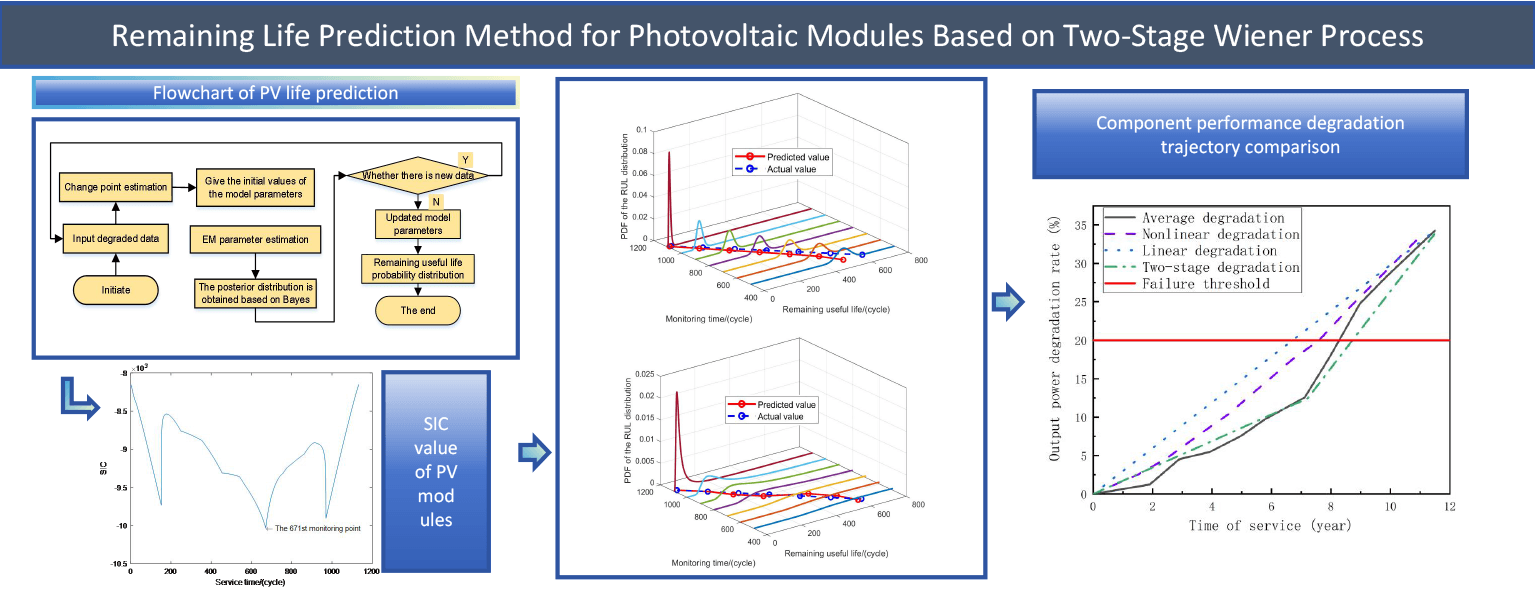
Photovoltaic (PV) modules, as essential components of solar power generation systems, significantly influence unit power generation costs. The service life of these modules directly affects these costs. Over time, the performance of PV modules gradually declines due to internal degradation and external environmental factors. This cumulative degradation impacts the overall reliability of photovoltaic power generation. This study addresses the complex degradation process of PV modules by developing a two-stage Wiener process model. This approach accounts for the distinct phases of degradation resulting from module aging and environmental influences. A power degradation model based on the two-stage Wiener process is constructed to describe individual differences in module degradation processes. To estimate the model parameters, a combination of the Expectation-Maximization (EM) algorithm and the Bayesian method is employed. Furthermore, the Schwarz Information Criterion (SIC) is utilized to identify critical change points in PV module degradation trajectories. To validate the universality and effectiveness of the proposed method, a comparative analysis is conducted against other established life prediction techniques for PV modules.Graphic Abstract
Keywords
Nomenclature
| Probability density function. | |
| RUL | Remaining useful life. |
| e.g., | |
| RUL at inspection time | |
| Time of the changing point. | |
| Degradation state at the changing point. | |
| Threshold of | |
| PDF of the lifetime. | |
| PDF of the RUL. | |
| Drift coefficient at the ith phase. | |
| Diffusion coefficient at the ith phase. | |
| PDF of the standard normal distribution. | |
| Cumulative distribution function of the standard normal distribution. | |
| Standard variances of | |
| Means of | |
The PV module, a critical component of a PV power generation system, accounts for approximately 60% of the total cost. Ideally, the service life of a PV module should exceed 25 years [1–4]. However, in practice, environmental factors and external stresses often lead to a shorter lifespan than expected [5,6]. Furthermore, the extended service life of PV modules presents challenges in collecting degraded power data. Therefore, it is essential to investigate the degradation characteristics of PV modules using stochastic degradation models. These models facilitate the estimation of remaining service life and the development of appropriate maintenance strategies.
Currently, there are two main methods for predicting PV module life: failure mechanism-based and data-driven [7,8]. Failure mechanism-based PV module life prediction methods primarily forecast PV module life by quantifying the relationship between environmental pressure and output power, without requiring performance degradation monitoring data. However, these methods necessitate prior knowledge of the physical mechanisms underlying the degradation process and have inherent limitations. Kaaya et al. [9] proposed a PV prediction model based on local climate, which offers the advantage of applicability after a small performance degradation and can improve prediction accuracy with fewer input variables. A generalized model was proposed in [10] to quantify the impact of integrated climate loads and predict the degradation rate of single crystal components in different climates. Liu et al. [11] propose a semi-parametric framework for on-site photovoltaic systems with periodic attenuation signals to predict the remaining life of photovoltaic modules in dynamic environments. In contrast to failure mechanism model-based approaches, data-driven methods do not rely on specific physical or expert knowledge. These methods can uncover mathematical relationships between input data and targets to reveal hidden correlations and predict the remaining lifetime based on model parameters. Data-driven methods for PV module life prediction depend on the accumulation of historical monitoring data. Kaaya et al. [12] propose a hybrid drive model based on data algorithm drive and physical drive to obtain long-term reliable estimates of photovoltaic modules. Because the amount of PV module degradation exhibits continuous degradation characteristics over time, there are three main continuous-state degradation models: the gamma process, Wiener process, and inverse Gaussian process [13]. Park et al. [14], addressing the uncertainty and volatility in the degradation process of photovoltaic modules, compare three different life estimation methods and identify the prediction based on the gamma process model as the most applicable. Karakaya et al. [15] predict the life of inverters in photovoltaic modules using a data-driven approach, which is primarily divided into two stages: feature extraction and classification. Gamma and inverse Gaussian process models typically describe monotonic degradation processes [16–18] and have certain limitations in describing PV module degradation models. The Wiener process, originating from Brownian motion with a linear drift term, can describe the non-monotonic degradation process, which is favorable for the estimation of model parameters [19,20]. Wei et al. [21] propose a PV prediction model based on the Wiener process, which also considers individual differences, and models the degradation of photovoltaic modules to predict life. In [22], the life cycle of PV modules is obtained by combining a Wiener process with an acceleration time model. However, in practice, the deterioration of PV modules is caused by factors such as the natural environment, product aging, and external shocks, and a two-stage degradation phenomenon exists [20]. Nevertheless, current research on PV module life prediction does not consider the two-stage degradation of PV modules.
In summary, the traditional Wiener process model struggles to accurately depict the deterioration process of PV modules in the presence of variable points. To address this challenge, this study employs a two-stage Wiener degradation model to characterize the degradation process. Furthermore, Bayesian inference and the EM algorithm are introduced for the estimation of the model parameters. Finally, the feasibility and validity of the proposed method were verified by comprehensive simulation and practical case analysis.
The principal contributions of the proposed model are as follows:
1) A novel two-stage degradation model for PV modules has been developed, incorporating a random parameter to account for sample variability. The analytical expression of the remaining useful life (RUL) distribution of the two-stage system in the first arrival time is derived, enabling online real-time RUL estimation. Compared to single-stage models, the proposed model demonstrates superior alignment with engineering practices and exhibits enhanced accuracy.
2) The EM algorithm and Bayesian algorithm are proposed in this study. The life prediction results derived from these algorithms provide a robust theoretical foundation for optimizing the operation and maintenance cycle of PV modules.
2 PV Module Performance Degradation Model
The failure rate of PV modules changes over time due to the impact of environmental conditions, external stresses, and other random factors, which can be described by the bathtub curve, consisting of three distinct phases. The initial phase exhibits a higher failure rate, primarily attributed to defects in the PV module manufacturing process. During the second phase, the failure rate decreases as defective modules are eliminated, although random failures still occur due to environmental factors and external stresses. The third phase is characterized by an increase in the failure rate caused by fatigue, aging, and depletion of the PV modules resulting from prolonged usage [23]. Since the initial degradation is assumed to be zero in the performance degradation process of PV modules, most decay curves exhibit two stages. The Wiener process effectively simulates the non-monotonic deterioration process, offering robust data fitting capabilities and mathematical properties [24]. Due to the degradation process of PV modules, two distinct stages of degradation trajectories are observed. In summary, this study proposes a PV module life prediction method based on a two-stage degradation trajectory.
(1) The performance degradation curve of PV modules exhibits a distinct two-stage pattern. Although the precise location of the change point remains undetermined, engineers and technicians possess the ability to identify the periods preceding and following this transition [25].
(2) The degradation process at each stage conforms to an independent linear Wiener process, which can be expressed as:
In this equation,
(3) The lifetime
The remaining lifetime
Based on the aforementioned assumptions, the following two-stage Wiener degradation model can be developed:
where
3 Remaining Useful Life Prediction
If the drift coefficients
(1) when
(2) when
We define:
Eq. (14) can be derived from Eqs. (5)–(13).
(3) when
4 Model Parameters and Updates
4.1 Hyperparameter Estimation Based on EM Algorithm
In practical engineering, the same type of historical degradation data is frequently utilized as prior information for equipment. In this section, the EM algorithm’s parameter estimation is employed to estimate the prior information. Consider a total of
Let
where
where
where
After maximizing the conditional expectation and employing the EM algorithm, the result of the
4.2 Parameter Updates Based on Bayesian Methods
This section aims to integrate the prior information from the previous section with the current operational data for PV module degradation equipment in a degradation process. The initial degradation stage of the PV module occurs when
Style:
Given that
In contrast, the second degradation stage of the PV module degradation occurs when
Schwartz proposed the SIC in 1978 to determine whether a model has a variation-point problem. The SIC offers a straightforward method for estimating the change point in PV module degradation, demonstrating effective detection capabilities [32]. The SIC is defined as:
where
To determine the change point locations using the SIC, the following hypotheses are proposed:
Null hypothesis (H0): All parameters are equal, indicating the absence of change points in the model.
Alternative hypothesis (H1): There is a variable point
Based on Eq. (35), the SIC value under H0 is:
The SIC(k) value under the H1 is:
When
In conclusion, the remaining life prediction process of the PV module can be derived from the two-stage Wiener process, which involves variable point estimation and parameter updating, as depicted in Fig. 1.
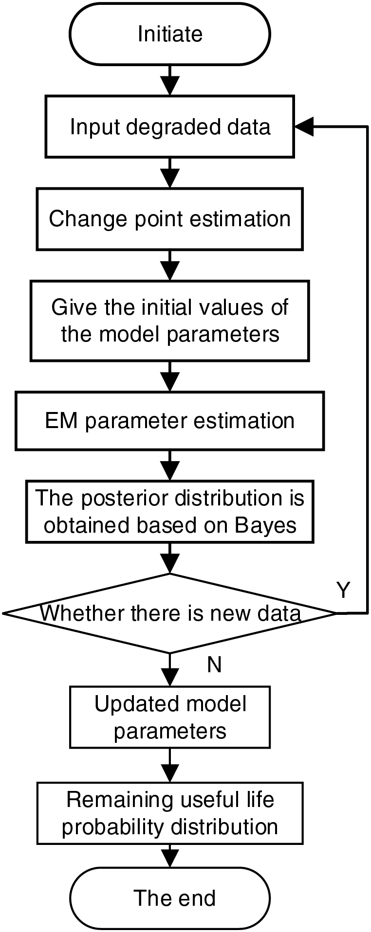
Figure 1: Flowchart of PV life prediction
5 Single-Stage Wiener Degeneracy Model
Based on the single-stage Wiener process model, the life
At
In conjunction with Eq. (1), the PDF can be expressed as:
Let
Upon deriving the posterior distribution, the EM algorithm is employed to calculate the positional parameter vector
By substituting the parameter estimates into Eq. (43), the remaining life prediction model is obtained.
To validate the feasibility of the proposed method, a comparative case study was conducted using data from Reference [33]. The study compared the life prediction results obtained from the single-stage Wiener process modeling approach with those derived from the methodology presented in this paper.
To facilitate analysis, the output power degradation data for the S73L47 module between 12 years of service was processed based on cases in the literature and divided into 1200 cycles, as depicted in Fig. 2.
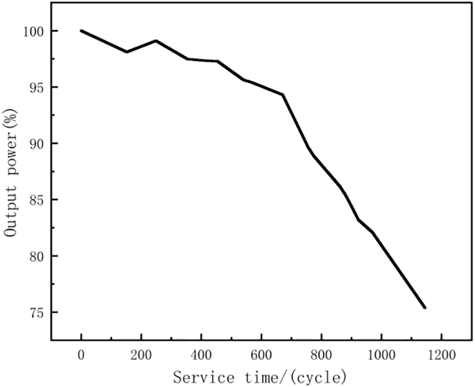
Figure 2: Degradation data
Adhering to the S73L47 power degradation model, the obsolescence threshold was established at 80% of the initial output power
Initially, the degradation model was monitored for change points using the SIC to determine the change point location; the corresponding trend of the SIC value is shown in Fig. 3. According to the SIC criterion, there is a change point in the degradation of the PV module and
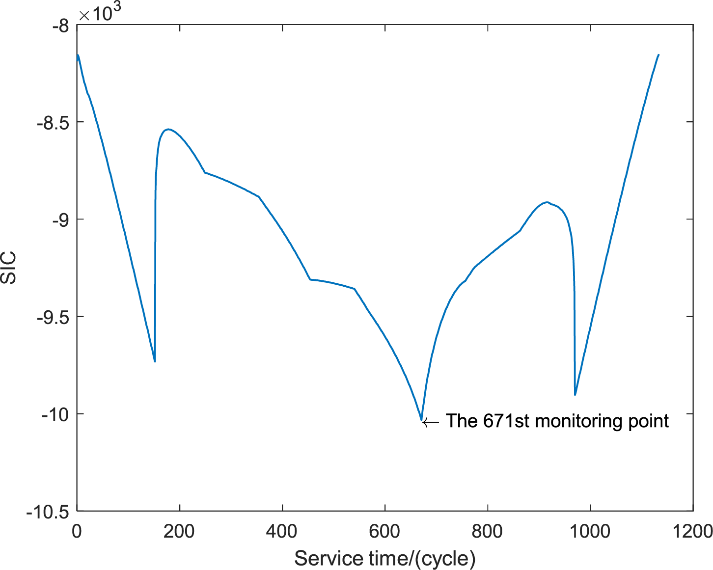
Figure 3: SIC value of PV modules
The resulting parameter estimates are
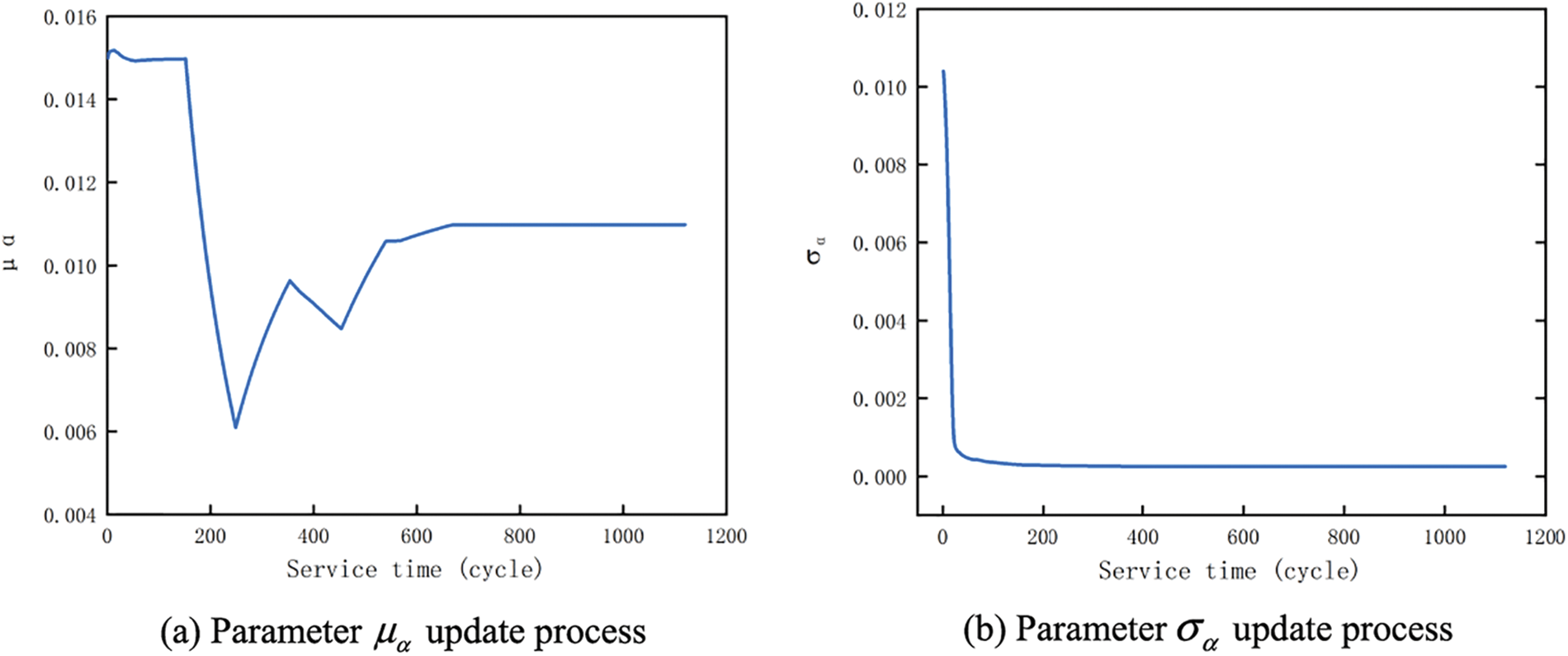
Figure 4: The first stage of model parameter updating
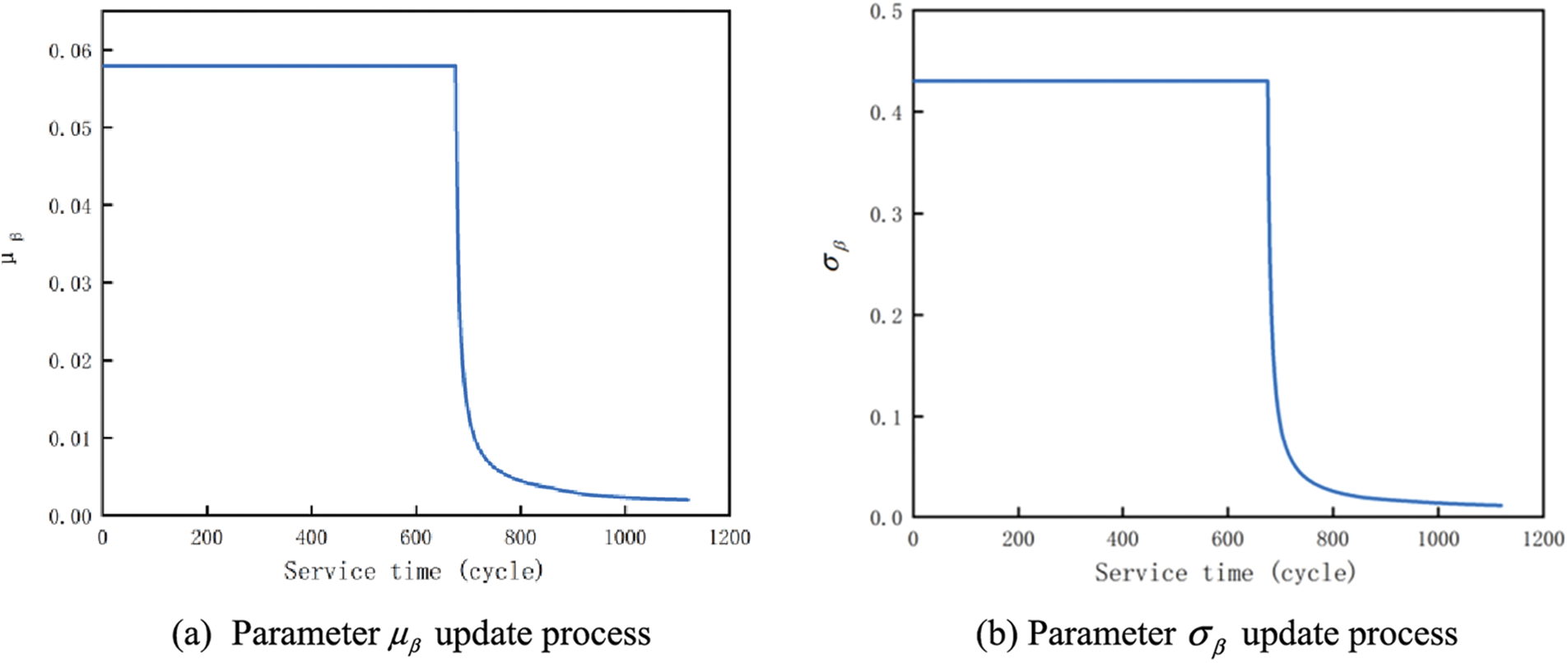
Figure 5: The second stage of model parameter updating
Figs. 6 and 7 illustrate the life prediction results and relative error values for the S73L47 PV module. The proposed model exhibits notably superior prediction accuracy compared to the single-stage model as the duration increases. This improved performance stems from the single-stage model’s inability to effectively capture the degradation trajectory of PV modules in the presence of a change point. By accurately modeling the degradation trajectory, the proposed approach achieves enhanced prediction accuracy.
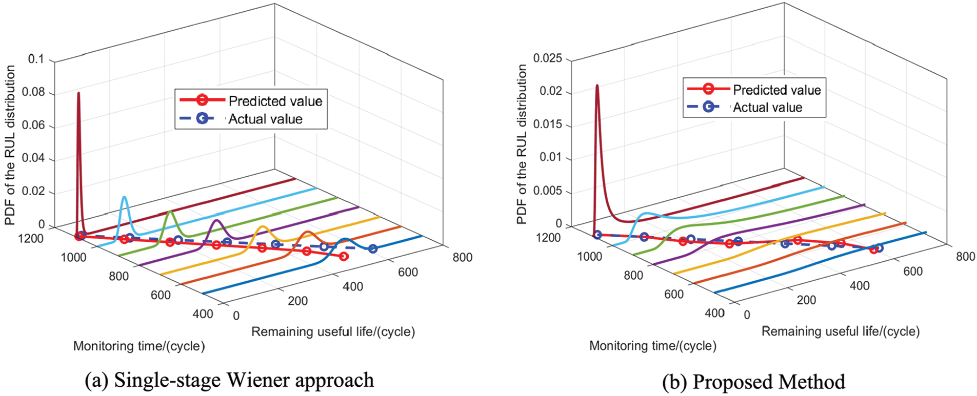
Figure 6: Prediction results of different methods
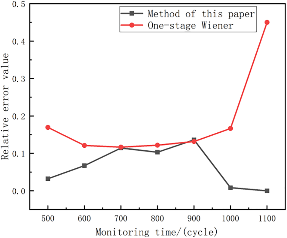
Figure 7: Relative value curves of remaining life prediction results
To illustrate the proposed model’s suitability for analyzing PV module degradation processes, this study compares and examines average degradation curves from four PV module groups, as depicted in Fig. 8. The degradation data is sourced from the literature [33], ensuring the analysis is grounded in established research.
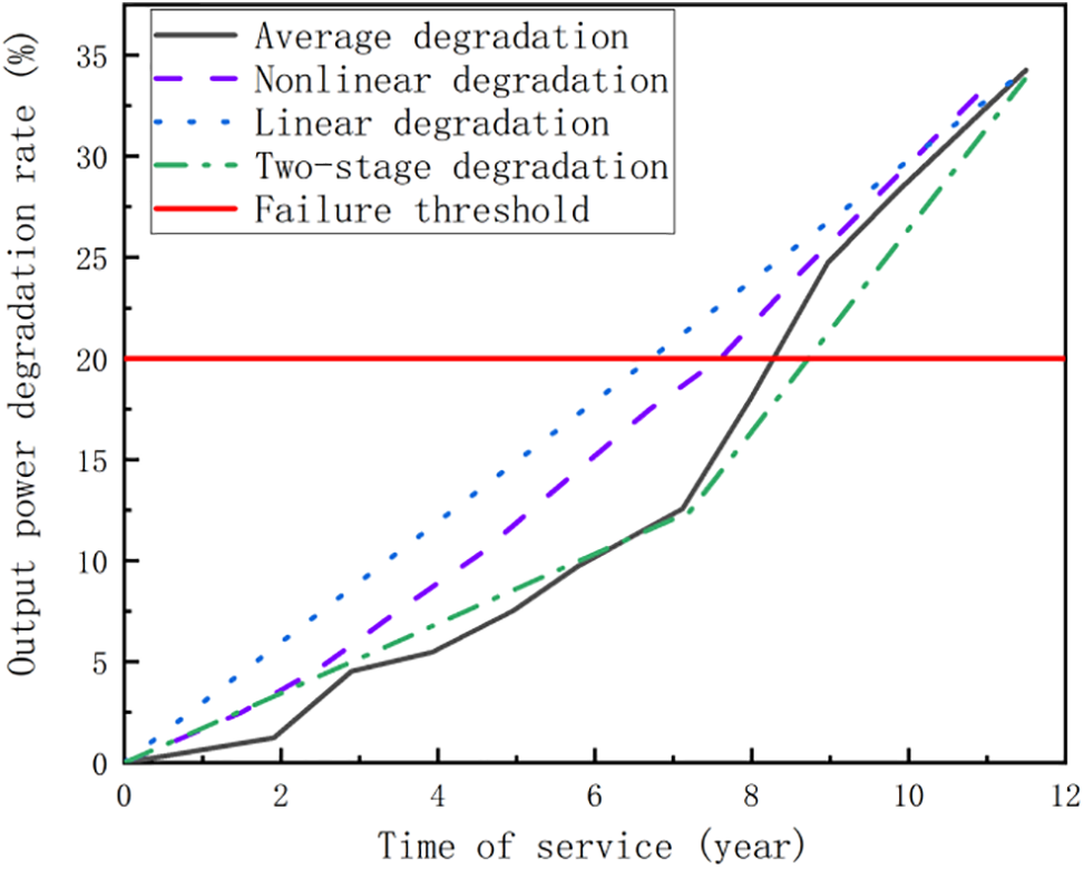
Figure 8: Component performance degradation trajectory comparison
Fig. 8 illustrates that the two-stage degradation model accurately fits the PV module degradation curve. Furthermore, as demonstrated in Table 1, the two-stage Wiener process model generates smaller lifetime prediction errors in comparison to both linear and nonlinear degradation models.

In light of the two-stage degradation phenomenon observed in PV modules, which is influenced by natural conditions and other stochastic factors in real-world scenarios, as well as the inter-individual variability of degradation rates and critical change points in PV systems, this study proposes a novel two-stage process for predicting PV module lifetimes. This approach addresses the complex nature of PV module degradation more comprehensively than existing methods. To enhance the model’s accuracy and robustness, a combination of the EM algorithm and Bayesian inference methods was employed for estimating model parameters and hyperparameters. Additionally, the SIC was utilized to detect the critical change point in the degradation curve, allowing for a more precise identification of transitions between degradation stages. Comparative analyses demonstrate that the proposed method achieves higher real-time accuracy in predicting the remaining life of PV modules compared to existing techniques. This improved predictive capability is particularly beneficial for developing more effective and efficient maintenance strategies for PV modules, ultimately contributing to the optimization of solar energy systems’ performance and longevity.
Although this study focuses on two-stage random degradation equipment with accessible degradation data, it is crucial to recognize that large, complex equipment may display multiple working conditions or state-switching phenomena due to environmental factors and varying work tasks, leading to multi-stage scenarios. Future research could extend the modeling of degradation and prediction of RUL to encompass multi-state and multi-stage complex random systems, while also addressing related maintenance decision challenges.
Acknowledgement: None.
Funding Statement: This work was supported by the National Natural Science Foundation of China (51767017), the Basic Research Innovation Group Project of Gansu Province (18JR3RA133), the Industrial Support and Guidance Project of Universities in Gansu Province (2022CYZC-22).
Author Contributions: The authors confirm contribution to the paper as follows: study conception and design: Jie Lin, Hongchi Shen; data collection: Hongchi Shen, Yan Wu; analysis and interpretation of results: Tingting Pei, Jie Lin; draft manuscript preparation: Yan Wu, Tingting Pei. All authors reviewed the results and approved the final version of the manuscript.
Availability of Data and Materials: Data supporting this study are included within the article.
Ethics Approval: Not applicable.
Conflicts of Interest: The authors declare that they have no conflicts of interest to report regarding the present study.
References
1. A. Omazic et al., “Relation between degradation of polymeric components in crystalline silicon PV module and climatic conditions: A literature review,” Sol. Energy Mater. Sol. Cells, vol. 192, no. 1, pp. 123–133, Apr. 2019. doi: 10.1016/j.solmat.2018.12.027. [Google Scholar] [CrossRef]
2. M. A. Munoz, M. C. Alonso-García, N. Vela, and F. Chenlo, “Early degradation of silicon PV modules and guaranty conditions,” Sol. Energy, vol. 85, no. 9, pp. 2264–2274, Sep. 2011. doi: 10.1016/j.solener.2011.06.011. [Google Scholar] [CrossRef]
3. H. Han et al., “Degradation analysis of crystalline silicon photovoltaic modules exposed over 30 years in hot-humid climate in China,” Sol. Energy, vol. 170, no. 1, pp. 510–519, Aug. 2018. doi: 10.1016/j.solener.2018.05.027. [Google Scholar] [CrossRef]
4. D. C. Jordan, S. R. Kurtz, K. VanSant, and J. Newmiller, “Compendium of photovoltaic degradation rates,” Prog. Photovolt., vol. 24, no. 1, pp. 978–989, Feb. 2016. doi: 10.1002/pip.2744. [Google Scholar] [CrossRef]
5. S. Voswinckel, T. Mikolajick, and V. Wesselak, “Influence of the active leakage current pathway on the potential induced degradation of CIGS thin film solar modules,” Sol. Energy, vol. 197, no. 1, pp. 455–461, Feb. 2020. doi: 10.1016/j.solener.2019.12.078. [Google Scholar] [CrossRef]
6. M. Halwachs et al., “Statistical evaluation of PV system performance and failure data among different climate zones,” Renew. Energy, vol. 139, no. 1, pp. 1040–1060, Aug. 2019. doi: 10.1016/j.renene.2019.02.135. [Google Scholar] [CrossRef]
7. I. Kaaya, J. Ascencio-Vásquez, K. -A. Weiss, and M. Topič, “Assessment of uncertainties and variations in PV modules degradation rates and lifetime predictions using physical models,” Sol. Energy, vol. 218, no. 1, pp. 354–367, Apr. 2021. doi: 10.1016/j.solener.2021.01.071. [Google Scholar] [CrossRef]
8. L. Liao and F. Köttig, “Review of hybrid prognostics approaches for remaining useful life prediction of engineered systems, and an application to battery life prediction,” IEEE Trans. Reliab., vol. 63, no. 1, pp. 191–207, Mar. 2014. doi: 10.1109/TR.2014.2299152. [Google Scholar] [CrossRef]
9. I. Kaaya, S. Lindig, K. -A. Weiss, A. Virtuani, M. S. de Cardona Ortin and D. Moser, “Photovoltaic lifetime forecast model based on degradation patterns,” Prog. Photovolt., vol. 28, no. 10, pp. 979–992, Jul. 2020. doi: 10.1002/pip.3280. [Google Scholar] [CrossRef]
10. I. Kaaya, M. Koehl, A. P. Mehilli, S. de Cardona Mariano, and K. A. Weiss, “Modeling outdoor service lifetime prediction of PV modules: Effects of combined climatic stressors on PV Module power degradation,” IEEE J. Photovolt., vol. 9, no. 4, pp. 1105–1112, Jul. 2019. doi: 10.1109/JPHOTOV.2019.2916197. [Google Scholar] [CrossRef]
11. Q. Liu, Q. Hu, J. Zhou, D. Yu, and H. Mo, “Remaining useful life prediction of PV systems under dynamic environmental conditions,” IEEE J. Photovolt., vol. 13, no. 4, pp. 590–602, Jul. 2023. doi: 10.1109/JPHOTOV.2023.3272071. [Google Scholar] [CrossRef]
12. I. Kaaya and K. -A. Weiss, “Physical and data-driven hybrid model for outdoor lifetime prediction of PV modules,” presented at the 2020 47th IEEE Photovolt. Spec. Conf. (PVSCCalgary, AB, Canada, Jun. 15–Aug. 21, 2020. [Google Scholar]
13. Z. -S. Ye and M. Xie, “Stochastic modelling and analysis of degradation for highly reliable products,” Appl. Stoch. Models Bus. Ind., vol. 31, no. 1, pp. 16–23, Oct. 2014. doi: 10.1002/asmb.2063. [Google Scholar] [CrossRef]
14. S. -H. Park and J. -H. Kim, “Application of gamma process model to estimate the lifetime of photovoltaic modules,” Sol. Energy, vol. 147, no. 1, pp. 390–398, May 2017. doi: 10.1016/j.solener.2017.03.061. [Google Scholar] [CrossRef]
15. S. Karakaya et al., “Leveraging high-fidelity sensor data for inverter diagnostics: A data-driven model using high-temperature accelerated life testing data,” presented at the 2023 IEEE 50th Photovolt. Spec. Conf. (PVSCSan Juan, PR, USA, Jun. 11–16, 2023. [Google Scholar]
16. Q. Guan and X. Wei, “The statistical data-driven remaining useful life prediction—A review on the wiener process-based method,” presented at the 2023 Progn. Health Manag. Conf. (PHMParis, France, May 31–Jun. 02, 2023. [Google Scholar]
17. Z. Pan and N. Balakrishnan, “Reliability modeling of degradation of products with multiple performance characteristics based on gamma processes,” Reliab. Eng. Syst. Saf., vol. 96, no. 8, pp. 949–957, Aug. 2011. doi: 10.1016/j.ress.2011.03.014. [Google Scholar] [CrossRef]
18. H. X. Kou, Z. W. An, and Q. Ma, “Fatigue reliability assessment of wind turbine blades based on the performance degradation data,” (in Chinese), Acta Energiae Solaris Sinica, vol. 38, no. 11, pp. 3174–3179, Nov. 2017. [Google Scholar]
19. H. Wang, Y. Zhao, and X. Ma, “Remaining useful life prediction using a novel two-stage wiener process with stage correlation,” IEEE Access, vol. 6, no. 1, pp. 65227–65238, Oct. 2018. doi: 10.1109/ACCESS.2018.2877630. [Google Scholar] [CrossRef]
20. S. Mishra and O. A. Vanli, “Remaining useful life estimation with lamb-wave sensors based on wiener process and principal components regression,” J. Nondestr. Eval., vol. 35, no. 11, pp. 1–13, Dec. 2015. doi: 10.1007/s10921-015-0328-2. [Google Scholar] [CrossRef]
21. W. Chen, H. Lei, T. T. Pei, and X. B. Li, “Remaining life prediction method of photovoltaic modules based on degradation trajectory and Wiener model,,” (in Chinese), Acta Energy Sol. Sin., vol. 44, no. 44, pp. 175–181, Jul. 2023. [Google Scholar]
22. A. Charki, R. Laronde, and D. Bigaud, “Accelerated degradation testing of a photovoltaic module,” J. Photon. Energy, vol. 3, no. 1, Mar. 2013, Art. no. 33099. doi: 10.1117/1.JPE.3.033099. [Google Scholar] [CrossRef]
23. Y. Q. Yao, “Research on reliability modeling and condition-based maintenance strategy of two-phase degradation system,” M.S. thesis, Tianjin Univ., China, 2020. [Google Scholar]
24. Z. Zhang, X. Si, C. Hu, and Y. Lei, “Degradation data analysis and remaining useful life estimation: A review on Wiener-process-based methods,” Eur. J. Oper. Res., vol. 271, no. 3, pp. 775–796, Dec. 2018. doi: 10.1016/j.ejor.2018.02.033. [Google Scholar] [CrossRef]
25. P. Zhang, C. H. Hu, C. Bai, Y. Zhang, and J. X. Zhang, “Remaining useful life estimation method for two-phase degradation systems with random effects,” (in Chinese), China Meas. Test, vol. 45, no. 1, pp. 1–7, Jan. 2019. [Google Scholar]
26. M. -L. Ting Lee, and G. A. Whitmore, “Threshold regression for survival analysis: Modeling event times by a stochastic process reaching a boundary,” Stat. Sci., vol. 21, no. 4, pp. 501–513, Nov. 2006. doi: 10.1214/088342306000000330. [Google Scholar] [CrossRef]
27. J. -X. Zhang, C. -H. Hu, X. He, X. -S. Si, Y. Liu and D. -H. Zhou, “A Novel lifetime estimation method for two-phase degrading systems,” IEEE Trans. Reliab., vol. 68, no. 2, pp. 689–709, Jun. 2019. doi: 10.1109/TR.2018.2829844. [Google Scholar] [CrossRef]
28. X. -S. Si, W. Wang, C. -H. Hu, M. -Y. Chen, and D. -H. Zhou, “A Wiener-process-based degradation model with a recursive filter algorithm for remaining useful life estimation,” Mech. Syst. Signal Process., vol. 35, no. 1–2, pp. 219–237, Feb. 2013. doi: 10.1016/j.ymssp.2012.08.016. [Google Scholar] [CrossRef]
29. X. Y. Kou, B. Shuai, and W. C. Wang, “Analysis on operation fault of high-speed EMU based on Bayesian network,” (in Chinese), J. Saf. Sci. Technol., vol. 16, no. 4, pp. 63–69, Apr. 2020. doi: 10.11731/j.issn.1673-193x.2020.04.010. [Google Scholar] [CrossRef]
30. T. X. Xu, H. W. Wang, and X. Zhang, “Application of the EM algorithm to estimate hyper parameters of the random parameters of Wiener process,” (in Chinese), Syst. Eng. Electr., vol. 37, no. 3, pp. 707–712, Mar. 2015. doi: 10.3969/j.issn.1001-506X.2015.03.36. [Google Scholar] [CrossRef]
31. W. Wang, M. Carr, W. Xu, and K. Kobbacy, “A model for residual life prediction based on Brownian motion with an adaptive drift,” Microelectron. Reliab., vol. 51, no. 2, pp. 285–293, Feb. 2011. doi: 10.1016/j.microrel.2010.09.013. [Google Scholar] [CrossRef]
32. Q. Dong, J. F. Zheng, C. H. Hu, B. Li, and H. X. Mou, “Remaining useful life prognostic method based on two-stage adaptive wiener process,” (in Chinese), Acta Auto. Sin., vol. 48, no. 2, pp. 539–553, Feb. 2022. doi: 10.16383/j.aas.c210057. [Google Scholar] [CrossRef]
33. W. D. Liu, G. Wen, W. A. Yan, J. Luo, and X. H. Jiang, “Field lifetime assessment of photovoltaic modules based on degradation data-driven and nonlinear Gamma processes,” (in Chinese), Comput. Integr. Manuf. Syst., vol. 27, no. 12, pp. 3494–3502, Dec. 2021. [Google Scholar]
Cite This Article
 Copyright © 2025 The Author(s). Published by Tech Science Press.
This work is licensed under a Creative Commons Attribution 4.0 International License , which permits unrestricted use, distribution, and reproduction in any medium, provided the original work is properly cited.


 Submit a Paper
 Propose a Special lssue
 View Full Text
 Download PDF
 Downloads
 Citation Tools