A Fault Detection Method for Electric Vehicle Battery System Based on Bayesian Optimization SVDD Considering a Few Faulty Samples

1  Introduction

In the context of the world’s scarcity of kerosene resources and increasing environmental pollution, the application of new energy batteries is gradually showing up in front of people’s eyes and developing rapidly from the point of view of economic benefits, environmental protection awareness and lifestyle, especially the development of new energy electric vehicles (EVs) is the most rapid. The lithium-ion battery system is the key technology of new energy EVs because it has the advantages of high working voltage, high specific energy, small volume, light mass, long cycle life, low pollution, and so on. However, in real life, the failure mechanism generated by the battery system in a closed environment is very complex, and overcharging, over-discharging, and electrolyte leakage of the battery can lead to serious hazards such as battery bulging, smoke, and fire [1,2]. The external impact of the EVs, the limitations of the production process, and the harsh factors such as high and low temperatures may cause short circuits and thermal runaway, and even cause battery combustion, which seriously jeopardizes driving safety [3,4]. Therefore, in order to solve the early and minor faults of lithium-ion batteries as early as possible and to reduce the probability of danger, it is crucial to accurately detect faults in the battery system.

In recent years, fault detection of EVs batteries has been a very important research topic [5]. After reviewing the research and discussions of many scholars on the fault detection aspects of lithium-ion batteries, among the current research methods, model-based methods, knowledge-based methods, and data-driven methods are still the more advanced methods [6–8].

The model-based methods mainly include the parameter estimation method, state estimation method, parity space method, and structural analysis method [9]. The method is mainly based on establishing a clear physical model of the battery system, comparing the measurable signals with the model-generated signals to obtain the residual signals, and comparing the residual signals with the fault thresholds to determine whether the battery system has a fault. However, due to other factors such as the complex nonlinearity and time variability of the actual battery system, the above method is not very feasible to accurately model the battery and is difficult to apply in practice. The knowledge-based methods mainly rely on the empirical knowledge of the experts in the relevant fields for diagnosis and analysis, and identify possible faults by understanding the causes of battery faults, fault characteristics, and fault types, and by observing the battery’s operating state and performance. The shortcoming of this method is that the level of diagnostic ability is determined by the subjectivity of the expert, and lack of experience or insufficient learning of relevant data samples can lead to a decrease in diagnostic accuracy [10]. The data-driven methods for fault detection do not require the development of time-consuming and laborious physical models, nor do they rely on prior knowledge such as abundant expert experience, and they are more applicable to a wide range of different battery systems in practice. Data-driven methods utilize algorithms such as machine learning, information fusion, and multi-source statistical analysis to extract the implicit feature information from the collected historical data, characterize the normal and fault modes of system operation, and thus achieve the purpose of battery fault detection [11–13]. Another reason why data-driven approaches are receiving more attention is that with the rapid development and widespread use of EVs, the operational data of EVs are becoming more and more abundant. However, once a battery system fails, it means that the battery is near the end of its service life or its internal structure has changed, and in most cases, it will be chosen to be scrapped rather than repaired, which means that it is very difficult to collect faulty samples and labeled samples of the battery. Existing data-driven methods for fault detection of battery systems from the perspective of using labeled and unlabeled samples fall into two main categories of methods: Supervised learning and unsupervised learning methods [14].

Supervised learning trains a fault detection model with labeled data samples to detect some new unknown data with high accuracy and interpretability. Hashemi et al. [15] optimally estimated the parameters of the adaptive lithium-ion battery model by support vector machine (SVM) and Gaussian process regression (GPR) algorithms in supervised machine learning, which can significantly improve the battery fault detection accuracy. Ojo et al. [16] proposed a neural network model based on a long-short time memory network (LSTM) combined with a stretch-forward technique to estimate the battery temperature and detect the faults in real-time using a residual monitor. Das et al. [17] conducted an in-depth analysis of battery state of health (SOH) estimation and prediction techniques based on specific features such as current, voltage, time, and temperature in different supervised machine learning algorithms. In comparison, decision tree (DT) and K nearest neighbors (KNN) have the best performance in applying to the lithium-ion batteries for EVs with high accuracy.

Unsupervised learning does not need to go through the process of data labeling, and only classifies a large amount of unlabeled data by analyzing its intrinsic feature information. Xue et al. [18] utilized the operational data stored in the cloud monitoring platform to analyze the statistical distribution of the data for fault detection and diagnosis in the battery system. The diagnostic coefficients were determined using the Gaussian distribution, while the K-means clustering algorithm, Z-score method, and 3σ screening method were employed to detect and pinpoint abnormal cells. A fault diagnosis method combining generalized dimensionless index (GDI) and local outlier factor (LOF) algorithms proposed by Fan et al. [19] maps the dimensionless index to a two-dimensional space to represent the pattern of voltage anomaly evolution, and then the LOF algorithm is used to locate the anomalous evolutionary pattern and identify the battery system fault information. Guo et al. [20] proposed an unsupervised health scoring (UHS) method for early diagnosis of battery faults, which calculates the real-time state of each battery by extracting four types of feature sets related to battery health, dividing these features into multiple random feature subsets and obtaining a composite health score to achieve accurate fault identification.

Although supervised and unsupervised learning have made great progress in fault detection in batteries, there are still shortcomings that have not been better addressed. The training and updating of the model in supervised learning depends on a large amount of labeled data, but in practice, obtaining a large amount of labeled data requires a certain amount of time and economic cost, and supervised learning may be more difficult for the identification of unknown anomalies. Unsupervised learning does not require labeling cost during model building, but the lack of labeled samples also leads to insufficient prior information for the model, which may result in false positives and make it difficult to distinguish normal data from early and minor faults. Support vector data description (SVDD), as an important single-valued classification method [21,22], has been widely used in the field of fault detection. However, the traditional SVDD, as classical unsupervised learning, is not flexible enough to deal with outliers by focusing on describing the boundaries of normal data. Another key issue is that the performance of the classification boundary is adjusted by the parameters of SVDD, which requires a lot of prior knowledge to try to set the optimal parameters, but this will lead to the problem of high cost and low efficiency of model training.

To address the above research issues, a novel semi-supervised learning approach for SVDD with negative (NSVDD) fault detection is proposed, which uses a large number of unlabeled samples to construct the traditional SVDD base model, and in order to avoid missing to detect the faulty samples to achieve better classification performance, the NSVDD model is constructed by substituting negative class samples and additional constraints. Then a small amount of labeled data is fully used to iteratively optimize the optimal parameter combinations of Gaussian kernel parameters, positive class penalty factors, and negative class penalty factors in the NSVDD model through the Bayesian Optimization (BO) algorithm. An optimal hypersphere is finally obtained to achieve accurate detection of early and minor faults in lithium-ion battery systems. Through experimental comparisons and robustness tests, the method has a more accurate detection rate and more stable robustness. The main contributions of this paper are summarized as follows:

1. Compared to detection methods that use only labeled or unlabeled data, the proposed semi-supervised learning effectively utilizes the overall feature distribution of a large amount of unlabeled data and the specific features of a small amount of labeled data, which contributes to the improvement of the performance of fault detection while building the model at a low cost.

2. By introducing fault data to optimize and adjust the SVDD boundary, the NSVDD model constructed can better handle the missed fault data caused by the unbalanced distribution of abnormal samples. The BO for the NSVDD model (BO-NSVDD) greatly improves the efficiency of finding the optimal parameter combinations and makes the classification boundary reach the optimal effect.

3. The proposed method has high scalability and applicability. Using NSVDD in combination with semi-supervised learning, the model can be constructed with less development cost and at the same time can be applied to different types of datasets without the need to know the prior knowledge of the data samples. The robustness is maintained even in the complex and harsh operating environment of EVs.

The rest of the paper is organized as follows: The hardware structure of the battery system and the data analysis of the collected battery data are presented in Section 2. The theory of the methodology proposed in this paper is described in detail in Section 3. Section 4 describes all the steps involved in the training and application of the fault detection model. Section 5 compares the experimental analysis of the method proposed in this paper with other methods. Finally, it is summarized in Section 6.

2  Overview of the Battery System Working Principles and Data Analysis

2.1 Battery System Basic Working Principle and Fault Analysis

The object of this experiment is an electric truck of a new domestic energy company, whose battery system first consists of 24 lithium-ion single cells in parallel to form a battery pack to increase the output current and battery capacity. A total of 92 battery packs in series to form a battery module to increase the operating voltage of the battery system, and a total of 2208 lithium-ion single cells first in parallel and then in series to achieve high voltage and high capacity standards to have sufficient output power drive the car operation. The system adopts a distributed Battery Management System (BMS) design, and the main control unit Battery Management Unit (BMU) is connected to several Cell Monitor Units (CMU) through the Controller Area Network (CAN) bus. There are 92 voltage sensors, 20 temperature sensors, and 1 current sensor in the BMS to monitor and collect voltage, temperature, and current information. The measured values of all sensors are refreshed and processed every 30 s and then transmitted to the output device via the CAN bus.

However, under the harsh working environment as well as the limitation of the production process, the battery will inevitably have some faults. As shown in Fig. 1, these faults also have coupling and causality. For instance, external short circuit (ESC), internal short circuit (ISC), and overcharging may cause abnormal battery temperatures and poor heat dissipation, resulting in excessive energy release and abnormal chemical reactions, causing overheating. Overcharging and over-discharging can easily result in decreased battery capacity and increased internal resistance, hastening the battery’s aging process. Overheating of the battery system not only worsens the health of the battery but also has a mutually reinforcing relationship with thermal runaway, triggering serious consequences such as fires and explosions [23,24]. Different fault causes lead to different types of faults, which will eventually have serious consequences. Moreover, lithium-ion batteries are connected in parallel, so if a short circuit fault occurs in one battery, it will cause a short circuit in all batteries. After analysis, the main faults are attributed to ESC, ISC, overcharge fault (ocf), and over-discharge fault (odf), but similar fault responses occur for the four different fault types, which basically cause abnormal changes in voltage and temperature. Among them, it should be noted that in practical engineering, short-circuit faults caused by ESC and ISC are usually categorized into momentary short-circuit fault (msf) and cumulative short-circuit fault (csf) according to the speed of short-circuit occurrence [25]. This experiment considers that voltage and temperature data have a certain correlation when a fault occurs, and constructs a fault detection model based on the analysis of these two state variables.

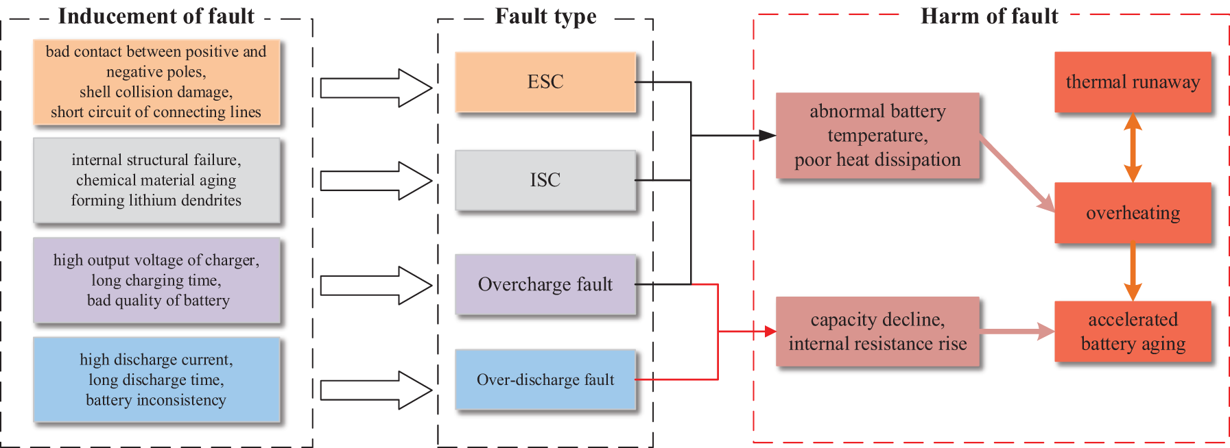
Figure 1: Causes of different faults in the battery system and their coupling relationship

2.2 State Data Analysis

For experimental studies with data-driven models, data analysis is important. Tagade et al. [26] argued that the state data generated by the battery system obeys a normal distribution thus developing the study using a Gaussian process algorithm. This is very advantageous for detection algorithms based on the assumption of normal distribution, which helps the detection results to be more accurate. However, lithium-ion batteries are subject to complex and harsh operating conditions, where disturbances such as external impacts and uneven heat dissipation can cause the battery voltage and temperature data to deviate from a normal distribution, so we also need to perform simple data analysis to explore the relationship between voltage and temperature data when operating EVs under real conditions, as a way to determine the appropriate fault detection algorithm.

This analysis was collected to analyze the normality of the voltage and temperature data generated from the normal operation of the EVs over one month. The normality of the joint distribution of voltage and temperature bivariate is observed as shown in Fig. 2a. From the figure, it can be seen that most of the data are distributed in the voltage range of 3.6~3.8 v, and the temperature is concentrated more in the range of 50°C~55°C, and as shown in Figs. 2b and 2calone from the one-dimensional histogram of voltage and temperature that most of the distribution of the actual data does not conform to the normal distribution. Specifically, the skewness of the voltage data distribution can be seen on the histogram that deviates from the standard value of normal distribution, while the temperature data is more obvious, the skewness and kurtosis deviate from the standard value of normal distribution. This indicates that the distribution pattern of the data has obvious skewness and spikes, rather than the typical bell curve of normal distribution.

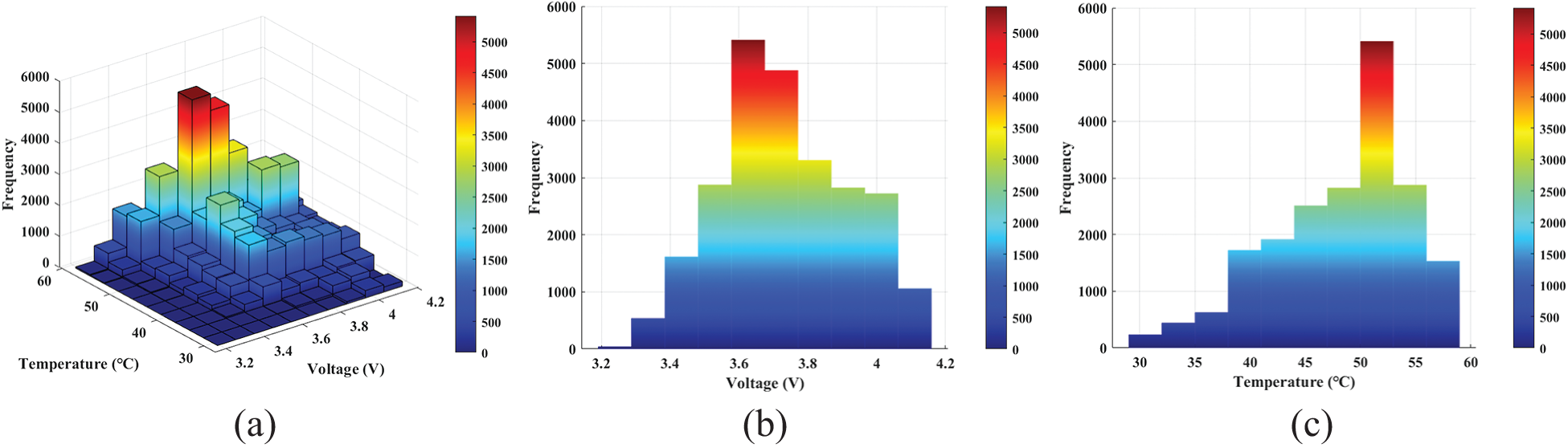
Figure 2: Statistical histogram of battery system status data. (a) Three-dimensional probability density plot, (b) Histogram of voltage data, (c) Histogram of temperature data

It is subjective to determine whether the data conforms to the normal distribution by observing the histogram, in order to ensure the persuasive nature of the data distribution, this paper also considers the use of the Kolmogorov-Smirnov (K-S) test for further clarification. Moreover, this method is generally applicable to the normality test for large sample sizes and is most suitable for the statistical test method of this experiment. Through the null hypothesis that the voltage and temperature data distribution is normal distribution, the test of the truth of the null hypothesis through a single sample of K-S test, comparing the measured distribution and the hypothetical distribution, and the analysis of the data yields the p-value of both to be less than the critical value of α=0.05. Therefore, the null hypothesis is rejected. So, there is a significant difference between the distribution of the data samples and the assumed normal distribution, which is a sufficient indication that the battery system data does not meet the normal distribution.

Therefore, it can be seen that the state data distribution generated by the battery system under actual operating conditions is more complex and does not strictly conform to the Gaussian distribution, and if it is forced to be regarded as a Gaussian distribution for experiments, it is likely to lead to inaccurate and unconvincing experimental results, which will reduce the accuracy and authority of fault detection. Therefore, this paper uses the SVDD algorithm to build a model where the data does not have to conform to the Gaussian distribution.

3  Theory

3.1 Support Vector Data Description

SVDD is an important data description method that enables the distinction between target and non-target samples [21,22]. It is commonly applied in areas such as anomaly detection and fault diagnosis. We represent the train set consisting of the acquired voltage and temperature data by the column vector X=[x1,x2,⋯,xn]T, X∈Rn×d, where n is the number of samples and d is the feature dimension, so we want to obtain a minimal hypersphere description with radius R and center a to include all the training objects xi as much as possible. The objective function is given by Eq. (1):

F(R,a,ξi)=R2+C∑iξi(1)

s.t.(xi−a)T(xi−a)≤R2+ξi   ∀i,ξi≥0

C∑iξi in Eq. (1) is in order to allow for the possibility of outliers in the multidimensional feature space where the distance from the individual sample xi to the center of the sphere a exceeds that of R. The role of the penalty factor C is to take the optimal solution among the hypersphere volume and the sample error. The slack variable ξi is used to weigh the effect of unlabeled partial sample outliers, allowing some of the normal samples to fall outside the hypersphere.

The equation is a convex quadratic programming problem and the undetermined R has not yet been solved. Transform the constrained optimization problem into an unconstrained optimization problem by transforming Eq. (1) into an equivalent Lagrangian dyadic problem and introducing Lagrange multipliers αi and βi to solve the objective function subject to the constraints of the above equation. Construct Primal Lagrange Problem (Minimization):

L(R,a,ξi,αi,βi)=R2+C∑iξi−∑iαi{R2+ξi−(xi−a)T(xi−a)}−∑iβiξi(2)

where the Lagrange multipliers αi≥0, βi≥0. L respond to R, a and ξi minimizing and maximizing for αi and βi. The optimization problem is solved according to the KKT condition. For convex programming problems, the solution satisfying the KKT condition is the global optimal solution. Setting the partial derivative to 0, the solution is obtained as:

∂L∂R:∑iαi=1;∂L∂a:a=∑iαixi∑iαi=∑iαixi;∂L∂ξi:C−αi−βi=0;(3)

Expanding Eq. (2) and substituting the constraints, where we denote the inner product of the target objects xi and xj by (xi⋅xj), gives the dual problem of the original equation as:

L=∑i, jαiαj(xi⋅xj)−∑iαi(xi⋅xi)   (0≤αi≤C,i,j∈N)(4)

Minimizing Eq. (4) yields a set α∗ as the optimal solution:

α∗=(α1,α2⋯αN)(5)

In the data description, when the data sample xi of αi∗>0 is called the support vector (SV), describing its hypersphere also requires only SV. The radius R of the sphere can be obtained from the distance from any SV on the boundary to the center a of the hypersphere. The second equation in Eq. (3) leads to the fact that the center a of the circle of the hypersphere is a linear combination of data samples.

R=1nsv∑s∈sv‖xs−a‖(6)

a=∑iαi∗xi(7)

Due to the constraints and the KKT complementarity condition leading to the inequality constraint, complementary slack βi⋅ξi=0 can determine the location of a sample xi, as shown in Fig. 3.

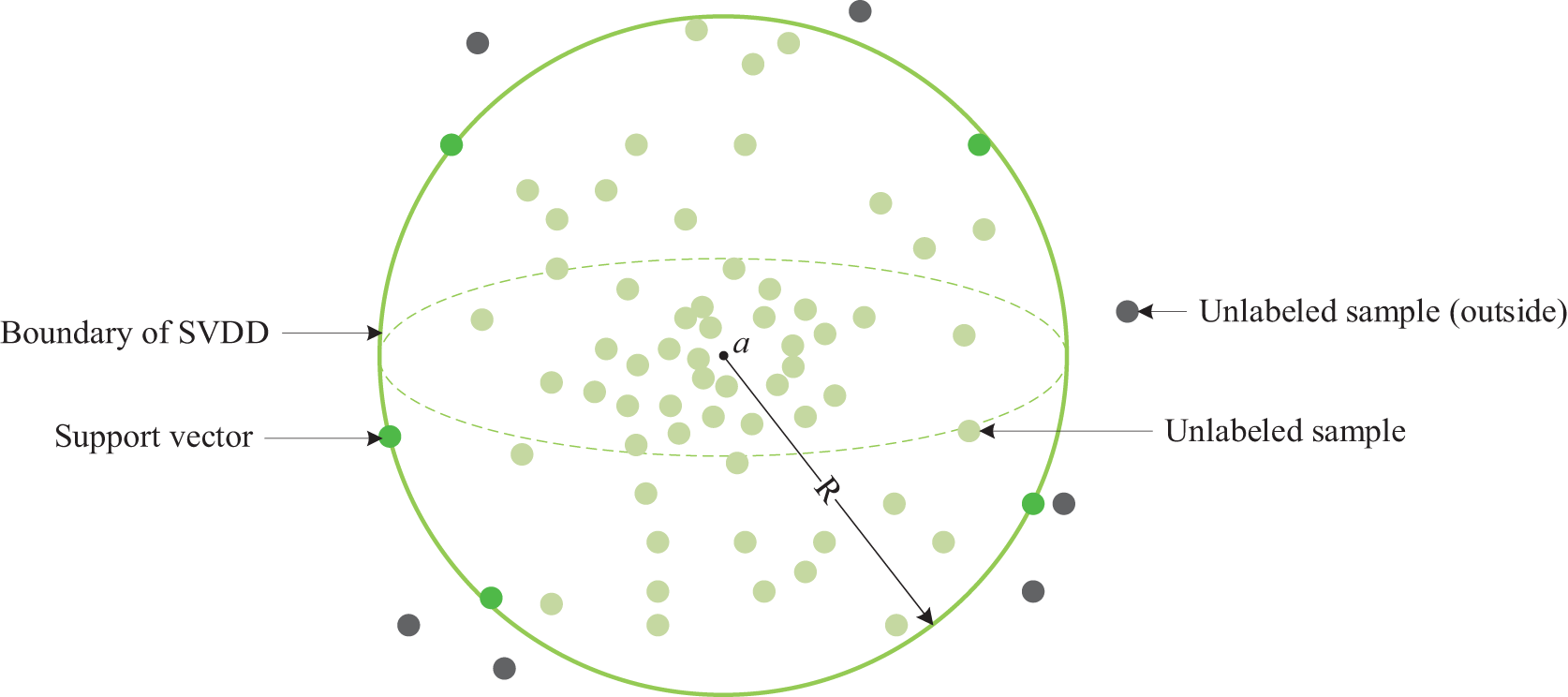
Figure 3: Sketch map of SVDD

Location of a point:

Case 1: αi=0 ⇒ Unlabeled sample

Case 2: 0<αi<C ⇒βi>0 ⇒ξi=0 ⇒ Support vector

Case 3: αi=C ⇒βi=0 ⇒ξi>0 ⇒ Unlabeled sample (outside)

Based on the above detection model, to determine whether the test sample z is located inside the sphere, the distance from the sample to the center of the sphere must be calculated as follows:

RZ2=(z−a)T(z−a)=(z⋅z)−2∑iαi(z⋅xi)+∑i,jαiαj(xi⋅xj)

RZ=(z⋅z)−2∑iαi(z⋅xi)+∑i,jαiαj(xi⋅xj)(8)

When RZ≤R, the test sample is located in the sphere, it is the normal class; otherwise, it is the faulty class.

3.2 Support Vector Data Description with Negative Examples

We can introduce a small number of negative samples into the train set, utilizing the information from these negative samples to refine the hypersphere boundary [22]. This refinement aims to enhance the model’s detection accuracy and prevent overfitting occurrences. When the negative samples within the train set lie within the original SVDD boundary range, minimal adjustments are required for the original boundary, with the negative samples acting as negative support vectors positioned on the NSVDD boundary. In practical engineering applications, the selection of negative samples should be accurate, diverse, and representative. To ensure the accuracy of the selected negative samples, it is essential to avoid choosing similar instances. Encompassing various fault scenarios as comprehensively as possible and adequately reflecting negative samples that depict the operational status can contribute to improving the model’s generalization capabilities.

It is assumed that the subscripts of the detected normal samples are enumerated by i and l, and the subscripts of the faulty samples are enumerated by m and n. The normal samples and faulty samples are labeled as yi=+1 and yj=−1, respectively. Similar to SVDD, both the normal and fault train sets are allowed to have errors, so penalty factors C1 and C2 for both classes of samples and slack variables ξi and ξm are introduced. The objective function is as follows:

F(RN,a,ξi,ξm)=RN2+C1∑iξi+C2∑mξm(9)

s.t.‖xi−a‖2≤RN2+ξi,‖xm−a‖2≥RN2+ξm,ξi≥0,ξm≤0

Introducing Lagrange multipliers αi, αl, βm and βn in Eq. (9), take the partial derivatives of L for RN, a, ξi and ξm:

∑iαi−∑mαm=1

a=∑iαixi−∑mαmxm(10)

C1−αi−βi=0,C2−αm−βm=0,∀i,m

Bringing the above constraints back into the original equation:

L=∑iαi(xi⋅xi)−∑mαm(xm⋅xm)−∑i, lαiαl(xi⋅xl)−∑m, nαmαn(xm⋅xn)+2∑m, lαmαl(xm⋅xl)(11)

Now we define a new variable αi′=yiαi, where the subscript i denotes both the normal sample subscript and the faulty sample subscript so that the constraint in Eq. (10) is changed:

∑iαi−∑mαm=1⇒∑iαi′=1

a=∑iαixi−∑mαmxm⇒a=∑iαi′xi(12)

Bringing the new constraints back into Eq. (11) so that the dual of the original optimization problem becomes:

min∑i, jαi′αj′(xi⋅xj)−∑iαi′(xi⋅xi);(i, j∈N)(13)

According to the dual rule, it can be deduced that the solution form of the NSVDD algorithm and standard SVDD algorithm is the same, and it is only necessary to replace αi with αi′. Therefore, when using NSVDD test samples, it is only necessary to give Lagrange multipliers a category label to get the same solution form and result as ordinary SVDD. That is:

RZ=(z⋅z)−2∑iyiαi(z⋅xi)+∑i, jyiyjαiαj(xi⋅xj)(14)

When RZ≤RN, the test sample is located within the NSVDD sphere which implies it is a normal sample; otherwise, it is a faulty sample.

The ideal NSVDD schematic is shown in Fig. 4, where the model is trained with a large number of unlabeled samples and a small number of faulty samples, where most of the unlabeled samples are normal samples. When the SVDD model is trained using a large number of unlabeled samples, a few faulty samples added will make further adjustments to the boundary of SVDD (dotted green line). A change in the hypersphere boundary means that the original SVs may change. The hypersphere makes a minimum adjustment with the distribution of the new faulty samples, which may make some of the SVs not to be the SVs of the new boundary, and instead of it, the faulty samples closest to the boundary of the sphere make the negative SVs. Thus, the boundary of NSVDD (solid red line) obtains a more accurate hypersphere boundary than the boundary of SVDD and will more accurately detect faults misjudged by SVDD. It should be especially noted that the specific SV variation is based on the data distribution and the results of model training.

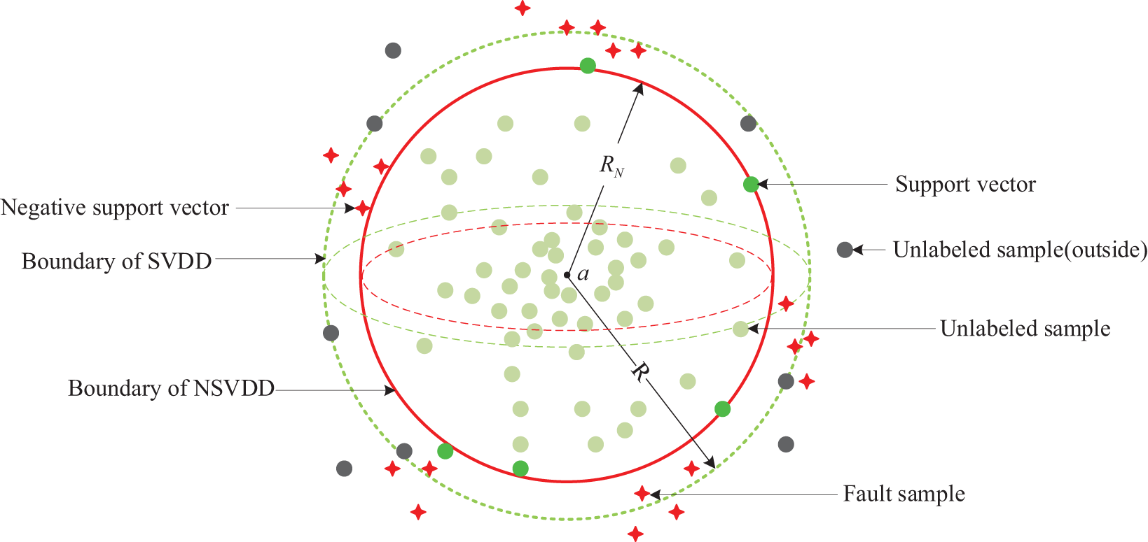
Figure 4: Sketch map of NSVDD

3.3 Kernel Function and Bayesian Optimization

An ideal kernel function maps the target data to a sufficiently high-dimensional feature space to improve the expressive ability of the model. We choose the Gaussian kernel function K(xi,xj) to transform the data to higher dimensions to make the nonlinear data differentiable. The Gaussian kernel function has only one own parameter to be optimized and will produce tighter boundaries, which helps to improve the accuracy of fault detection [27].

K(xi, xj)=exp⁡(−‖xi−xj‖2s2)(15)

Therefore, in this experiment, the detection of the test data z is shown in Eq. (16):

Rz=K(z, z)−2∑iyiαiK(z, xi)+∑i, jyiyjαiαjK(xi, xj)(16)

In machine learning, adjusting parameters is a tedious but crucial task, as it largely affects the performance of the algorithm. Manual tuning of parameters is very time-consuming, and lattices and random searches are not labor-intensive but require long running times. Therefore, many methods for automatic hyperparameter tuning have been born, such as Genetic Algorithms (GA), Particle Swarm Optimization (PSO), Bayesian Optimization, etc. [28]. Through comparative screening, we optimize the hyperparameters by using Bayesian Optimization in this paper, which estimates the posterior distribution of the objective function based on the data using Bayes’ theorem, and then selects the combination of hyperparameters for the next sampling based on the distribution. It makes full use of the information from the previous sampling point, and its optimization works by learning the shape of the objective function and finding the parameters that maximize the result toward the global. It can obtain approximate solutions of complex objective functions with a smaller number of evaluations.

When BO is performed on the hyperparameters of the NSVDD model, we need to define the objective function for optimization. Denoting the hyperparameters in the model as x=(s,C1,C2), where s denotes the Gaussian kernel width parameter, a suitable s significantly improves the classification performance. When s is small, the Gaussian kernel function tends to zero and the optimal solution is obtained only when all objects become SV for αi=1N. When s is large, the solution approximates the original spherical solution. In the normal range, an increase in the parameter s tightens the degree of sphericity described.

We set a total of n sets of hyperparameter combinations xn=(sn,C1,n,C2,n), assuming that a set of hyperparameter combinations is X=(x1,x2,⋯,xn), and the objective function value of each hyperparameter is F(x), which is the loss function we need to optimize. So hyperparameter optimization problem is defined as:

arg⁡minx∈X F(x)(17)

To achieve this goal, we need two main steps to accomplish it: The probability surrogate model and the acquisition function [29].

The objective function and parameter space have been defined, and the optimization process of the objective function is defined next. The tool for estimating the distribution of a function based on a predetermined limited number of observations is the probability surrogate model. In this paper, we use the Gaussian process (GP) as a function of the probability surrogate model used to fit the hyperparameter and output relationship [30]. First, we make assumptions about the initial observation point model to obtain the prior probability distribution P(F), multiply it with the likelihood estimation distribution P(X|F) and normalize it, in which case the resulting proxy model is the posterior probability distribution P(F|X). After the assumed model is computed, it is necessary to maximize the acquisition function based on the probability surrogate model to select the next evaluation point that satisfies the optimization.

The acquisition function is used to measure the impact that the observation points have on the fitted function and to select the most suitable points to perform the next observation [31]. The acquisition function is constructed based on the posterior distribution and the Probability of Improvement is chosen as the acquisition function for the optimization process in this paper. The obtained hyper-parameters are substituted into the function values calculated after training in the network and continue to update the data to re-iterate. This process continues until the combination of parameters that maximizes the generalization ability of the model is filtered out or the computational resources of the setup are fully used up.

4  Data Pre-Processing and Fault Detection Model Framework

4.1 Data Acquisition and Pre-Processing

The data collected in this experiment is obtained from the EVs under normal driving conditions. The battery system of the EVs consists of ternary lithium-ion batteries with a battery voltage range of 2.75~4.5 V and a temperature range of −20°C~60°C. The BMS voltage and temperature acquisition module on the EVs collects a total of 92 dimensions of voltage data and 20 dimensions of temperature data to form the columns of a data state matrix. Therefore, the matrix has 112 columns. Each row of the matrix consists of data values collected by the BMS, with a data recording time interval of 30 s between rows. The computer records such data state matrices and stores them for analysis.

However, due to the measurement error or aging damage of the sensor itself, the complexity of the vehicle driving environment, or interference, there may be relatively uncommon outliers and error values in the collected data, which may affect the battery modeling process, resulting in poor model stability under dynamic conditions. The direct magnitude difference between voltage and temperature is so large that without processing the data, the model will be given more weight in detecting temperature data and be insensitive to voltage data. Data preprocessing is necessary for accurate and reliable data and analytical processing to improve the effectiveness of data analysis and modeling.

This experiment first removes outliers through the 3σ algorithm and the rate of change of each data. Then the data Z-score is standardized and transformed into a uniform scale to improve the comparability of the data, which facilitates the comparison and analysis of the experiment.

After data collection and pre-processing, Table 1 summarizes the train, validation, and test sets used in this experiment, including the labels the total number of samples, and the types and number of faulty samples. Fig. 5 shows the dimensionality reduction and visualization of the dataset. We use t-distributed stochastic neighbor embedding (t-SNE) to reduce the high-dimensional features of the data into a two-dimensional scatter plot showing the distribution and characteristics of normal and faulty samples in these datasets. Where cyan points represent normal samples and orange points represent faulty samples. It can be clearly seen that in the two-dimensional plots of the four fault datasets, the distribution of normal data is relatively uniform and concentrated in the same area. While the fault data distribution is more complex, msf presents a curved form with relatively wide coverage. The occurrence of csf is an extremely slow process, and only with cumulative changes over a period of time does it show obvious fault characteristics. Therefore, csf has a relatively large span of data compared to normal data and exhibits a wider range of variation. The ocf and odf distributions are close to the linear form, which is quite different from the cluster form of the normal data distribution.

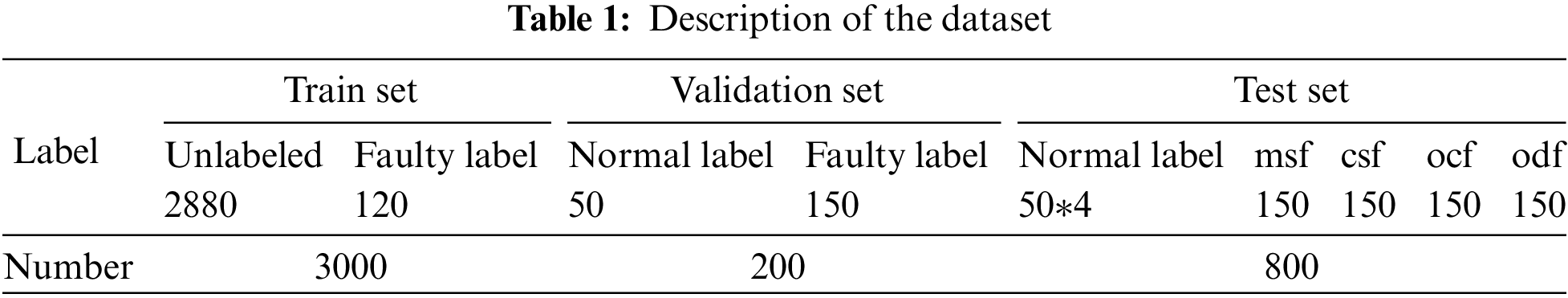
Figure 5: Dimensionality reduction and visualization of datasets. (a) Train set, (b) Validation set, (c) msf set, (d) csf set, (e) ocf set, (f) odf set

Train set: A total of 3000 samples, including 2880 unlabeled samples and 120 faulty samples. The unlabeled samples are mainly normal samples, which are used to train the fault detection model.

Validation set: A total of 50 normal samples with labels and 150 faulty samples with labels to validate the model and adjust the optimization.

Test set: It consists of four fault datasets: msf, csf, ocf, and odf datasets. Each fault dataset consists of 50 normal samples and 150 fault samples from labeling the fault feedback of EVs. The test set has a total of 800 samples and is used to evaluate the trained model.

4.2 Fault Detection Framework

Before conducting the experiments, we need to determine the optimal combination of hyperparameters and create the optimal model for NSVDD fault detection. Combining the theoretical parts of NSVDD and BO in Section 3, as shown in Fig. 6, the training steps of the BO-NSVDD model is as enumerated below:

Figure 6: Fault detection model framework

1. First divide the experimental data into a train set, validation set and test set. In order to build a more accurate detection model, the train set consists of a large amount of unlabeled data, the validation set consists of normal data with labels and faulty data for optimization of the model, and finally, the experiments use the test set to judge the accuracy of the model.

2. Set the Gaussian kernel width s and the positive and negative penalty factors C1 and C2 as the hyperparameter combinations to be optimized, and set the parameter search range and the number of iterations.

3. Use the combination of hyperparameters to be optimized as input to the NSVDD model trained with the train set. The detection error rate of the validation set is taken as the objective function to obtain the minimum value of the objective function.

4. When the minimum value of the objective function is not satisfied, the model is trained by BO iterations until the optimal parameter combination corresponding to the minimized objective function is found or the number of iterations is exhausted. The optimal parameter combination obtained will be tested experimentally in the NSVDD model.

4.3 Practical Application of the Proposed BO-NSVDD Method

The proposed approach is data-driven, which means that it requires only data to train the fault detection model, does not involve the basic working principle of the battery system, and does not require a physical model. As long as the train data is available, the train data can be continuously learned and feature information can be mined from it to achieve accurate fault detection. The practical application of the proposed fault detection model in a battery system is shown in Fig. 7.

Figure 7: Online fault diagnosis framework

1.   Data acquisition and pre-processing

There are more cases of data collected from the battery system that also require manual labeling of small amounts of data, which is combined with a large amount of unlabeled data for training. Obvious and hidden outlier data are eliminated in the preprocessing stage and normalized.

2.   Construction of fault detection model

During offline model training, a large number of unlabeled samples joined with a small number of faulty samples are used to train the base NSVDD model. A small number of labeled samples are combined with BO iterations to train the BO-NSVDD model to achieve optimal classification.

3.   Online applications for fault detection

The trained BO-NSVDD model can then be used in the online fault detection process and applied to the actual equipment or system. Monitor operational data and detect faults or abnormal conditions in real-time as done in the offline model training process. When a fault or abnormal condition is detected, operations such as alarms or stopping work can be triggered to ensure the safe operation of the system.

5  Experiment

5.1 Establishment of BO-NSVDD Detection Model

Before conducting the experiments, a preprocessing step is required for the acquired data. The data preprocessing steps were performed in Python 3.8.5 and Pandas 1.1.5, and the training and testing of the fault detection model were run in MATLAB 2020b. Using the processed, experimental data containing normal and faulty samples, the model is built according to the fault detection framework in Fig. 6, and the validation set data is used for the BO method for automatic adjustment of parameters. The selection of BO as the parameter optimization algorithm is filtered by experimental comparison. The experiments were conducted by comparing three different optimization algorithms for iterative optimization of the hyperparameter combinations of the model, and the same parameter search range, number of seeds, and number of iterations were selected to ensure the consistency of the parameter settings. The experiments of the three optimization algorithms optimized hyperparameter combinations for the test set were repeated 10 times to take the average accuracy and average running time. As shown in Table 2, BO is slightly ahead of PSO and GA in terms of average accuracy, but far ahead in terms of average running time. However, it should be noted that the applicability of the results may be limited due to the specific parameter settings and dataset used in the experiment. Therefore, while BO shows better performance in this experiment, its performance in other contexts still needs to be evaluated with caution.

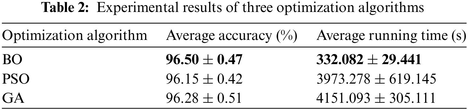
Fig. 8 shows the BO minimum target value vs. the number of iterations when testing the csf fault set. In this experiment, a total of 60 iterations are set, and the BO determines the best feasible point by minimizing the absolute value of the difference between the observed target value and the estimated target value. By empirically setting the search range of hyper-parameter combinations, modeling the model according to its prior distribution, and continuously updating the posterior distribution of model parameters using the existing train data. According to the optimization results, the a priori distribution is updated, and continuously narrowing the parameter search space to find the next feasible point as a way of searching for the optimal parameter combinations. Finally, the observed target value at the 10th iteration is equal to the estimated target value, and the best feasible point observed at this time is the hyperparameter combination with the best final result. Taking this figure to test csf as an example, the final hyperparameter combination (s,C1,C2)=(0.71,0.1121,0.0167) is obtained.

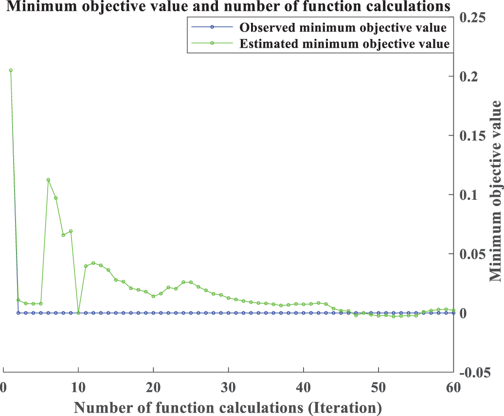
Figure 8: Bayesian optimization of minimum objective value and iteration number process

5.2 Experimental Test Results and Comparisons

Meanwhile, this experiment establishes another five detection models to compare the detection results with the model proposed in this paper, namely BO-SVDD, SVDD, Kernel Principal Components Analysis (KPCA), Principal Components Analysis (PCA), and Deep Autoencoder (DAE). PCA is a linear data dimensionality reduction technique commonly used in industrial system fault detection to determine the presence of abnormal conditions by comparing the principal components of the current data with the normal data state. However, it can generally only handle data with linear relationships and is less practical in data with nonlinear relationships. KPCA is precisely the PCA method for nonlinear data processing, with better data separability and more flexible usage. DAE is a classical unsupervised learning model. In fault detection, DAE recognizes anomalies by reconstructing the input data and observing the reconstruction error. It is also worth noting that the establishmentof the SVDD model does not require the data to obey Gaussian distribution, and the deep structure of the DAE makes it perform better in learning complex data, but the SPE statistics of PCA and KPCA require the data to obey Gaussian distribution. The five comparison models are also implemented in MATLAB 2020b and use the same train and test sets to minimize the accuracy problems caused by data differences. This experiment detects four typical fault categories that are common in real EVs driving: msf, csf, ocf and odf. For each type of fault dataset, the first 50 samples are normal samples. Starting from the 51st sample, the subsequent 150 samples are fault samples. Fig. 9 shows the detection results of six models for various types of faults. In BO-NSVDD, BO-SVDD, and SVDD, the radius of the sphere is used as the boundary for fault detection, which is marked with a red line in the detection plot. Samples within the radius are classified as normal and those beyond the radius are classified as faults. In the experiments with KPCA and PCA, appropriate SPE control limits are set, while for DAE experiments, suitable reconstruction errors are chosen as the respective fault thresholds. Again, the fault thresholds are represented by red lines to distinguish between normal and faulty samples.

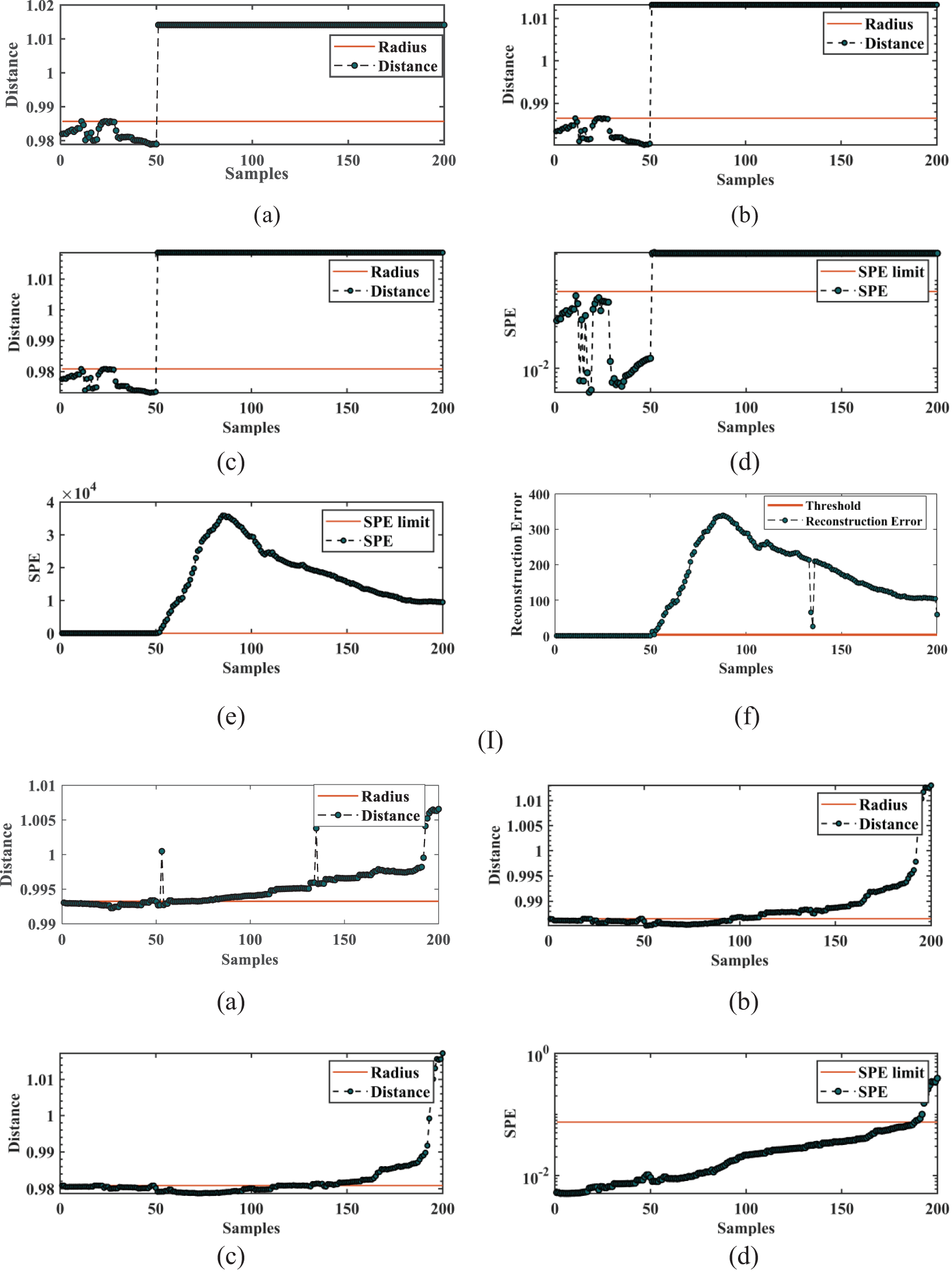
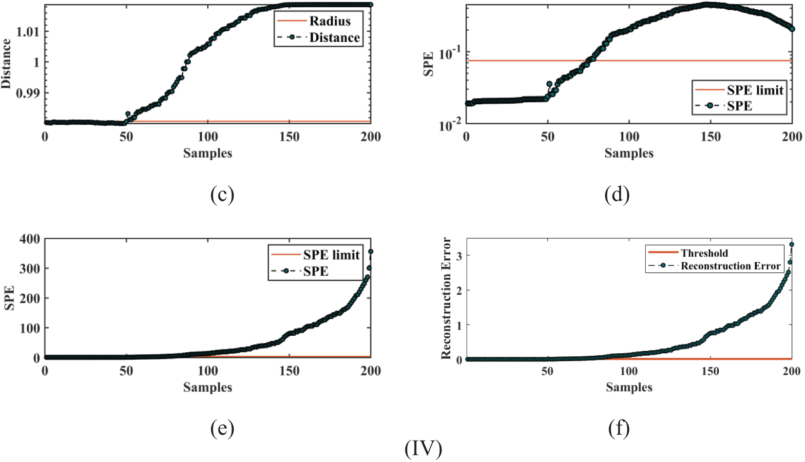
Figure 9: (I) The msf fault detection results of six models: (a) BO-NSVDD detection result, (b) BO-SVDD detection result, (c) SVDD detection result, (d) KPCA detection result, (e) PCA detection result, (f) DAE detection result. (II) The csf fault detection results of six models: (a) BO-NSVDD detection result, (b) BO-SVDD detection result, (c) SVDD detection result, (d) KPCA detection result, (e) PCA detection result, (f) DAE detection result. (III) The ocf fault detection results of six models: (a) BO-NSVDD detection result, (b) BO-SVDD detection result, (c) SVDD detection result, (d) KPCA detection result, (e) PCA detection result, (f) DAE detection result. (IV) The odf fault detection results of six models: (a) BO-NSVDD detection result, (b) BO-SVDD detection result, (c) SVDD detection result, (d) KPCA detection result, (e) PCA detection result, (f) DAE detection result

Fig. 9Ⅰ shows the results of six models for msf detection. The msf is generally an instantaneous short-circuit fault, usually caused by damage to circuit components or external disturbances. This type of fault may lead to a sudden surge in current, resulting in an instantaneous drop in voltage and instability. Components in the circuit are subjected to momentary high current and low voltage, which may cause component damage or burnout, causing a brief high-temperature phenomenon. Therefore, this type of fault occurs when the collected temperature and voltage data vary significantly relative to the normal data. So, each model can accurately detect the occurrence of a fault at the 51st sample, and all have significantly accurate detection for that fault.

However, we know that detecting exceptionally obvious faults does not indicate the superior performance of the model, and the performance of the detection model can only be revealed if some early and minor faults can be detected more quickly and accurately. The csf is exactly the most important fault in this experiment to identify the performance index of the model.

The results of the six models for csf detection are shown in Fig. 9II. Unlike msf, csf refers to the short-circuit phenomenon in a circuit that changes cumulatively over a period of time. The current and voltage in the circuit may change, but the magnitude and speed of the changes are relatively slow, unlike the msf phenomenon which has more pronounced changes. Since the occurrence of cumulative short-circuit faults is a gradual process that is not easily detected in time, this type of fault is the best indicator of the fault detection model. Fig. 9IIa shows the results of csf detection by the BO-NSVDD model. The detection results fluctuate between normal and faulty in the 50th–75th samples, and basically, the occurrence of the fault is detected steadily from the 76th sample, which is faster and earlier than other models. As shown in Fig. 9IIb, BO-SVDD can start to detect the occurrence of faults steadily from the 96th sample, and some of the early and minor faults before that are not detected accurately. Figs. 9IIc and 9IIf show that both SVDD and DAE can start detecting faults at the 111th sample. In contrast, Figs. 9IId and 9IIe show that KPCA and PCA have worse detection capability, detecting faults only when the fault data is sufficiently obvious and having lower detection performance for csf.

Figs. 9III and 9IV show the results of the six models for ocf and odf detection. The detection results of all six models for ocf and odf are relatively good. When overcharge and over-discharge faults occur, the internal chemical reaction of the battery will lead to abnormal changes in battery temperature, voltage, and current, and the longer the duration, the more serious the battery may appear. The three models of BO-NSVDD, BO-SVDD, and SVDD can detect faults earlier and more accurately almost as soon as they occur, with higher fault detection accuracy. The KPCA, PCA, and DAE models, on the other hand, have relatively poor detection results and are more delayed in detecting the moment of fault.

To further illustrate the visual results of the model comparison, this research illustrates the model detection results by plotting the confusion matrix (as shown in Table 3) and using it to create statistical histograms. The confusion matrix is a tool used to evaluate the performance of classification models by comparing the predicted results of the models with the real results to calculate various classification metrics. In this paper, accuracy (ACC) and Area under Curve (AUC) are used to judge and compare the accuracy and classification performance of the six classification models [32].

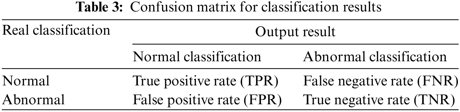
Where, ACC is the accuracy of the classification model, i.e., the ratio of the number of correctly classified samples to the total number of samples. AUC is the area under the Receiver Operating Characteristic Curve (ROC) trapezoidal curve plotted with FPR as the horizontal axis and TPR as the vertical axis, which is used to measure the performance of the classification model. The larger the value of AUC, the better the performance of the classification model, and the better the balance point between the TPR and FPR of the model. The importance of selecting ACC and AUC as model performance metrics in this experiment is that their combined use can help us evaluate the classification performance of the model for different classes of samples. ACC can measure the classification effectiveness of the model for the overall sample, unlike ACC. AUC, on the other hand, measures the model’s ability to distinguish between positive and negative samples, which can avoid the effect of sample imbalance. Therefore, in the case of sample imbalance, AUC can better reflect the classification effect of the model. Therefore, the combination of the two can provide a more comprehensive assessment of the classification performance of the model and thus better guide the optimization and selection of the model. ACC and AUC calculation formulas are shown in Eqs. (18) and (19), respectively, where P is the number of positive samples, N is the number of negative samples and ranki denotes the ordinal number that ranks the probability of predicting a positive sample from smallest to largest.

ACC=TP+TNTP+TN+FP+FN(18)

AUC=∑i∈positiveClassranki−P(1+P)2P×N(19)

As shown in Fig. 10, this histogram puts together the ACC and AUC of the six classification models for the four fault datasets, which gives a more intuitive view of the detection effectiveness of each model for the same fault. For csf, the PCA and KPCA models have almost the same detection effect while SVDD, although more accurate than these two models, is inferior to DAE and BO-SVDD. BO-NSVDD, on the other hand, is in the absolute leading position in terms of accuracy in processing csf. For msf, ocf and odf, BO-NSVDD has also been having an excellent detection effect.

Figure 10: ACC and AUC performance indicators of PCA, KPCA, DAE, SVDD, BO-SVDD and BO-NSVDD on four fault data sets. (a) ACC result, (b) AUC result

In addition, as shown in the AUC detection histogram, the AUC values for all models are at a high level for all three fault detection except csf detection, and even several models have an AUC value of 1 for the fault data set, although their corresponding ACC do not reach 100%. This is because the model does a better job of distinguishing between positive and negative samples in the case of sample imbalance. AUC is evaluated probabilistically based on the distance between positive and negative samples at different thresholds, which only considers the ranking relationship between positive and negative samples, while ACC is based on the exact fault threshold, and improper thresholding will lead to a decrease in ACC. For the detection results of csf, the AUC values of PCA and KPCA are higher than those of SVDD, DAE and BO-SVDD, but the AUC values of BO-NSVDD are also in a clear lead. Overall, the ACC and AUC values of the BO-NSVDD model are at a very high level and significantly better than the other five models for all four fault datasets.

5.3 Robustness Experiments

During the actual operation of EVs, which is often accompanied by the disturbing influence of various harsh conditions, the state data collected by the BMS is easily disturbed, and some residual and abnormal values are eliminated when the data pre-processing step is carried out. In addition, measurement errors caused by noise interference such as battery system vibration collision, weak noise, and strong magnetic environment are also unavoidable in normal driving. In order to verify the effectiveness and accuracy of the proposed method, this research also needs to conduct robustness experimental tests on the proposed model. According to QC/T 897-2011 and GB/T 38661-2020 in the “Technical Conditions for Battery Management Systems for Electric Vehicles”, the voltage measurement error of the lithium-ion battery pack should not be higher than 0.5% of the full range. Therefore, we integrated the four fault-type datasets performed in the experiments into one dataset and added 60–80 dB of Gaussian white noise from strong to weak to measure the robustness of the models under different noise level disturbances. The results are shown in Fig. 11 for the experimental comparison of the robustness of the ACC and AUC performance metrics for the PCA, KPCA, DAE, SVDD, BO-SVDD, and BO-NSVDD models.

Figure 11: Experimental comparison of the robustness of ACC and AUC performance indicators for PCA, KPCA, DAE, SVDD, BO-SVDD and BO-NSVDD. (a) ACC result, (b) AUC result

In noisy datasets, the boundary between normal and faulty samples may be more blurred due to the presence of noise interference, making it more difficult to distinguish them. In the 60~80 dB signal-to-noise ratio interval in this experiment, the accuracy of DAE, SVDD, BO-SVDD, and BO-NSVDD models is significantly ahead of PCA and KPCA. Among them, in 60~72 dB, the difference in detection accuracy of DAE, SVDD, BO-SVDD, and BO-NSVDD models is very slight, but in 72~80 dB noise, the accuracy of the BO-NSVDD model increases and leads the other models. It shows that the model is more resistant to noisy data and can classify more accurately and maintain a higher accuracy.

In addition, as shown in Fig. 11b, the AUC values of the six models under the influence of noise are compared, except for the AUC value of the PCA model, which is less stable and varies widely, indicating that PCA is more susceptible to noise and interference in the data and less robust. The AUC values of the other five models have been in a stable amplitude range, and the stable AUC values indicate that the performance of the model is consistent across different data sets, i.e., the model has a more stable prediction ability for different samples. This indicates that the model has a good generalization ability and can cope with unseen data better. Therefore, all five models except PCA are robust to noise and disturbances in the data and are not easily affected by outliers or noisy data. Especially in comparison, the BO-NSVDD model has the highest AUC value under different noise levels, and the accuracy and robustness of the BO-NSVDD model proposed in this experiment have a good precision in the overall comparison, which is of strong significance for practical applications.

6  Conclusion

In this paper, a data-driven method based on semi-supervised learning combined with the NSVDD method is proposed for the problem of fault detection in the safe and reliable operation of lithium-ion battery EVs, which can accurately and quickly detect the early and minor faults in the fault detection of the battery system. The method firstly preprocesses the collected voltage and temperature data, and then nonlinearly maps a large number of unlabeled samples and a small number of faulty samples into a high-dimensional space. In order to solve the problem of missed detection caused by the unbalanced distribution of abnormal samples, the faulty samples are incorporated into the basic SVDD model training, which aims at better modifying the hypersphere boundary, avoiding the missed detection of faulty samples and preventing the occurrence of overfitting phenomenon. Then a small amount of labeled data is fully utilized for BO, which greatly improves the efficiency of finding the optimal parameters. In the experiments, four datasets of common fault types of EVs are used for validation and comparison with other five fault detection models, and the experimental results show that the detection performance of the method proposed in this paper maintains a high level in the four types of fault data, especially in the early and imperceptible minor faults, and the detection accuracy also has a significant advantage. In addition, robustness experiments are also conducted on six models, and the ACC and AUC values are evaluated as model performance indicators, and the experimental results verify that the method proposed in this paper has strong robustness and generalizability.

In future work, there is a need to explore in depth how to extend the NSVDD theorem to some other improved SVDD methods. The fault isolation function of the SVDD model also needs to be further developed so that the method can accurately and quickly locate the fault that occurs when it has outstanding detection performance, not only to improve the safety of EVs driving but also to facilitate the subsequent maintenance work.

Acknowledgement: The authors acknowledge the reviewers and editors for providing valuable comments and helpful suggestions to enhance the manuscript.

Funding Statement: This work is supported partially by National Natural Science Foundation of China (NSFC) (No. U21A20146), Collaborative Innovation Project of Anhui Universities (No. GXXT-2020-070), Cooperation Project of Anhui Future Technology Research Institute and Enterprise (No. 2023qyhz32), Development of a New Dynamic Life Prediction Technology for Energy Storage Batteries (No. KH10003598), Opening Project of Key Laboratory of Electric Drive and Control of Anhui Province (No. DQKJ202304), Anhui Provincial Department of Education New Era Education Quality Project (No. 2023dshwyx019), Special Fund for Collaborative Innovation between Anhui Polytechnic University and Jiujiang District (No. 2022cyxtb10), Key Research and Development Program of Wuhu City (No. 2022yf42), Open Research Fund of Anhui Key Laboratory of Detection Technology and Energy Saving Devices (No. JCKJ2021B06), Anhui Provincial Graduate Student Innovation and Entrepreneurship Practice Project (No. 2022cxcysj123) and Key Scientific Research Project for Anhui Universities (No. 2022AH050981).

Author Contributions: The authors confirm contribution to the paper as follows: Formal analysis, Writing-original draft preparation, Visualization: Miao Li; Methodology, Conceptualization, Validation, Supervision: Fanyong Cheng; Data acquisition, Writing-reviewing and Editing: Jiong Yang; Writing-reviewing and Editing: Maxwell Mensah Duodu, Hao Tu. All authors reviewed the results and approved the final version of the manuscript.

Availability of Data and Materials: Due to the nature of this research, participants of this study did not agree for their data to be shared publicly, so supporting data is not available.

Conflicts of Interest: The authors declare that they have no conflicts of interest to report regarding the present study.

References

1. Y. Zhao, P. Liu, Z. Wang, L. Zhang, and J. C. Hong, “Fault and defect diagnosis of battery for electric vehicles based on big data analysis methods,” Appl. Energy, vol. 207, pp. 354–362, Dec. 2017. doi: 10.1016/j.apenergy.2017.05.139. [Google Scholar] [CrossRef]

2. S. B. Sarmah et al., “A review of state of health estimation of energy storage systems: Challenges and possible solutions for futuristic applications of Li-ion battery packs in electric vehicles,” ASME J. Electrochem. En. Conv. Stor., vol. 16, no. 4, pp. 40801, Nov. 2019. doi: 10.1115/1.4042987. [Google Scholar] [CrossRef]

3. O. Aiello, “Electromagnetic susceptibility of battery management systems’ ICs for electric vehicles: Experimental study,” Electronics, vol. 9, no. 3, pp. 510, Mar. 2020. doi: 10.3390/electronics9030510. [Google Scholar] [CrossRef]

4. O. Aiello, P. S. Crovetti, and F. Fiori, “Susceptibility to EMI of a battery management system IC for electric vehicles,” in 2015 IEEE Int. Symp. Electromagn. Compat. (EMC), Dresden, Germany, 2015, pp. 749–754. [Google Scholar]

5. M. K. Tran and M. Fowler, “A review of lithium-ion battery fault diagnostic algorithms: Current progress and future challenges,” Algorithms, vol. 13, no. 3, pp. 62, Mar. 2020. doi: 10.3390/a13030062. [Google Scholar] [CrossRef]

6. L. Lu, X. Han, J. Li, J. Hua, and M. Ouyang, “A review on the key issues for lithium-ion battery management in electric vehicles,” J. Power Sources, vol. 226, pp. 272–288, Mar. 2013. doi: 10.1016/j.jpowsour.2012.10.060. [Google Scholar] [CrossRef]

7. X. Hu, K. Zhang, K. Liu, X. Lin, S. Dey and S. Onori, “Advanced fault diagnosis for lithium-ion battery systems: A review of fault mechanisms, fault features, and diagnosis procedures,” IEEE Ind. Electron. Mag., vol. 14, no. 3, pp. 65–91, Sep. 2020. doi: 10.1109/MIE.2020.2964814. [Google Scholar] [CrossRef]

8. C. Wu, C. Zhu, Y. Ge, and Y. Zhao, “A review on fault mechanism and diagnosis approach for Li-ion batteries,” J. Nanomat., vol. 631263, pp. 8, 2015. doi: 10.1155/2015/631263. [Google Scholar] [CrossRef]

9. Z. Gao, C. Cecati, and S. X. Ding, “A survey of fault diagnosis and fault-tolerant techniques—Part I: Fault diagnosis with model-based and signal-based approaches,” IEEE Trans. Ind. Electron., vol. 62, no. 6, pp. 3757–3767, Jun. 2015. doi: 10.1109/TIE.2015.2417501. [Google Scholar] [CrossRef]

10. G. Zhiwei, C. Cecati, and S. X. Ding, “A survey of fault diagnosis and fault-tolerant techniques—Part II: Fault diagnosis with knowledge-based and hybrid/active approaches,” IEEE Trans. Ind. Electron., vol. 62, no. 6, pp. 3768–3774, Jun. 2015. doi: 10.1109/TIE.2015.2419013. [Google Scholar] [CrossRef]

11. J. Yu and Y. Zhang, “Challenges and opportunities of deep learning-based process fault detection and diagnosis: A review,” Neural Comput. Appl., vol. 35, no. 1, pp. 211–252, Jan. 2023. doi: 10.1007/s00521-022-08017-3. [Google Scholar] [CrossRef]

12. J. Yang, F. Y. Cheng, Z. Liu, M. M. Duodu, and M. Zhang, “A novel semi-supervised fault detection and isolation method for battery system of electric vehicles,” Appl. Energy, vol. 349, pp. 121650, Nov. 2023. doi: 10.1016/j.apenergy.2023.121650. [Google Scholar] [CrossRef]

13. Z. J. Zhang et al., “Battery leakage fault diagnosis based on multi-modality multi-classifier fusion decision algorithm,” J. Energy Storage, vol. 72, pp. 108741, Nov. 2023. doi: 10.1016/j.est.2023.108741. [Google Scholar] [CrossRef]

14. J. E. van Engelen and H. H. Hoos, “A survey on semi-supervised learning,” Mach. Learn., vol. 109, pp. 373–440, Feb. 2020. doi: 10.1007/s10994-019-05855-6. [Google Scholar] [CrossRef]

15. S. R. Hashemi, A. B. Baghbadorani, R. Esmaeeli, A. Mahajan, and S. Farhad, “Machine learning-based model for lithium-ion batteries in BMS of electric/hybrid electric aircraft,” Int. J. Energy Res, vol. 45, no. 4, pp. 5747–5765, Mar. 2021. doi: 10.1002/er.6197. [Google Scholar] [CrossRef]

16. O. Ojo, H. Lang, Y. Kim, X. Hu, B. Mu and X. Lin, “A neural network based method for thermal fault detection in lithium-ion batteries,” IEEE Trans. Ind. Electron., vol. 68, no. 5, pp. 4068–4078, May 2021. doi: 10.1109/TIE.2020.2984980. [Google Scholar] [CrossRef]

17. K. Das, R. Kumar, and A. Krishna, “Analyzing electric vehicle battery health performance using supervised machine learning,” Renew. Sustain. Energ. Rev., vol. 189, pp. 113967, Jan. 2024. doi: 10.1016/j.rser.2023.113967. [Google Scholar] [CrossRef]

18. Q. Xue, G. Li, Y. J. Zhang, S. Q. Shen, Z. Chen and Y. G. Liu, “Fault diagnosis and abnormality detection of lithium-ion battery packs based on statistical distribution,” J. Power Sources, vol. 482, pp. 228964, Jan. 2021. doi: 10.1016/j.jpowsour.2020.228964. [Google Scholar] [CrossRef]

19. F. Zhang, Z. X. Xing, and M. H. Wu, “Fault diagnosis method for lithium-ion batteries in electric vehicles using generalized dimensionless indicator and local outlier factor,” J. Energy Storage, vol. 52, pp. 104963, Aug. 2022. doi: 10.1016/j.est.2022.104963. [Google Scholar] [CrossRef]

20. W. Guo, L. Yang, Z. Deng, B. Xiao, and X. Bian, “Early diagnosis of battery faults through an unsupervised health scoring method for real-world applications,” IEEE Trans. Transp. Electr., Aug. 2023. doi: 10.1109/TTE.2023.3300302. [Google Scholar] [CrossRef]

21. D. M. Tax and R. P. Duin, “Support vector domain description,” Pattern Recognit. Lett., vol. 20, no. 11–13, pp. 1191–1199, Nov. 1999. doi: 10.1016/S0167-8655(99)00087-2. [Google Scholar] [CrossRef]

22. D. M. Tax and R. P. Duin, “Support vector data description,” Mach. Learn., vol. 54, pp. 45–66, Jan. 2004. doi: 10.1023/B:MACH.0000008084.60811.49. [Google Scholar] [CrossRef]

23. J. B. Robinson et al., “Microstructural analysis of the effects of thermal runaway on Li-ion and Na-ion battery electrodes,” ASME. J. Electrochem. En. Conv. Stor., vol. 15, no. 1, pp. 11010, Feb. 2018. doi: 10.1115/1.4038518. [Google Scholar] [CrossRef]

24. Q. Hou, J. Liu, J. X. Zhang, Z. H. Xu, X. Chen and P. Chen, “A vehicle alarm network for high-temperature fault diagnosis of electric vehicles,” Appl. Intell., vol. 53, no. 6, pp. 6230–6247, Mar. 2023. doi: 10.1007/s10489-022-03615-z. [Google Scholar] [CrossRef]

25. R. Xiong, W. Z. Sun, Q. Q. Yu, and F. C. Sun, “Research progress, challenges and prospects of fault diagnosis on battery system of electric vehicles,” Appl. Energy, vol. 279, pp. 115855, Dec. 2020. doi: 10.1016/j.apenergy.2020.115855. [Google Scholar] [CrossRef]

26. P. Tagade et al., “Deep Gaussian process regression for lithium-ion battery health prognosis and degradation mode diagnosis,” J. Power Sources, vol. 445, pp. 227281, Jan. 2020. doi: 10.1016/j.jpowsour.2019.227281. [Google Scholar] [CrossRef]

27. Y. T. Xue, L. Zhang, B. J. Wang, Z. Zhang, and F. Z. Li, “Nonlinear feature selection using Gaussian kernel SVM-RFE for fault diagnosis,” Appl. Intell., vol. 48, pp. 3306–3331, Oct. 2018. doi: 10.1007/s10489-018-1140-3. [Google Scholar] [CrossRef]

28. L. Yang and A. Shami, “On hyperparameter optimization of machine learning algorithms: Theory and practice,” Neurocomputing, vol. 415, pp. 295–316, Nov. 2020. doi: 10.1016/j.neucom.2020.07.061. [Google Scholar] [CrossRef]

29. P. I. Frazier, “Bayesian optimization,” in INFORMS TutORials in Operations Research, INFORMS, 2018, pp. 255–278. doi: 10.1287/educ.2018.0188 [Google Scholar] [CrossRef]

30. M. Seeger, “Gaussian processes for machine learning,” Int. J. Neural Syst., vol. 14, no. 2, pp. 69–106, 2004. doi: 10.1142/S0129065704001899. [Google Scholar] [PubMed] [CrossRef]

31. J. Snoek, H. Larochelle, and R. P. Adams, “Practical bayesian optimization of machine learning algorithms,” Advances in neural information processing systems,” in Proc. 25th Int. Conf. Neural Inform. Process. Syst., Dec. 2012, pp. 2951–2959. [Google Scholar]

32. J. Huang and C. X. Ling, “Using AUC and accuracy in evaluating learning algorithms,” IEEE Trans. Knowl. Data Eng., vol. 17, no. 3, pp. 299–310, Mar. 2005. doi: 10.1109/TKDE.2005.50. [Google Scholar] [CrossRef]