Evaluation of Multi-Temporal-Spatial Scale Adjustment Capability and Cluster Optimization Operation Method for Distribution Networks with Distributed Photovoltaics

Nomenclature

1  Introduction

Driven by the objective of achieving carbon neutrality, the global consensus has emerged on the prioritized development of clean energy, particularly in the forms of PV and wind power [1]. As the world’s largest consumer of energy production and the fastest-growing user of energy, China has set ambitious targets to reach carbon peak by 2030 and achieve carbon neutrality by 2060 [2]. It is anticipated that the proportion of PV power generation in the future energy supply will gradually increase, with distributed PV systems enjoying the advantages of local consumption and a small footprint [3]. These systems have been strongly supported by various policies. However, PV power generation exhibits strong uncertainty and randomness, and the dense interconnection of numerous distributed PV systems to the grid leads to increasingly complex system operations within distribution stations [4,5], resulting in occasional instances of light abandonment [6]. Therefore, it is of great significance to evaluate the capacity for adjustment within the distributed PV station area and coordinate the economic and adjustment performance of the station area, aiming to reduce operating costs within distribution stations, improve the local consumption of PV energy, and promote clean energy transformation.

The cluster management mode offers distinct advantages in addressing renewable energy access and on-site consumption. When dealing with a large and geographically diverse number of power supplies, the cluster management mode has garnered increasing attention and application due to its unique characteristics of “weak coupling among groups and cooperation through division of labor and strong connection within groups” [7,8]. Reference [9] carry out cluster division and management by calculating the electrical distance between nodes within the cluster and between clusters. References [10,11] introduced a method for defining and dividing indicators based on electrical distance, utilizing the relationship between node voltages to cluster distributed power supply nodes. References [12,13] emphasize that various factors such as adjustment cost, response characteristics, geographical location, and other characteristics of distributed power supply must be considered during cluster division of distributed power supply. The cluster division method proposed in references [14–16], which is based on planning classes, takes into account the power complementary characteristic relationship between nodes and addresses the issue of source-load matching. While the studies on cluster partitioning index and partitioning algorithm in the aforementioned literature are comprehensive, they fail to consider the assessment of adjustment capacity post-clustering and do not fully account for the adjustment capacity of source network load and storage within the cluster. Consequently, the outcome of cluster partitioning hinders the utilization of resource adjustment capacity, thereby impeding the consumption of renewable energy under the cluster management mode.

The primary challenge in assessing adjustment capacity lies in quantifying the adequacy of adjustment resources and reflecting their availability. To date, domestic and international researchers have achieved some notable findings regarding the evaluation of the regulation capacity of distribution stations that incorporate distributed PVs. Reference [17] references the traditional power shortage expectation index and introduces a metric for assessing the expected index of resource shortage and climbing, as well as adjustment capacity, from the perspective of meeting net load demand. References [18,19] address system operation mode using economic scheduling models, compute flexibility indices from the perspectives of load loss and wind energy abandonment and introduce practical flexibility index evaluation methods. Reference [20] introduces metrics for power supply up-regulation and down-regulation flexibility margins and builds a multi-source coordinated optimization model based on these constraints. Reference [21] considers supply and demand power balance as well as energy balance and introduces flexibility evaluation indexes suitable for transition scenarios in high-proportion new energy power systems. References [22,23] quantify the demand and supply of multi-time scale flexibility based on spectral analysis. Overall, the aforementioned studies primarily focus on the balance between supply and demand, with few considering whether line transmission capacity can meet regulatory demands in terms of regulatory capacity assessment. References [24–27] emphasize the significance of considering line transmission capacity in the study of flexibility. Reference [24] defines the flexibility index for grid frames, but it employs a fixed power output evaluation system for flexibility, which renders the flexibility evaluation impractical. In reference [25], line transmission capacity is treated as a constraint condition, and a probabilistic index is employed to evaluate system flexibility, which is suitable for system planning and decision-making. Reference [26] proposes the concept of flexibility carrying capacity by considering the transmission carrying capacity of lines and performs system expansion planning based on this, but it may result in significant expansion costs. Reference [27] considers the positive role of the complementary energy hub flexibility on both the supply and demand sides in promoting renewable energy consumption, avoiding load losses, and alleviating line congestion. However, none of these studies have been applied to the assessment of regulation capabilities. The aforementioned references evaluated the flexibility of regulatory resources using indicators such as new energy acceptance capacity, elasticity, reliability, and line transmission indicators. However, most studies employed indicators to indirectly reflect the regulatory capacity of regulatory resources without considering the assessment of post-cluster regulatory capacity and the impact of line transmission capacity on the assessment of regulatory capacity. The mapping relationship between the adjustment of regulatory resources and the economy of distribution network operation has not been established.

Addressing the shortcomings of existing literature, this paper introduces a multi-temporal scale adjustment capability assessment technique for distribution networks with distributed PVs, considering various geographical locations, coverage areas, and response capabilities. The key contributions are outlined below:

1) This study analyzes the multi-temporal scale adjustment characteristics and response capabilities of different adjustment resources in distribution networks. Based on their inherent features, a calculation method for adjustment capabilities is proposed, taking into account the adjustment status and boundary constraints of these resources. Furthermore, a model is constructed that balances physical states and user behaviors to assess the maximum adjustable range of various adjustment resources, including electric vehicles, energy storage devices, gas turbines, and controllable loads.

2) Considering line capacity limitations, indices for assessing the adjustment capability boundary and margin of distribution networks are introduced. The adjustment capability margin index, which builds upon the boundary index, comprehensively considers line transmission constraints to evaluate the adjustment capabilities of distribution networks within their transmittable range.

3) Utilizing electrical distance-based modularity indicators and active power balance indicators as comprehensive criteria, a genetic algorithm-based clustering method is proposed. Incorporating both distribution network safety constraints and adjustment resource constraints, an economic optimization model is established to minimize the economic costs of the distribution network. Finally, the effectiveness of the proposed assessment technique in enhancing the adjustment capabilities, reducing economic losses, and improving the consumption capacity of PVs is validated through a modified IEEE33-node case study.

The remainder of this article is organized as follows. In the Section 2, a regulation model for distribution station area adjustment resources is established. The Section 3 introduces the evaluation indicators for the adjustment capacity of the distribution station area. The Section 4 presents a clustering method for the distribution station area, along with an economic optimization model. The Section 5 provides a case study, and the sixth section concludes the article.

2  Analysis of Resource Regulation Characteristics in Distribution Station Area

2.1 Multi-Time Scale Adjustment Capability Analysis of Distribution Station Area Resources

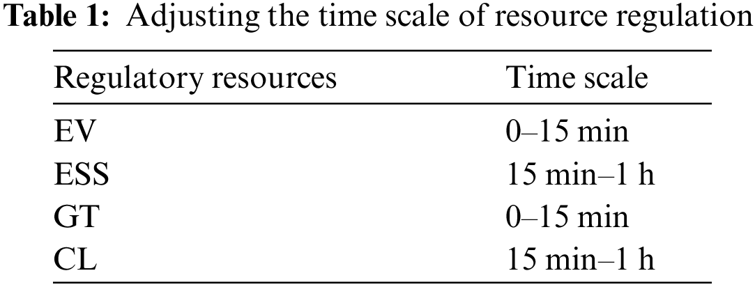
The regulation resources in the distribution station area mainly include electric vehicles (EV), energy storage systems (ESS), diesel units, gas turbines (GT) and controllable load (CL). The regulating capacity of a platform area is related to the operating state of each regulating resource and its output regulating characteristics. The same regulation resource has different regulation characteristics under different time scales, and the regulation characteristics of different regulation resources are also different under the same time scale. This section analyzes the adjustment characteristics of each adjustment resource and establishes the adjustment capacity models of the adjustment resources of the platform area at different time scales. The adjustment time scales of each adjustment resource are shown in Table 1.

2.2 EV Regulating Capacity

2.2.1 Physical Characteristics

The EV features two control modes: G2V and V2G. In situations where the system’s upward regulation capacity is inadequate, the EV can adjust by reducing its charging power via G2V control or discharging power to the grid via V2G control. Conversely, when the system’s downward regulation capacity is insufficient, the EV can compensate by increasing its charging power via G2V control [28]. The dynamic characteristics of EVs are described by changes in battery power, as follows:

S(t)=ηPev(t)/Eev,η={ηc,Charge1/ηd,Discharge(1)

where, S(t) is the state of charge (SOC) of the EV battery; η is the charging and discharging efficiency of EV; Pev(t) is the power of EV at time t; Eev is the rated capacity of the EV battery; ηc, ηd is the charging and discharging efficiency of EV, which is generally a fixed parameter related to the EV model.

To ensure the safety of the battery and charging pile, EV operation must adhere to power and power constraints, as follows:

Sev,min≤S(t)≤Sev,max(2)

−Pev,dmax≤Pev(t)≤Pev,cmax(3)

where, Sev,max, Sev,min are the upper and lower limits of SOC allowed for EV operation, determined by battery characteristics; Pev,cmax, Pev,dmax are the maximum charging and discharging power of the EV, determined jointly by the charging station and the battery. EVs that can discharge into the grid are usually referred to as V2G type, while EVs that cannot discharge in reverse (Pev,dmax = 0) are referred to as V1G type [29].

How the user utilizes the vehicle and its charging parameters dictate the extent to which the EV can provide regulation. EV participation in regulation is limited to the grid-connected period and can be characterized by tin at the on-grid time and tout at the off-grid time, which reflect the vehicle owner’s habits. The EV charging target must be guaranteed, as specified by Smin,exp, the minimum expected state of charge that must be achieved when off-grid. The user can also impose constraints such as whether to allow EV discharge, the number of discharges within a specified cycle, or the maximum discharge depth [30–32].

2.2.2 Assessment of EV Regulation Capacity

Leveraging the physical characteristics and user behavior constraints, the evaluation of EV power regulation capability is translated into an optimization problem for optimal value solutions.

S(t)={S(t0)+∫t0t(Pev(t)+ΔP)η/Eevdttin≤t0<t≤t0+TS(t0+T)+∫t0+TtoutPevcomp(t)η/Eevdtt0+T<t≤tout(4)

Sev,min≤S(t)≤Sev,max(5)

Smin,exp≤S(tout)(6)

−Pev,dmax≤Pev(t)−ΔP≤Pev,cmax(7)

−Pev,dmax≤Pevcomp(t)≤Pev,cmax(8)

where, ΔP is the power change of the EV, the maximum value for positive corresponds to the down regulation ability, and the minimum value for negative corresponds to the up regulation ability; T is used to adjust the time scale; Pevcomp(t) is the EV operating power after the adjustment is completed. Eq. (4) represents the state changes during and after EV power regulation, Eqs. (5) and (6) represent the SOC constraints during EV grid connection and off grid time, and Eqs. (7) and (8) represent the EV charging and discharging power constraints during and after power regulation.

The process of EV state transfer can be described intuitively based on the t-S plane, and the participation in power regulation corresponds to the change of its state trajectory. The adjustment ability is the maximum trajectory that meets the change under constraints, and the EV operating range and constraints are shown in Fig. 1. The adjustment capability is defined as the maximum trajectory shift within given constraints. The feasible region defined by Eqs. (4)–(8) is outlined by curves ①–⑥. Here, ①, ② represents SOC constraints, ③, ④ power constraints, ⑤ off-grid time constraints, and ⑥ is the forced charging curve determined by the expected SOC and maximum charging power off-grid. Over time, curves ③ and ④ shift rightward, narrowing the feasible region. The tracks I, II, III, and IV in the figure correspond to four potential charging and discharging modes: Charging-standing, charging-standing, charging-charging, and discharging-charging-standing. The actual charging mode depends on the chosen charging strategy.

Figure 1: EV operating range and constraints

Trajectory IV is used as a representative example to illustrate the EV power regulation process. Here, trajectory a serves as the baseline trajectory. Trajectory b represents the adjustment process undergone by the EV, where discharge is employed to compensate for power shortages. However, the adjustment capacity is constrained by the minimum power required to meet the user’s charging time requirements. Track c illustrates the adjustment process under EV conditions, where charging is maximized to cope with excess power. Again, the adjustment capacity is limited by the maximum power allowed to meet the user’s charging time requirements. In practice, as EV state changes and other factors such as regulation time T vary, the calculation of EV power regulation capacity may encounter various constraints.

When calculating the upper adjustment capacity, constraints ①, ④, or ⑥ (reverse discharge adjustment) may be activated, or only constraint ⑥ may be triggered (only charge power adjustment). The activation of these constraints depends on the SOC relationship before and after power adjustment. Once the adjustment is complete and constraint ⑥ is activated, the EV is situated on curve ⑥ or its extended dotted line, at which point the state of charge (SOC) is:

So=Smin,exp−ηcPev,cmax(tout−t0−T)/Eev(9)

If SO<S(t0), then constraints ①, ④, and ⑥ may be activated, in which case the maximum discharge power of the EV is:

Pevmin(t)=−min(Pev,dmax,(S(t0)−Sev,min)Eevηd/T,(S(t0)−So)Eevηd/T)(10)

If SO>S(t0), then constraint ⑥ may be activated, in which case the minimum charging power of the EV is:

Pevmin(t)=(So−S(t0))Eev/(ηcT)(11)

Therefore, the upward adjustment capacity of the EV is:

Pev+(t)=min(Pev(t)−Pevmin(t),0)(12)

When calculating the lower adjustment capacity, only constraints ② and ③ may be activated, resulting in the maximum charging power of the EV being:

Pevmax(t)=min(Pev,cmax,Sev,max−S(t0)Eev/(ηcT))(13)

Therefore, the downward adjustment capacity of the EV is:

Pev−(t)=min(Pevmax−Pev(t),0)(14)

2.3 ESS Regulating Capacity

The ESS, which provides upward regulation capability through discharging and downward regulation capability through charging, boasts a rapid dynamic response, making it suitable for regulation on a time scale of less than 15 min. The size of its regulation capability is determined by its operational state, charging/discharging power, and capacity. Consequently, it is essential to fully consider the real-time operational status of the ESS when describing its regulation capabilities. ESS can be regarded as a non-mobile EV, and it is only necessary to eliminate user behavior-related constraints such as grid connection/disconnection time and expected SOC at the time of disconnection from the grid, while deriving the calculation formula for its regulation capability. The relevant constraints for the ESS are as follows: Eqs. (15) and (16) represent the energy constraints of the ESS, Eq. (17) outlines the SOC constraints, and Eq. (18) specifies the constraints on the charging and discharging power of the ESS during power regulation.

Ebat(t)=Ebat(t−1)+Pbat(t)⋅T⋅ηbat,c(15)

Ebat(t)=Ebat(t−1)+Pbat(t)⋅T/ηbat,d(16)

Sbat,min≤Sbat(t)≤Sbat,max(17)

Pbat,cmax≤Pbat(t)≤Pbat,dmax(18)

where, Ebat(t) is the rated capacity of the ESS; Pbat(t) is the power of ESS at time t; ηbat,c, ηbat,d are the charging and discharging efficiency of ESS; Sbat,max, Sbat,min are the upper and lower limits of SOC allowed for ESS operation; Sbat(t) is the SOC of the ESS; Pbat,cmax, Pbat,dmax is the maximum charging and discharging power of the ESS.

Fig. 2 illustrates the operational range and constraints of the ESS. The feasible domain corresponding to Eqs. (15)–(18) is enclosed by curves ① to ④, where ① and ② represent the SOC constraints, while ③ and ④ correspond to the power constraints.

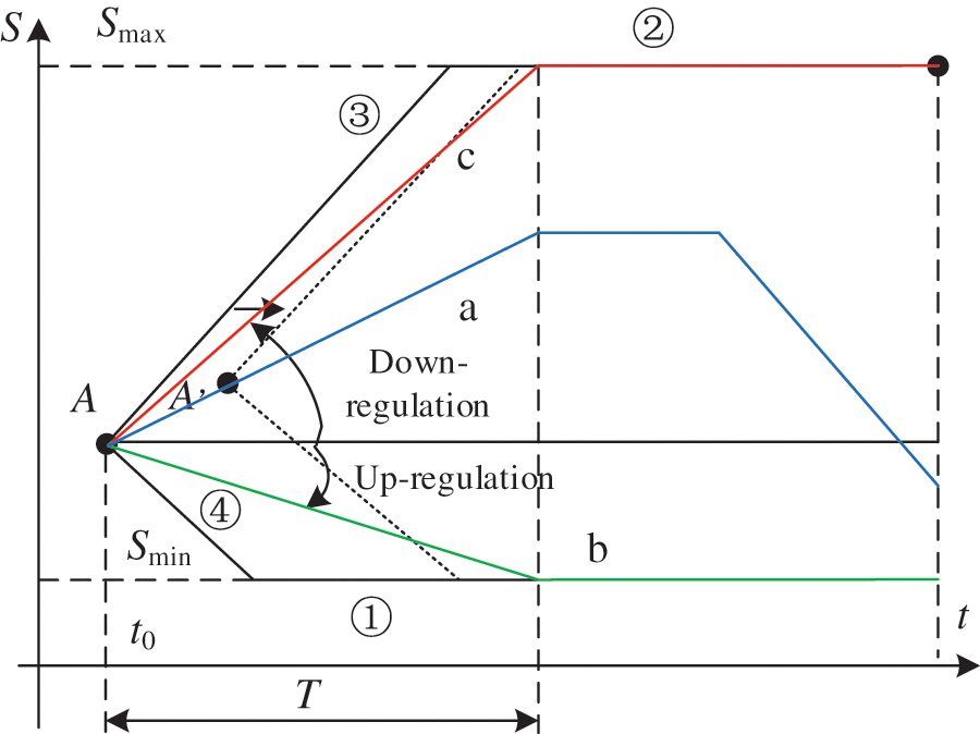
Figure 2: ESS operating range and constraints

When calculating the upward regulation capacity of the ESS, only constraints ① and ④ are likely to be triggered. Under such circumstances, the maximum discharging power of the ESS is determined as follows:

Pbatmin(t)=−min(Pbat,dmax,(Sbat(t0)−Sbat,min)Ebatηbat,d/T)(19)

Therefore, the upward regulation capacity of the ESS is determined as:

Pbat+(t)=min(Pbat(t)−Pbat,dmax,Pbatmin(t))(20)

When calculating the downward regulation capacity of the ESS, only constraints ② and ③ are likely to be triggered. Under such circumstances, the maximum charging power of the ESS is determined as follows:

Pbatmax(t)=min(Pbat,cmax,(Sbat,max−Sbat(t0))Ebat/(ηbat,cT))(21)

Therefore, the downward regulation capacity of the ESS is determined as:

Pbat−(t)=min(Pbat,cmax−Pbat(t),Pbatmax(t))(22)

where, Pbat+(t), Pbat−(t) represent the upward regulation ability and downward regulation ability of ESS, respectively.

2.4 GT Regulating Capacity

In the distribution system, GT with robust adjustment capabilities can swiftly react to load fluctuations, serving as a pivotal resource for the flexible supply of the distribution network [33]. The fast-regulating gas unit represented by GT participates in short-time scale regulation. During system power fluctuations, the GT can offer bidirectional adjustment capacity while operating under partial load conditions. The formula for calculating the adjustment capacity is as follows:

Pg+(t)=min[Rg+∗T,Pg,max−Pg(t)](23)

Pg−(t)=min[Rg−∗T,Pg(t)−Pg,min](24)

where, Pg+(t), Pg−(t) represent the upward regulation ability and downward regulation ability of GT, respectively; Pg(t) is the power of GT at time t; Rg+, Rg− represent the uphill and downhill climbing rates of GT, respectively; Pg,max, Pg,min respectively represent the maximum and minimum output of GT; The output state of GT at time t is related to the previous output state and the climbing power at that time scale, that is, Pg(t)=Pg(t−T)±ΔPg(t), ΔPg(t) is the changing output of GT at time t.

2.5 CL Regulating Capacity

The Controllable Load is a vital tool in achieving demand-side management. It employs various economic and technical methods to modify the load curve of the power system, enabling the load side to proactively respond to power fluctuations within the system. This means providing the system with adjustment capacity from the demand side [34]. In terms of flexibility, the Controllable Load can be regarded as a virtual standby power generation capacity resource on the load side. Its response time ranges from minutes to 10 min, and its fast response capability meets the demands of system load changes. It can participate in 15–60 min and >1 h medium and long-term scale adjustments. The size of its adjustment resources is primarily determined by the power load of the demand-side response implementing mechanism and its own maximum output change limit. The formula for calculating its adjustment capacity is as follows:

Pdr+(t)=min(PL,max−Pdr(t),0)(25)

Pdr−(t)=min(Pdr(t)−PL,min,0)(26)

where, Pdr+(t), Pdr−(t) represent the upward regulation ability and downward regulation ability of CL, respectively; Pdr(t) is the power of CL at time t; PL,max, PL,min respectively represent the maximum upward and downward output variation limits of CL itself, and their values are related to specific load characteristics.

3  Evaluation of the Regulation Capacity of the Distribution Station Area

(1) Adjustment Capability Boundary Index

Based on the analysis in Section 2, the upward and downward adjustment capabilities of the distribution panel area are calculated as follows:

UP(t)=∑g=1NGPg−(t)+∑e=1NESSPbat+(t)+∑d=1NDRPdr+(t)+∑ev=1NEVPev+(t)(27)

DP(t)=∑g=1NGPg+(t)+∑e=1NESSPbat−(t)+∑d=1NDRPdr−(t)+∑ev=1NEVPev−(t)(28)

where, UP(t), DP(t) represent the boundary indicators of the up and down adjustment ability of the distribution station area; NG, NESS, NDR, and NEV represent the number of installations for GT, ESS, CL, and EV, respectively; g, e, d, and ev are the indexes of GT, ESS, CL, and EV, respectively.

Using the above formula, the maximum upward and downward adjustment capabilities that can be provided in the distribution area at time t can be determined, as well as the transmission power for each line. Given that the power transmission of various resources is limited by the transmission capacity of the line, if the transmission power exceeds the maximum transmission capacity of the transmission line, it cannot ensure safe operation. Therefore, it is necessary to re-determine the adjustment capacity that the distribution station area can provide. Therefore, the adjustment capacity index is revised as follows:

Psys(t)=[Psys+(t),Psys−(t)](29)

Xsys+(t)=[ Pg−(t)​,Pbat+(t)​,Pdr+(t)​,Pev+(t) ]        g∈NG,bat∈NESS,dr∈NDR,ev∈NEV(30)

Xsys−(t)=[ Pg+(t)​,Pbat−(t)​,Pdr−(t)​,Pev−(t) ]        g∈NG,bat∈NESS,dr∈NDR,ev∈NEV(31)

Psys+(t)=min(Xsys+(t)​,Lk,type+(t)​,Lk,type−(t))         k∈Nl,type∈[ g,e,d,ev ](32)

Psys−(t)=min(Xsys−(t)​,Lk,type+(t)​,Lk,type−(t))        k∈Nl,type∈[ g,e,d,ev ](33)

where, Psys(t) are the adjustment range of the distribution station area; Xsys+(t), Xsys−(t) is the set of resource adjustment quantities for up and down adjustment in the distribution station area, respectively; Psys+(t), Psys−(t) represent the up and down regulation amount after considering the line capacity and adjusting the range of the distribution station area; Lk,type+(t), Lk,type−(t) are the maximum transmission capacity of the line up and down.

Eq. (29) represents the maximum regulating capacity range that the regulating resources can provide for the distribution panel area. Eqs. (30) and (31) represent the adjustable margins for the upward and downward adjustment capabilities of different resources, respectively. Eqs. (32) and (33) represent the correction of the adjustment resources’ upward and downward energy savings, taking into account the transmission capacity limitations of the line.

(2) Adjustment Capability Margin Index

According to the adjustment range provided by the adjustment resources, the actual upward margin and downward margin of the distribution panel area at time t can be calculated as follows:

UPsys(t)=Psys+(t)−Ppv(t)(34)

DPsys(t)=Ppv(t)−Psys−(t)(35)

where, UPsys(t), DPsys(t) represent the margin index of up and down adjustment capacity in the distribution station area, respectively; Ppv(t) is the power of PV at time t.

4  Cluster Optimization Operation Method of the Distribution Station Area

4.1 Distribution Station Area Cluster Division

4.1.1 Cluster Partition Index

The comprehensive performance indicators for distribution network cluster division encompass both structure and function [35,36]. Modularity serves as a common metric for evaluating network structure strength. In the context of distribution networks, the modularity index based on electrical distance is utilized to assess the strength of the power network structure. Active power balance refers to the ability to balance the active power of the source load within a cluster. In this paper, the module degree and active power balance index are integrated for the division of distribution network clusters, ensuring that the cluster division can effectively enhance the absorption capacity of PV and improve the regulation capacity of the distribution station area.

(1) Electrical Distance-Based Modularity Index

In the distribution network, the electrical distance weight is mainly determined by the voltage sensitivity between nodes. The relationship between the change in active power injection between two nodes and the change in node voltage can be expressed as:

Sij=∂Ui∂Pi=−1UN∑i=1min(i,j)Ri(36)

where, Sij is the element in the i row and j column of the sensitivity matrix; Ui represents the voltage at node i, Pj represents the power at node j, and ∂Ui/∂Pi indicate the change in voltage at node i caused by a unit change in power at node j; UN is the rated voltage of the distribution network nodes, which is taken as 12.66 kV; N is the number of system nodes; Ri represents the equivalent resistance between node i and node i−1.

The electrical distance between nodes is calculated using the Euclidean distance method based on node voltage sensitivity, specifically,

Xij=−log⁡|SijmaxSijj|(37)

dij=12[∑k=1N−1(Xik−Xjk)2](38)

where, maxSijj represents the maximum value among the elements in column j of the sensitivity matrix, and dij is the electrical distance between the edges connecting node i and node j.

The degree of electrical coupling between nodes is described using a modularity definition based on electrical distance weights, specifically,

ρ=12m∑i∑j(dij−kikj2m)δ(i,j)(39)

δ(i,j)={1i and j reside in the same partition0Other(40)

where, ρ is the modularity index; m is the sum of edge weights of all edges in the network; ki represents the sum of the weights of the edges connected to node i; kj represents the sum of the weights of the edges connected to node i.

(2) Active Power Balance Index

To represent the level of source-load matching within a cluster over a specific time scale, the active power balance index is defined based on net power as follows:

Pc(t)=Pload(t)−Ppv(t)(41)

φc=1−1T∑t=1T|Pc(t)maxPc(t)|(42)

φp=1Nc∑c∈Mφc(43)

where, Pc(t) represents the net power of cluster c at time; Nc represents the number of cluster partitions; M represents the collection of all clusters; φc represents the active power balance of cluster c; φp represents the overall active power balance of the network.

(3) Cluster Partition Method

In summary, the overall modular degree and active power balance degree of the system are integrated, and the system’s division mode is treated as the variable. To achieve maximum regional autonomous regulation within each cluster, a cluster division model is established based on the comprehensive division index.

maxφ=λ1ρ+λ2φp(44)

where, φ is the comprehensive division index; λ1 and λ2 represent the weight coefficients of different indicators, where λ1 + λ2 =1.

The larger the value of λ1, the better the cluster structure characteristics of the system; the larger the value of λ2, the higher the balance of flexibility resources in the system, and the better the flexibility characteristics of the cluster. In the absence of preferential requirements, averaging is the most conventional method that can reflect the relationship between targets. If one is more inclined to favor a particular target, the weight should be appropriately adjusted. If there are no specific requirements for the target, the method of averaging is the fairest and most conventional way to reflect the relationship between the targets. In this paper, to simultaneously take into account the system structure and power balance, the weights of the modularity index and active power balance index are set to 0.5 and 0.5, respectively.

4.1.2 Cluster Partitioning Method

As the comprehensive performance indicators of cluster partitioning involve both the structure and function of clusters, commonly used cluster partitioning algorithms cannot fully express the content of these indicators. Moreover, in networks with complex structures, changes in the number of clusters and the combinations of nodes within clusters have an impact on cluster performance. Genetic algorithms, through operations such as encoding, selection, crossover, and mutation, can effectively handle discrete variables and constraints. In the partitioning of distribution transformer areas, factors such as the connection relationships between nodes, electrical distances, and active power balance are discrete and constrained. Genetic algorithms can handle these discrete variables and constraints well, resulting in cluster partitioning outcomes that are in line with actual conditions.

When applied to cluster partitioning problems, genetic algorithms use the comprehensive cluster partitioning indicators as the fitness function and the cluster partitioning results as the optimization problem to be solved. To adapt to cluster partitioning, this article has improved the encoding method of genetic algorithms. Based on the adjacency matrix of the network, the chromosome is encoded in binary form. The 0–1 adjacency matrix is obtained based on the connection status of distribution network nodes. As shown in Fig. 3, the left figure is a simple network with 5 nodes, and the right figure is the adjacency matrix of this simple network. This encoding method not only ensures the connectivity of nodes but also greatly reduces the search range and time of genetic algorithms because each individual satisfies the connectivity requirement. At the same time, the genetic algorithm with this encoding method does not have the node merging process of general algorithms and uses a probability mechanism for iteration, which has strong search capabilities for irregular clusters. The specific cluster partitioning process is shown in Fig. 4.

Figure 3: Coding method of network adjacency matrix

Figure 4: Cluster division process based on genetic algorithm

4.2 Optimization Operation Method of the Distribution Station Area

Using the methods presented in Sections 2 and 3, we can determine the upward and downward adjustment amounts for each nod, as well as the cluster division result for the distribution station area. Based on this, we establish the evaluation model for the adjustment capacity of the station area, with the objective function being the lowest economic cost of the station area. We also take into account the operation constraints of the distribution network and the adjustment constraints of the adjustment resources.

4.2.1 Objective Function

The cost coefficients of different regulatory resources are determined based on actual construction and operation costs, including the power generation cost of GT, the ESS operating cost, the ESS regulatory cost, and the compensation cost of CL. The objective function is to minimize the adjustment cost of the station area:

minf=(fg,t+fbat,t+fev,t+fdr,t+fpv,t)(45)

{fg,t=∑t=1T∑g=1NGai+biPg(t)+cg,iPg(t)2fbat,t=∑t=1T∑e=1NESScbat|Pbat(t)|fev,t=∑t=1T∑ev=1NEVcv2gEev,totalCchange/Eev+cevPev(t)fdr,t=∑t=1T∑dr=1NDRcdrPdr(t)fpv.t=∑t=1T∑pv=1NPVcpv(Ppv,pre(t)−Ppv(t))(46)

where, fg,t, fbat,t, fev,t, fdr,t and fpv,t represent the generation cost, ESS operating cost, EV regulation cost, CL compensation cost, and PV abandonment cost of GT, respectively; a, b and cg are the operating cost coefficients of GT generator units; cbat is the operating cost per unit power of ESS; cv2g is the loss coefficient of the EV battery; cchange is the cost of replacing EV batteries; Eev,total is the total cycle charging and discharging capacity of the EV; cev is the cost coefficient specified by EV for the user; cdr is the cost coefficient of CL; cpv is the penalty cost coefficient for abandoning PV; Ppv,pre(t) represents the predicted maximum output of distributed PV at time t, and Npv is the number of PV installations.

4.2.2 Constraint Condition

Constraints include power balance constraint, line capacity constraint, operating safety constraint, and regulatory resources operating constraint.

1) Power Balance Constraint

∑g=1NGPg,i(t)+∑bat=1NESSPbat,i(t)+∑ev=1NEVPev,i(t)+∑dr=1NDRPdr,i(t)+∑pv=1NPVPpv,i(t)=Pload,i(t)(47)

where, Pload,i(t) is the load at time t.

2) Line Capacity Constraint

Pij,min≤Pij(t)≤Pij,max(48)

where, Pij,max, Pij,min represents the maximum and minimum transmission capacity of the line, respectively; Pij(t) is the transmission capacity of the line at time t.

3) Power Flow Constraint

{∑i:i→j(Pij(t)−RijLij(t))−Pj(t)=∑l:j→lPjl(t)∑i:i→j(Qij(t)−XijLij(t))−Qj(t)=∑l:j→lQjl(t)Uj2(t)=Ui2(t)−2(RijPij(t)+XijQij(t))+(Rij2+Xij2)Lij(t)(49)

Lij(t)=Pij2(t)+Qij2(t)Ui2(t)(50)

Pi(t)=Pload,i(t)−Ppv,i(t)(51)

Qi(t)=Qload,i(t)−Qpv,i(t)(52)

where, Pij(t) and Qij(t) are the active power and reactive power respectively flowing out from upstream node i to node j; Rij and Xij are the resistance and reactance of the line between node i and node j, respectively; Pi(t) is the net load active power of node i; Pload,i(t) is the load active power of node i; Ppv,i(t) is the active output power of the PV of node i; Qi(t) is the net load reactive power of node i; Qload,i(t) is the load reactive power of node i, and Qpv,i(t) is the reactive output power of the PV of node i.

Since Eq. (50) is a nonlinear equality constraint, which is non-convex and difficult to find the optimal solution, this nonlinear equality constraint is relaxed into an inequality constraint Eq. (52).

Lij(t)≥Pij2(t)+Qij2(t)Ui2(t)(53)

After replacing Eq. (50) with Eq. (53), the problem turns into a convex optimization problem, which is easier to solve.

4) Operating Safety Constraint

Umin2≤Ui2(t)≤Umax2(54)

where, Ui(t), Umin and Umax are the voltage, lower voltage limit, and upper voltage limit at the period node, respectively.

5) PV Power Generation Constraint

0≤Ppv(t)≤Ppv,pre(t)(55)

6) Regulatory Resources Operating Constraints

(1) Adjustment ability index constraint

DP(t)≤Pg(t)+Pbat(t)+Pev(t)+Pdr(t)+Ppv(t)≤UP(t)(56)

(2) EV constraint

In Section 2.2, the constraints of electric vehicles are analyzed, including their physical characteristics and user behavior constraints. Under these constraints, the adjustment capabilities of electric vehicles can vary, as described in Section 2.2.

(3) ESS constraint

As described in Section 2.3.

(4) GT constraint

Pg,min≤Pg,i(t)≤Pg,max(57)

(5) CL constraint

PL,min≤Pdr(t)≤PL,max(58)

5  Case Studies

5.1 Test System Parameters

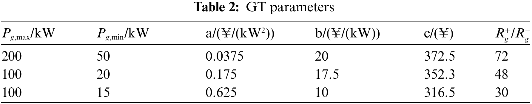
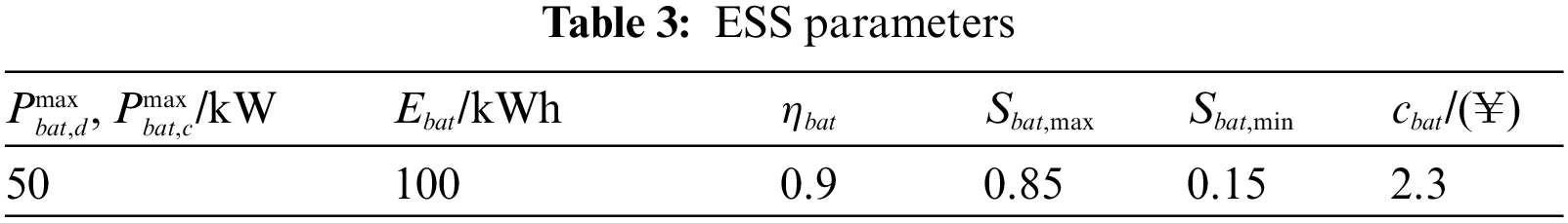
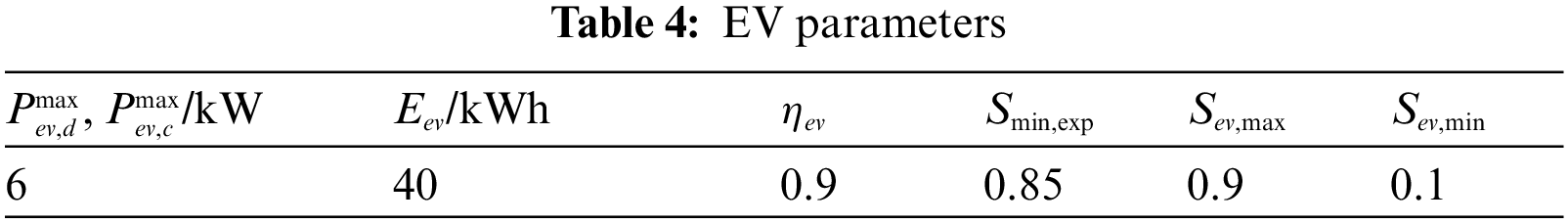
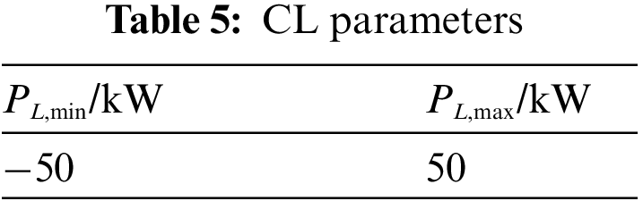
To validate the feasibility of the multi-spatiotemporal scale adjustment capability evaluation technology proposed in this paper, the IEEE33-node system has undergone enhancements. The reference voltage stands at 12.66 kV, and the reference power is set at 10 MW. Flexible resources are configured based on system requirements. As illustrated in Fig. 5, three GT are situated at nodes 2, 6, and 12, cumulatively boasting an installed capacity of 400 kW. Two ESS are installed at nodes 2 and 6, respectively, with a power output of 100 kW and a total capacity of 400 kWh. EV can be found at nodes 3, 6, 15, 22, 24, and 30, collectively contributing a power of 300 kW. CL are situated at nodes 5, 18, 22, 25, and 33, with an installed capacity of 150 kW. Additionally, six distributed PV units are installed at nodes 2, 6, 9, 14, 24, and 30, respectively, cumulatively generating a power of 500 kW. The system structure diagram of the calculation example is presented in Fig. 5. The parameters for the GT, ESS, EV, an CL are provided in Tables 2–5, respectively.

Figure 5: Schematic diagram of the exemplary system structure

5.2 Analysis of Cluster Division Results

On an hourly time scale, a day is divided into 24 time periods. The load active power demand and distributed PV active power prediction curves are shown in Fig. 6. It can be seen that the distributed PV predicted output is greater than the load demand from 10:00 to 15:00 during the day, and the load demand is greater than the PV predicted output at other times. There is no PV output from 01:00 to 05:00 and from 20:00 to 24:00. Due to the time-varying nature of load demand and distributed PV output within the distribution transformer area, the clustering results will change at different times of the day. However, in actual regulation, cluster partitioning is usually performed once a week. Therefore, to avoid dynamic changes in cluster partitioning, only the typical time scenario with the highest PV penetration in the distribution network, i.e., 13:00, is selected for cluster partitioning calculations. The weights of the cluster partitioning indicators can be selected based on the scheduling requirements of the dispatch center. Due to the inherent characteristics of the comprehensive performance indicators, different weight combinations will yield different results. In this example, considering generality, the weights of the modularity index and active power balance index are set to 0.5 and 0.5, respectively.

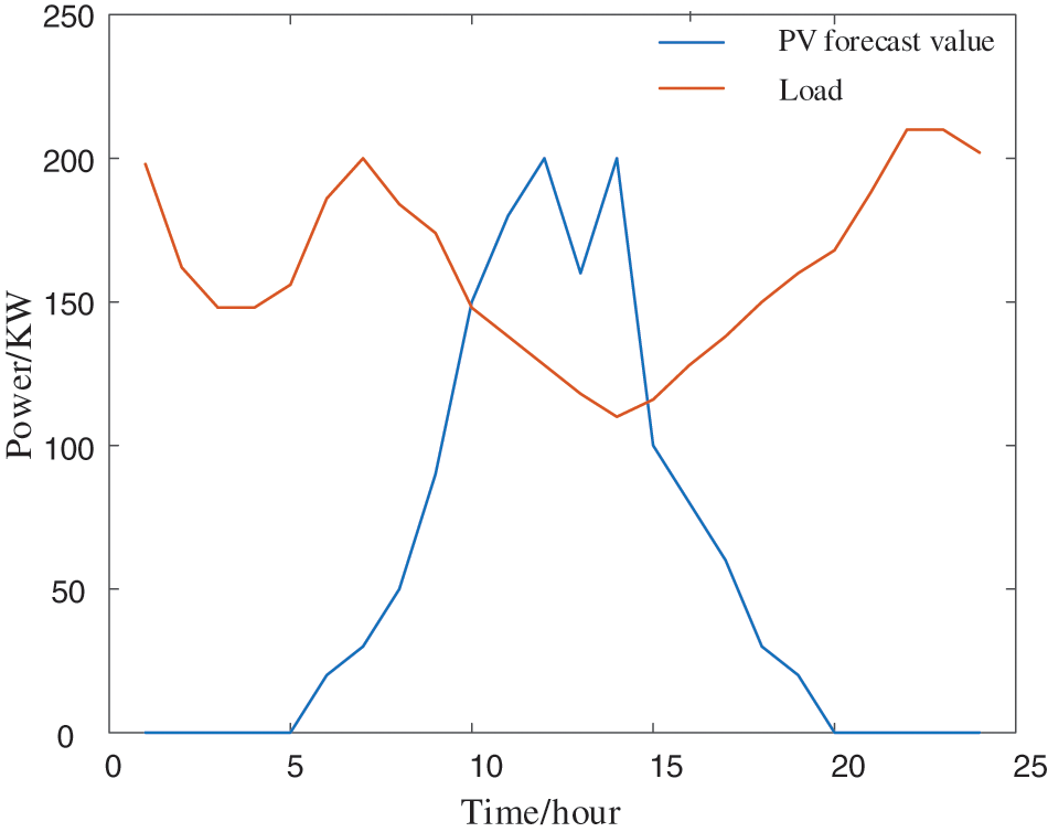
Figure 6: Load demand and PV forecast curve

When utilizing the genetic algorithm for clustering distributed PV stations within the distribution network, the maximum number of iterations is set to 800, the population size is set to 100, the crossover probability is set within the range of 0.2 to 0.6, and the mutation probability is set within the range of 0.05 to 0.50. To ensure convergence, the two optimal individuals following each iteration are disqualified from undergoing crossover and mutation operations.

Fig. 7 displays the variation curve of the comprehensive performance index as the number of clusters increases. It is evident that when the number of clusters is 3, the comprehensive performance index attains its maximum value of 0.10212. As analyzed in Section 3, when the number of clusters is 3, the cluster exhibits favorable structural characteristics and relatively superior power balance characteristics.

Figure 7: The index change curve is divided comprehensively

During cluster partitioning, the number of clusters can be set in the algorithm, and the optimization result represents the partitioning scenario with the highest comprehensive performance indicators under the current setting of cluster numbers. If the number of clusters is not set, the optimization result will be the partitioning scenario with the highest comprehensive performance indicators among all cluster partitioning combinations. In this example, the number of clusters is not set. Fig. 8 presents the cluster partitioning results, which show that the system is divided into three clusters. Each cluster has at least one PV node, ensuring that the adjustment resources within each cluster can accommodate PV power, improve the local PV accommodation rate, and ensure that the system’s flexible resource adjustment capabilities can be fully utilized.

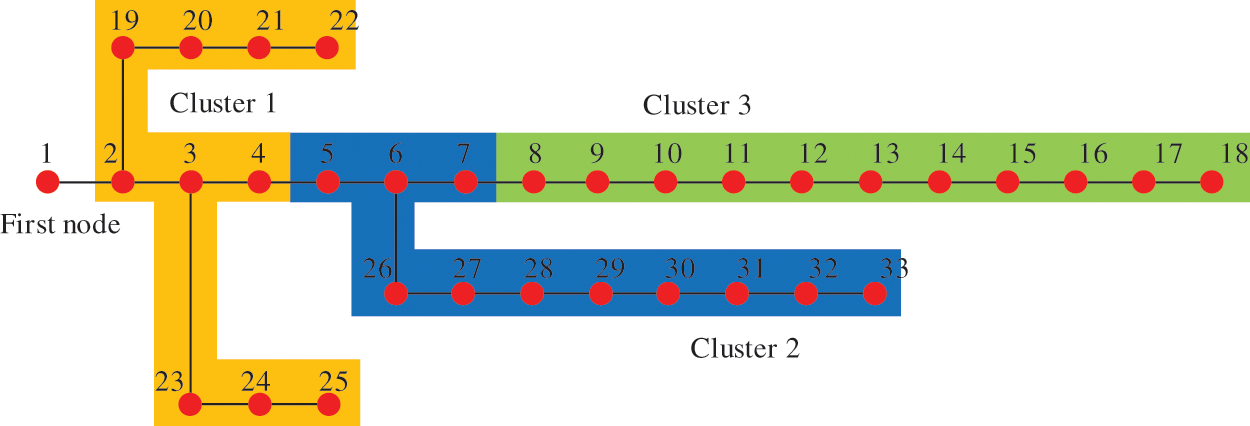
Figure 8: Cluster partition result

5.3 Analysis of Adjustment Ability Evaluation Results

To validate the effectiveness of the adjustment capacity assessment technique proposed in this paper, two schemes are compared and analyzed as follows:

Case 1: Traditional evaluation techniques focus on assessing the flexibility of regulation resources without considering cluster partitioning and line transmission capacity.

Case 2: The evaluation technique proposed in this article assesses the regulation capabilities provided by the feasible region of regulation resources, taking into account cluster partitioning and line transmission capacity assessment techniques.

A comparison of the optimization results, as shown in Table 6, reveals that when cluster partitioning is not considered, there are no constraints on power exchange between clusters. Under a higher setting of curtailed PV power costs, the curtailment rate is zero. However, increased power transmission leads to higher network losses, resulting in relatively lower operational costs for the distribution system.

A comparison of the network loss in the distribution system is shown in Fig. 9. It can be observed that during the period from 12:00 to 14:00 when the distributed PV penetration rate in the system is relatively high, the network loss in the distribution system considering cluster partitioning is significantly lower than that without considering cluster partitioning. This is because after cluster partitioning, the constraints on power exchange between clusters limit the transmission of PV active power to other clusters, i.e., to remote distribution transformer areas, thereby reducing the power flow on the branches between clusters and thus reducing system network losses. As can be seen from Table 6, while cluster partitioning significantly reduces system network losses, it only brings about a small increase in costs and a slight phenomenon of PV curtailment. Figs. 10 and 11 further demonstrate that cluster partitioning not only greatly reduces system network losses but also enhances the adjustment capabilities of distribution transformer areas. This is because the constraints on power exchange between clusters limit the transfer of adjustment resources within each cluster to other clusters, thus increasing the adjustment range of each resource and subsequently enhancing the adjustment capabilities of transformer areas within each cluster.

Figure 9: Power distribution system network loss

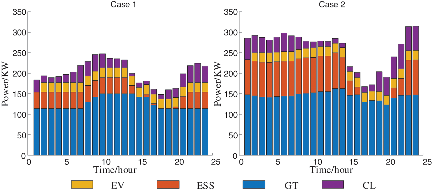
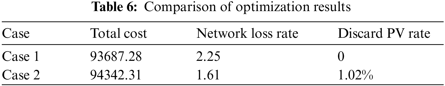
Figure 10: Case 1 and Case 2 adjust the upward adjustment ability of resources

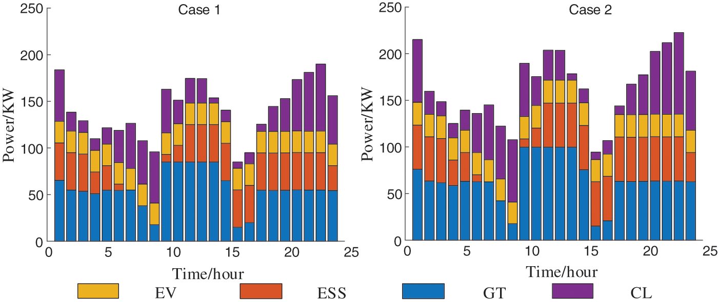
Figure 11: Case 1 and Case 2 adjust the downward adjustment ability of resources

In terms of the line’s support capacity for regulation capacity, Fig. 12 presents the regulation capacity of the distribution area under two evaluation schemes. Case 1 does not consider line capacity, and Case 2 considers line capacity. To clearly communicate the results, the upward and downward regulation capacity is expressed in absolute value. It is observed that the upward and downward adjustment capabilities of both evaluation schemes are greater than zero, indicating that the supply of adjusted resources meets the load demand and flexible supply and demand can be balanced. This is because various regulation resources are involved in regulation, with GT and ESS demonstrating fast dynamic response and good bidirectional regulation ability. When considering the line transmission capacity, it can be seen that the adjustment capacity of the distribution area will be reduced. Conversely, if the line transmission capacity is not considered, the calculated adjustment capacity may be excessively large in some periods, leading to the abandonment of light issues. When focusing on the absorption rate of distributed PV, efforts are made to adjust resources and power transmission within the cluster to absorb PV as much as possible. However, this may exceed transmission line capacity limits, resulting in line-over-limit problems. When safety is emphasized, part of the regulation capacity of the distribution area will be reduced. Therefore, considering the line capacity issue, the scope of regulation capacity can be more accurately determined, enabling the regulation capacity index to evaluate regulation capacity more effectively and guide scheduling.

Figure 12: The adjustment capacity of the distribution station area

5.4 Analysis of Adjustment Ability Evaluation Results

Fig. 13 shows the load of distributed PV, EC, GT, ESS, CL, and other types of flexible resources in each period of a typical day.

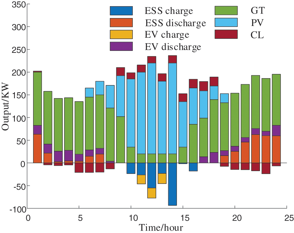
Figure 13: Distributed PV and output results of various regulatory resources

The voltage output of distributed PV and the output of each regulatory resource are analyzed as follows:

As shown in Fig. 13, ESS and GT possess strong time-scale adjustment capabilities, with a certain amount of power adjustment during peak and low PV output periods. The adjustment capacity of CL and EV is relatively small, and their time adjustment range is also relatively narrow due to their load constraints and user constraints.

The cluster division of the distribution station area can minimize the transmission of PV active power to other distribution station areas, utilizing the adjustment resources within the distribution station area to meet load demand and PV consumption, which can reduce power losses on the distribution station area’s lines. Excessive PV output beyond the regulating capacity of each regulatory resource and line capacity is discarded.

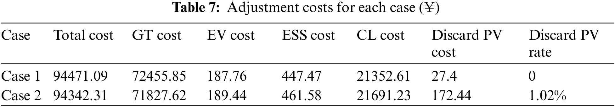
As Fig. 14 reveals, the peak period of PV power generation occurs between 12:00 and 14:00, during which the distributed PV output within the station area exceeds the load demand. Under Case 1, when PV power generation rises, GT prioritizes reducing power generation to increase PV consumption, narrowing GT’s adjustment range, as shown in Fig. 15. In Case 2, ESS prefers charging due to its high efficiency and low-cost factor. When storage capacity is limited, EV and CL become involved in adjustment. When PV power generation drops significantly, ESS discharge supplements partial energy shortages and reduces GT power generation. In Case 2, the operating cost of regulation resources in the distribution station area is considered. This increases the adjustment costs of ESS, EV, and CL but reduces the cost loss of GT, ultimately reducing the total operating cost, as outlined in Table 7. Furthermore, the light rejection rate in Scenario 2 is 1.02%, which remains minimal for practical projects. Additionally, when evaluating the regulation capacity of the distribution station area, comprehensively considering the operation cost of regulation resources better ensures economic operation, safety, and stability of the distribution network compared to the additional economic costs caused by distributed PV unified dispatch of the distribution network and real-time efficient regulation.

Figure 14: PV uptake of Case 1 and Case 2

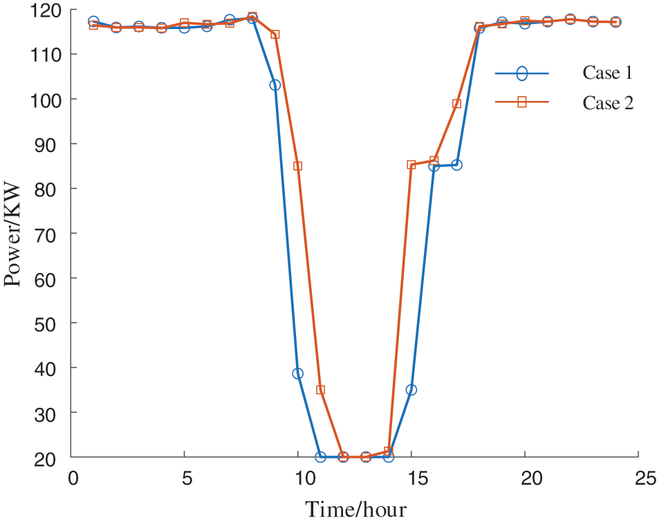
Figure 15: GT output for Case 1 and Case 2

6  Conclusion

This paper introduces a multi-temporal scale adjustment capability assessment technique for distributed PV distribution networks, taking into account diverse geographical locations, coverage areas, and response capabilities. The main conclusions are summarized as follows:

1) This study takes into account the adjustment characteristics of various resources in distribution networks and establishes a resource adjustment model for distribution networks. This model can quantify the maximum adjustable range of resources, both upwards and downwards. Furthermore, by considering the constraints of line transmission capacity, it reflects the support capability of lines in meeting adjustment demands. This approach can alleviate the issue of unavailable adjustment capabilities, reduce line congestion and load shedding in practical applications, and provide a reference for flexible assessment of distribution networks.

2) Based on modularity indicators related to electrical distance and active power balance indicators, this paper proposes a cluster division method for distributed PV distribution networks using an improved genetic algorithm. This method can reduce network losses and enhance the adjustment capabilities of distribution networks. It not only facilitates the local consumption of PV energy within distribution networks but also minimizes unnecessary resource waste and improves the overall operational efficiency of the power system.

3) This paper considers the adjustment costs of various resources in distribution networks and presents an economic optimization model for distribution networks. By incorporating economic considerations into the assessment of adjustment capabilities, it aims to reduce overall operational costs. The abandonment rate of PV energy is merely 1.02%, which is relatively low for engineering applications, demonstrating its superior economic viability and flexibility. Electric power departments can rely on the guidance of this optimization model to formulate more reasonable resource scheduling plans, providing a reference for resource allocation and enhancing the overall economic benefits of distribution networks.

Acknowledgement: This paper is supported by the Science and Technology Project of the Headquarters of the State Grid Corporation (Research and Application Project of Collaborative Optimization Control Technology for Distribution Station Area for High Proportion Distributed PV Consumption, 4000-202318079A-1-1-ZN).

Funding Statement: This research was funded by the “Research and Application Project of Collaborative Optimization Control Technology for Distribution Station Area for High Proportion Distributed PV Consumption (4000-202318079A-1-1-ZN)” of the Headquarters of the State Grid Corporation.

Author Contributions: The authors confirm contribution to the paper as follows: Study conception and design: Yuchen Hao, Yingqi Liao, Fang Liang, Jiaxin Qiao; data collection: Yuchen Hao, Yingqi Liao, Fang Liang; analysis and interpretation of results: Jing Bian, Jiaxin Qiao; draft manuscript preparation: Jing Bian, Jiaxin Qiao. All authors reviewed the results and approved the final version of the manuscript.

Availability of Data and Materials: Data not available due to [ethical/legal/commercial] restrictions. Due to the nature of this research, participants of this study did not agree for their data to be shared publicly, so supporting data is not available.

Conflicts of Interest: The authors declare that they have no conflicts of interest to report regarding the present study.

References

1. G. H. Tong, “Construction of smart energy system based on dual carbon goal,” (in ChineseSmart Power, vol. 49, no. 5, pp. 1–6, May 2021. [Google Scholar]

2. J. C. Zhang, M. Li, Z. W. Liu, J. Tan, Y. G. Tao, and T. L. Luo, “An evaluation method for multi-type flexible resource regulation capability on the user side of distribution networks,” (in ChineseElectric Power, vol. 56, no. 9, pp. 96–103, Dec. 2023. [Google Scholar]

3. C. Chen et al., “Two-staged generation-grid-load-energy storage interactive optimization operation strategy for promotion of distributed PV consumption,” (in ChinesePower Syst. Technol., vol. 46, no. 10, pp. 3786–3799, Aug. 2022. [Google Scholar]

4. B. Mohandes, M. S. E. Moursi, N. Hatziargyroun, and S. E. Khatib, “A review of power system flexibility with high penetration of renewables,” IEEE Trans. Power Syst., vol. 34, no. 4, pp. 3140–3155, Feb. 2019. [Google Scholar]

5. J. Y. Wen, B. Zhou, and L. C. Wei, “Preliminary study on an energy storage grid for future power system in China,” (in ChinesePower Syst. Prot. Control, vol. 50, no. 7, pp. 1–10, Apr. 2022. [Google Scholar]

6. Z. Y. Wu, M. Zhou, J. X. Wang, W. Y. Tang, B. Yuan and G. Y. Li, “Review on market mechanism to enhance the flexibility of power system under the dual-carbon target,” (in ChineseProc. CSEE, vol. 42, no. 2, pp. 7746–7764, Jan. 2022. [Google Scholar]

7. M. Nayeripour, H. Fallahzadeh-Abarghouei, E. Waffenschmidt, and S. Hasanvand, “Coordinated online voltage management of distributed generation using network partitioning,” Elect. Power Syst. Res., vol. 141, pp. 202–209, Nov. 2016. [Google Scholar]

8. D. Hu, M. Ding, R. Bi, X. F. Liu, and X. T. Rong, “Sizing and placement of distributed generation and energy storage for a largescale distribution network employing cluster partitioning,” J. Renew. Sustain. Energy, vol. 10, no. 2, Article No. 025301, Dec. 2018. [Google Scholar]

9. E. S. Du, N. Zhang, C. Q. Kang, and X. Qing, “A high-efficiency network-constrained clustered unit commitment model for power system planning studies,” IEEE Trans. Power Syst., vol. 34, no. 4, pp. 2498–2508, Nov. 2018. [Google Scholar]

10. B. Xiao et al., “Power source flexibility margin quantification method for multi-energy power system based on blind number theory,” CSEE J. Power Energy Syst., vol. 9, no. 6, pp. 2321, Jan. 2024. [Google Scholar]

11. R. Bi, X. F. Lui, M. Ding, H. Fang, J. J. Zhang and F. Chen, “Renewable energy generation cluster partition method aiming at improving accommodation capacity,” (in ChineseProc. CSEE, vol. 39, no. 22, pp. 6583–6592, Nov. 2019. [Google Scholar]

12. W. X. Sheng et al., “Key techniques and engineering practice of distributed renewable generation clusters integration,” (in ChineseProc. CSEE, vol. 39, no. 8, pp. 2175–2186, Apr. 2019. [Google Scholar]

13. B. Zhao, Z. C. Xu, and C. Xu, “Network partition-based zonal voltage control for distribution networks with distributed PV systems,” IEEE Trans. Smart Grid, vol. 9, no. 5, pp. 4087–4098, Sep. 2018. [Google Scholar]

14. Y. Y. Chai, L. Guo, C. S. Wang, Z. Z. Zhao, X. F. Du and J. Pan, “Network partition and voltage coordination control for distribution networks with high penetration of distributed PV units,” IEEE Trans. Power Syst., vol. 33, no. 3, pp. 3396–3407, May 2018. [Google Scholar]

15. H. Bitara and S. Rahman, “Reducing curtailed wind energy through energy storage and demand response,” IEEE Trans. Sustain. Energy, vol. 9, no. 1, pp. 228–236, Jan. 2018. [Google Scholar]

16. Z. H. Li et al., “Assessment of renewable energy accommodation based on system flexibility analysis,” (in ChinesePower Syst. Technol., vol. 41, no. 7, pp. 2187–2194, Jun. 2017. [Google Scholar]

17. Z. X. Lu, H. B. Li, and Y. Qiao, “Flexibility evaluation and supply/demand balance principle of power system with high-penetration renewable electricity,” (in ChineseProc. CSEE, vol. 37, no. 1, pp. 9–19, Jan. 2017. [Google Scholar]

18. E. Lannoye, D. Flynn, and M. O’Malley, “Evaluation of power system flexibility,” IEEE Trans. Power Syst., vol. 27, no. 2, pp. 922–931, May 2012. [Google Scholar]

19. J. Ma, V. Silva, R. Belhomme, D. S. Kirschen, and L. F. Ochoa, “Evaluating and planning flexibility in sustainable power systems,” IEEE Trans. Sustain. Energy, vol. 4, no. 1, pp. 200–209, Jan. 2013. [Google Scholar]

20. Y. H. Zhou et al., “Small-signal stability assessment of heterogeneous grid-following converter power systems based on grid strength analysis,” IEEE Trans. Power Syst., vol. 38, no. 3, pp. 2566–2578, May 2023. [Google Scholar]

21. L. Saarinen and K. Tokimatsu, “Flexibility metrics for analysis of power system transition-a case study of Japan and Sweden,” Renew. Energy, vol. 170, pp. 764–772, Jun. 2021. [Google Scholar]

22. T. Heggarty, J. Y. Bourmaud, R. Girard, and G. Kariniotakis, “Multi-temporal assessment of power system flexibility requirement,” Appl. Energy, vol. 238, pp. 1327–1336, Mar. 2019. [Google Scholar]

23. T. Heggarty, J. Y. Bourmaud, R. Girard, and G. Kariniotakis, “Quantifying power system flexibility provision,” Appl. Energy, vol. 279, pp. 1–12, Dec. 2020. [Google Scholar]

24. Y. K. Kim, G. S. Lee, J. S. Yoon, and S. I. Moon, “Evaluation for maximum allowable capacity of renewable energy source considering AC system strength measures,” IEEE Trans. Sustain. Energy, vol. 13, no. 2, pp. 1123–1134, Apr. 2022. [Google Scholar]

25. E. Lannoye, D. Flynn, and M. O’Malley, “Transmission, variable generation, and power system flexibility,” IEEE Trans. Power Syst., vol. 30, no. 1, pp. 57–66, Jan. 2015. [Google Scholar]

26. Z. Y. Lin, H. Q. Li, Y. C. Su, and J. Gou, “Evaluation and expansion planning method of a power system considering flexible carrying capacity,” (in ChinesePower Syst. Prot. Control, vol. 49, no. 5, pp. 46–57, Mar. 2021. [Google Scholar]

27. H. H. Chen, X. Fang, R. F. Zhang, T. Jiang, G. Q. Li and F. X. Li, “Available transfer capability evaluation in a deregulated electricity market considering correlated wind power,” IET Gen., Trans. Distrib., vol. 12, no. 1, pp. 53–61, Jan. 2018. [Google Scholar]

28. J. R. Xue, X. H. Shi, C. Wang, Y. J. Cao, and H. X. Zhang, “Online evaluation of emergency power regulation capability for virtual power plants considering physical characteristics and user behavior constraints,” (in ChineseProc. CSEE, vol. 43, no. 8, pp. 2906–2921, Dec. 2022. [Google Scholar]

29. C. Zhang, J. B. Greenblatt, P. MacDougall, S. Saxena, and A. J. Prabhakar, “Quantifying the benefits of electric vehicles on the future electricity grid in the mid western United States,” Appl. Energy, vol. 270, Article No. 115174, Jul. 2020. [Google Scholar]

30. M. Asensio and J. Contreras, “Stochastic unit commitment in isolated systems with renewable penetration under CVaR assessment,” IEEE Trans. Smart Grid, vol. 7, no. 3, pp. 1356–1367, May 2016. [Google Scholar]

31. P. Wang, D. Wu, and K. Kalsi, “Flexibility estimation and control of thermostatically controlled loads with lock time for regulation service,” IEEE Trans. Smart Grid, vol. 11, no. 4, pp. 3221–3230, Jul. 2020. [Google Scholar]

32. G. Wenze, M. Negrete-Pincetic, D. E. Olivares, J. MacDonald, and D. S. Callaway, “Real-time charging strategies for an electric vehicle aggregator to provide ancillary services,” IEEE Trans. Smart Grid, vol. 9, no. 5, pp. 5141–5151, Sep. 2018. [Google Scholar]

33. A. Roos and T. F. Bolkesjo, “Value of demand flexibility on spot and reserve electricity markets in future power system with increased shares of variable renewable energy,” Energy, vol. 144, pp. 201–217, Feb. 2018. [Google Scholar]

34. A. O. Salau, Y. W. Gebru, and D. Bitew, “Optimal network reconfiguration for power loss minimization and voltage profile enhancement in distribution systems,” Elect. Power Syst. Res., vol. 6, no. 6, pp. 1–8, Jun. 2020. [Google Scholar]

35. A. Dadkhah, B. Vahidi, M. Shafie-khah, and J. P. S. Catalao, “Power system flexibility improvement with a focus on demand response and wind power variability,” IET Renew. Power Gener., vol. 14, no. 6, pp. 1095–1103, Apr. 2020. [Google Scholar]

36. E. Cotilla-Sanchez, P. D. H. Hines, C. Barrows, S. Blumsack, and M. Patel, “Multi-attribute partitioning of power networks based on electrical distance,” IEEE Trans. Power Syst., vol. 28, no. 4, pp. 4979–4987, Nov. 2013. [Google Scholar]