
 Submit a Paper
 Propose a Special lssue
 Open Access
ARTICLE

Production Capacity Prediction Method of Shale Oil Based on Machine Learning Combination Model
1 Petroleum Engineering Technology Research Institute of Shengli Oilfield, SINOPEC, Dongying, 257000, China
2 Postdoctoral Scientific Research Working Station of Shengli Oilfield, SINOPEC, Dongying, 257000, China
* Corresponding Author: Mingjing Lu. Email:
(This article belongs to the Special Issue: Integrated Geology-Engineering Simulation and Optimizationfor Unconventional Oil and Gas Reservoirs)
Energy Engineering 2024, 121(8), 2167-2190. https://doi.org/10.32604/ee.2024.049430
Received 07 January 2024; Accepted 22 March 2024; Issue published 19 July 2024
 View Full Text
 Download PDF
Abstract
The production capacity of shale oil reservoirs after hydraulic fracturing is influenced by a complex interplay involving geological characteristics, engineering quality, and well conditions. These relationships, nonlinear in nature, pose challenges for accurate description through physical models. While field data provides insights into real-world effects, its limited volume and quality restrict its utility. Complementing this, numerical simulation models offer effective support. To harness the strengths of both data-driven and model-driven approaches, this study established a shale oil production capacity prediction model based on a machine learning combination model. Leveraging fracturing development data from 236 wells in the field, a data-driven method employing the random forest algorithm is implemented to identify the main controlling factors for different types of shale oil reservoirs. Through the combination model integrating support vector machine (SVM) algorithm and back propagation neural network (BPNN), a model-driven shale oil production capacity prediction model is developed, capable of swiftly responding to shale oil development performance under varying geological, fluid, and well conditions. The results of numerical experiments show that the proposed method demonstrates a notable enhancement in R by 22.5% and 5.8% compared to singular machine learning models like SVM and BPNN, showcasing its superior precision in predicting shale oil production capacity across diverse datasets.Keywords
Nomenclature
| Partition variable | |
| Corresponding threshold | |
| Corresponding loss function | |
| Mean of y for cases where the j-th variable does not exceed | |
| Mean of y where the j-th variable surpasses | |
| OOB baseline error for the t-th CART | |
| Resultant OOB error | |
| Sum of all the values of the decrease of the accuracy | |
| Bandwidth of the kernel | |
| Reciprocal of the influence radius | |
| Penalty factor | |
| Relative error of the i single machine learning model | |
| Flow velocity | |
| Relative permeability | |
| Permeability | |
| Viscosity | |
| Threshold pressure gradient | |
| Potential gradient | |
| Initial permeability | |
| Initial reservoir pressure | |
| Stress sensitivity coefficient | |
| Flow velocities of the oil, gas, and water phases | |
| Densities of oil and dissolved gas components within the oil phase | |
| Densities of the gas and water phases | |
| Source or sink terms for the oil, gas, and water components | |
| Porosity | |
| Saturation levels of the oil, gas, and water phases | |
| Pressures of the oil, gas, and water phases | |
| Capillary forces between oil-water and oil-gas | |
| Standardized data | |
| Original data | |
| Standard deviation of the data | |
| Mean of the data | |
| Actual and predicted value | |
| Mean of actual values | |
| Size of actual values within the validation set | |
| Predictions of the base learners | |
| Weights attributed to different base learners |
The prediction and evaluation of horizontal well production capacity is the key to the rational and effective development of shale oil reservoirs [1,2]. Shale reservoirs have poor physical properties and complex pore and throat structures, and the economic benefits of conventional straight well development are poor, and the multi-stage fracturing technology of horizontal wells is mostly used to improve production [3,4]. Due to the complex distribution and mutual interference of fracture network after volumetric fracturing, and the complex mapping relationship between fracture network structure, fracturing parameters, and production, the traditional empirical formula method and mathematical analysis method generally have large errors in shale oil production capacity prediction, and have weak adaptability to new data, making it difficult to promote. At present, there are many methods for conventional reservoir production capacity prediction in reservoir engineering, which mainly use well-system test data, including formation pressure, bottom-hole flow pressure, and test production [5]. Regarding the production capacity prediction methods of shale oil reservoirs, previous researchers have done a lot of research and achieved some results, which can be broadly classified into two categories [6–9]: One category is the reservoir engineering methods, mainly based on non-Darcy seepage flow, to derive production capacity formulas applicable to the consideration of different shale oil development mechanism [10]. The other category is the artificial intelligence method, which mainly uses the support vector machine, neural network, and other machine learning methods to deal with the geological parameters and field production parameters of the shale oil reservoir, so as to establish the production capacity prediction model by analyzing the potential patterns within a large amount of data [11–13]. Compared with traditional production capacity prediction methods, machine learning methods not only shorten the modeling cycle and accelerate the computational speed but also have better scalability [14,15]. Therefore, it is of great theoretical significance to establish a production capacity prediction model for shale oil reservoirs based on machine learning on the basis of clarifying the main controlling factors affecting the shale oil production capacity, which can further optimize the fracturing parameters, improve the design level of fracturing technology, and improve the development effect.
In the evaluation process of shale oil production capacity, understanding the extent of influence and interrelationships among various factors is crucial [16]. However, within these factors, inevitable correlations or overlaps among certain parameters may affect the final evaluation outcomes. Consequently, numerous scholars have undertaken main controlling factor screening studies in the petroleum engineering domain [17,18]. Zoveidavianpoor et al. [19] employed Gaussian distribution membership functions, considering seven geological parameters such as permeability and skin coefficient as input variables. They determined weights based on expert knowledge and conducted fuzzy comprehensive evaluations of candidate fracturing wells. Davarpanah et al. [20] utilized the fuzzy analytic hierarchy process and TOPSIS (technique for order preference by similarity to ideal solution) to analyze and compare five indicators affecting hydraulic fracturing effectiveness. The weights for each factor were derived from expert experience. Gou et al. [21] conducted a grey cluster analysis to screen and retain geological and engineering parameters most significantly correlated with production. These selected parameters were used as input variables to establish a model for assessing the enhanced production potential of fractured wells [22]. However, existing methodologies have yet to effectively integrate the reliability of field data with the supplemental aspects of numerical simulation data [23]. Consequently, they fail to rationalize the fusion and dimensionality reduction of data features, unable to ensure each factor contributes unique information to the capacity assessment rather than duplication or excessive layering.
Machine learning (ML) excels in extracting information from high-dimensional, complex data, playing a significant role in predicting reservoir production capacity automatically in supervised or unsupervised modes [24]. Extensive studies by scholars have shown the superiority of ML algorithms over traditional prediction methods like logistic regression in forecasting reservoir production capacity [25,26]. Zhou et al. [27] combined principal component analysis, cluster analysis, and regression analysis to compute shale gas production in specific regions based on variables such as hydraulic fracture count, well deviation, vertical depth, and fracturing fluid. Lolon et al. [28] employed three multivariate statistical models to assess the correlation between drilling parameters and production, highlighting the technical variables (total fracturing fluid volume and proppant dosage during hydraulic fracturing) that notably affect tight oil reservoir production. Additionally, Mohaghegh et al. [29] proposed a shale gas analysis concept based on big data, constructing a production capacity prediction model using artificial neural networks. They utilized this model to develop templates correlating production capacity with fracturing construction parameters. Lu et al. [30] proposed a computational framework for shale oil production prediction and fracturing parameters optimization that couples deep neural network (DNN) and particle swarm optimization (PSO). The generalization ability of DNN is verified by the accurate prediction performance of 4 cases with extreme parameters. Mahzari et al. [31] developed a deep learning algorithm to use the pertinent production profiles such as oil rate, gas oil ratio (GOR), water oil ratio (WOR) to train the shale oil production prediction model. Hui et al. [32] established an integrated machine learning-based approach to determine the major determinants regulating shale gas productivity through the integration of reservoir features and shale production. The aforementioned machine learning methods each have their own advantages and drawbacks. For instance, the Random Forest method is capable of handling various types of features, including missing values and categorical features. However, due to its ensemble nature based on decision trees, it may lack flexibility and struggle to effectively capture certain complex data patterns. XGBoost algorithm exhibits strong predictive capabilities and often achieves good performance. Nonetheless, it may encounter overfitting issues necessitating additional methods such as regularization for mitigation. The Support Vector Machine method performs well with small sample datasets but exhibits longer training times with large-scale datasets. The Back Propagation Neural Network can learn complex nonlinear relationships, making it suitable for high-dimensional and large-scale datasets. However, it is prone to getting trapped in local optima during training, thus requiring careful selection of optimization algorithms and initialization parameters. Given the strengths and limitations of different ML methods, it is essential to choose an appropriate ML approach tailored to the characteristics of the data samples at hand. While these machine learning and deep learning methods rely on a singular model, introducing uncertainties in model selection [33]. However, shale oil production capacity is influenced by multiple factors, making it challenging for a single ML-based prediction approach to meet the requirements of precision and accuracy necessary for intricate development. Therefore, adhering to the principle of leveraging complementary strengths, a combination model is constructed by integrating the advantages of various prediction models and using appropriate weighting combination methods. This model aims to effectively guide intelligent production forecasting in the implementation of volume fracturing in horizontal wells in shale oil reservoirs.
This study utilizes the random forest method to assess the main controlling factors influencing shale oil production capacity across various reservoirs. It leverages drilling, fracturing, and well-testing data from 236 horizontal wells subjected to volume fracturing in the R1 and R2 reservoirs. Additionally, it constructs a sample set for predicting production capacity through numerical simulation models of shale oil reservoir seepage. Employing a machine learning combination model with support vector machine and BP neural network as base learners, the study establishes a prediction model specifically targeting accurate estimates of production capacity for fractured horizontal wells.
Machine learning algorithms, particularly Random Forest (RF), have increasingly been applied to evaluate the main controlling factors of shale oil production capacity. This algorithm, a key representative of bagging ensemble methods, efficiently handles typical datasets in shale oil production capacity analysis, offering extensive application in feature screening and prediction.
The dataset in question, designated as X = {X1, X2, ..., XN}, where each Xi = {xi,1, xi,2, ..., xi,M}, comprises N instances, each constituted by M variables. The output dataset is denoted as Y = {Y1,Y2, ...,YN}. Given a partition variable
where
Upon finalization of the RF model, it becomes feasible to calculate the significance or influence of each input variable. During the individual CART training, N instances are randomly selected with replacement from the dataset, leaving a subset of unchosen instances known as Out of Bag (OOB) samples. Following training, these OOB samples serve to evaluate the impact of input variables on the RF model. Assuming the RF model incorporates T CARTs, and defining the OOB baseline error for the t-th CART as
Aggregating the decrements in accuracy for the j-th variable across all CARTs yields the mean decrement:
This mean is normalized to represent the variable’s contribution to the model’s performance regarding corrosion, formulated as:
where
Through the computation of the Gini coefficient for each decision tree node, RF efficiently assesses the relative significance of different factors, facilitating informed decision-making processes. Its ability to mitigate overfitting and accommodate diverse data types makes it an ideal tool for identifying the main controlling factors influencing shale oil production capacity.
Support Vector Machine (SVM) is a generalized linear classifier and regressor [35]. SVM solves classification and regression problems by supervised learning on data. The decision boundary is the maximal margin hyperplane that the training data has. SVMs work with the goal of classifying this training data into as many different regions as possible and maximizing the distance from the nearest data point to the hyperplane to that hyperplane. The process of training the SVM is obtained by solving a convex quadratic programming problem whose solution can be expressed as a linear combination of support vectors. In conclusion, SVM is an effective classifier and regressor and has good generalization ability for dealing with linear and nonlinear differentiable datasets.
In regression analysis, after mapping samples into higher dimensions, it is essential to identify a separating line (hyperplane) that minimizes the distance between two sample points furthest apart (perpendicular to the hyperplane). This approach aims to predict sample outcomes based on their proximity to the hyperplane. SVM employs the Radial Basis Function (RBF) kernel to map samples into higher dimensions, following the formula:
where
During model training, the model uses a loss function with L2 regularization (which reduces overfitting):
where
The Back Propagation Neural Network (BPNN) stands as one of the fundamental models in machine learning [36]. It comprises an input layer, hidden layers, and an output layer, with signal propagation occurring between layers through neural activation functions. BPNN can be envisioned as a multi-layer perceptron structure where neurons within layers operate independently, yet interconnectivity exists across different layers. The interconnections manifest through neurons positioned at the beginning and end of each layer, modifying their connections continually via weights and thresholds, thereby influencing the network’s error dynamics. Distinct layers within the BPNN serve varied functionalities, contributing to its internal architecture. The input layer serves as the network segment for input feature variables, transmitting these variables directly to the hidden layer without any data processing. The hidden layer performs linear and non-linear transformations on the data received from the input layer, employing activation functions to confine the output within a specific range. This transformed output is then forwarded to the output layer. The output layer, representing the final segment of the neural network, similarly applies linear and non-linear transformations to the data received from the hidden layer, facilitating the predictive functionality. Connection weights denote the strength of connections between neurons, crucial for determining the significance of sample input values. The neural network is refined through continuous learning to ascertain the optimal connection weights, thereby concluding the training of the neural network. Activation functions encompass Sigmoid, Tanh (hyperbolic tangent), and ReLU (Rectified Linear Unit), enabling non-linear processing and empowering the neural network with non-linear modeling capabilities.
The BPNN model undergoes training across multiple sets of data samples, adapting and determining the connection weights of individual neurons by assessing the variance between actual and expected output values. This iterative process culminates in accurately predicting target parameters. In the context of yield forecasting, inputting various feature parameters from individual wells, alongside specified parameters like network layers, the number of neurons in hidden layers, learning rate, and iteration count, yields the predicted production capacity output. The topological structure of the BPNN is depicted in Fig. 1.
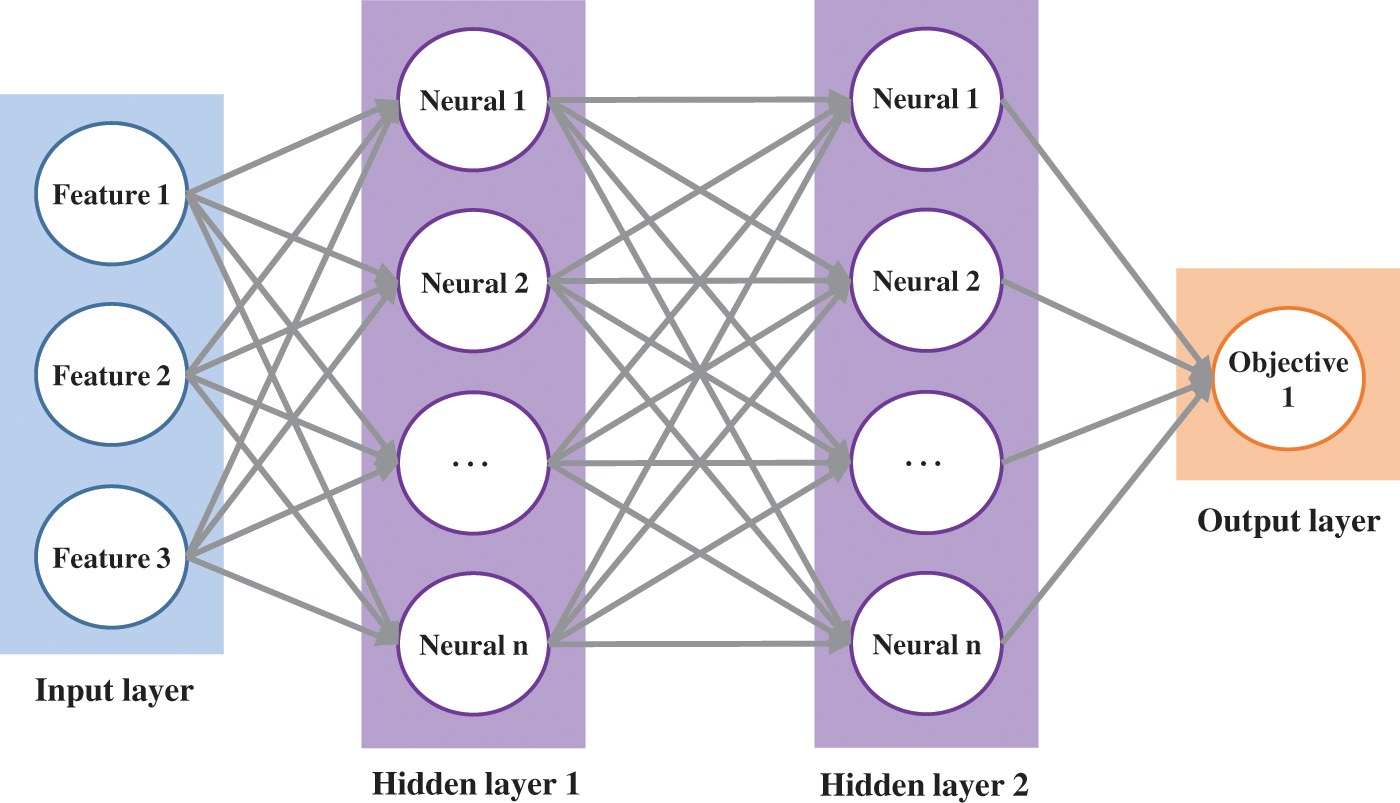
Figure 1: Diagram of a three-layer neural network
In theory, with a sufficient number of hidden layers and an adequate amount of training data, it is plausible to approximate any equation. The fundamental process of training a BPNN involves:
① Forward propagation from the input layer, where node outputs are computed, based on initialized parameters (random initialization) and activation functions, progressing until the output layer, subsequently calculating the error.
② Employing an optimizer to refine the error by utilizing backpropagation via the chain rule for derivative calculation, thereby updating weights and biases until meeting termination conditions.
2.4 Machine Learning Combination Model
Because various machine learning models operate on different principles, their efficacy in uncovering latent information within data also varies. These models are not mutually exclusive but rather complementary and can be interconnected. Relying solely on a single predictive model to determine hyperparameters for different datasets might introduce significant biases in prediction errors. Dismissing the use of the model could result in losing valuable insights it could have extracted, potentially leading to larger errors. Hence, ensemble models represent one effective approach to enhancing prediction accuracy. One critical issue in the machine learning combination model is how to construct it, and common methods for constructing the model include concatenated and parallel combination models.
(1) Concatenated combination model
This model involves utilizing the output of one model as the input for the next model. Each layer in the model can process and transform input data, extracting more useful features. The basic framework of the model is illustrated in Fig. 2.
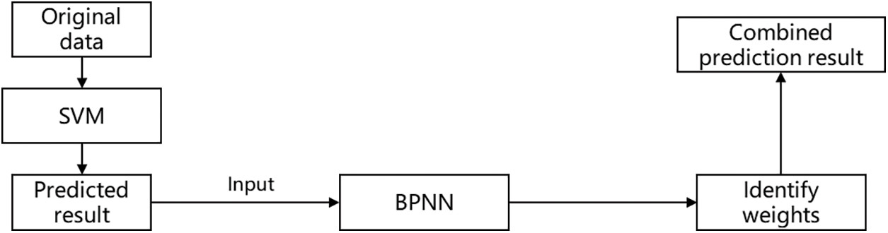
Figure 2: Diagram of concatenated combination model
(2) Parallel combination model
In this model, predictions from different models are combined through weighted averaging, where appropriate weights are assigned to each model’s prediction before merging. This approach yields more precise predictions, effectively handling generalization errors and overfitting. Simultaneously, it maintains higher accuracy and reliability. The basic framework of the model is illustrated in Fig. 3.
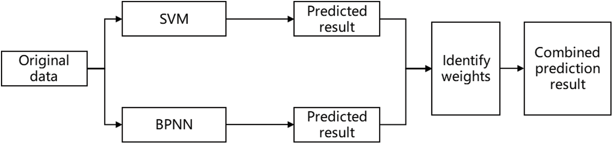
Figure 3: Diagram of parallel combination model
Compared to the concatenated combination model, the parallel combination model exhibits higher stability, operational efficiency, and stronger scalability. Consequently, for this study, a parallel combination model is chosen to establish the shale oil production capacity prediction model.
Furthermore, the final predictive performance of combination models closely correlates with weight determination. Different methods for calculating weights vary in difficulty and effectiveness. Common methods for weight determination include equal-weight averaging, error variance weighted averaging, and inverse relative error methods. To fully showcase the advantages of various machine learning algorithms in handling complex shale oil production capacity influencing factors, this study adopts the inverse relative error method to determine weight coefficients. The principle behind this method lies in utilizing relative errors to assess the predictive accuracy of models. Larger relative errors imply lower significance within the ensemble model, thus receiving lower weights. Conversely, smaller relative errors indicate better predictive performance, thereby obtaining higher weights within the ensemble predictive model. The formula for this method is:
where
3.1 Mathematical Model for the Flow in Shale Oil Reservoirs
When establishing a mathematical model for the three-phase flow of oil, gas, and water within shale oil reservoirs, several fundamental assumptions are typically made owing to the low density of shale oil, its tendency to contain dissolved gas, and the potential involvement of formation water in flow. These assumptions generally include: (1) The flow within the shale oil reservoir is isothermal; (2) Flow considerations for the oil and water phases account for threshold pressure gradients and stress sensitivity, while gas phase flow considers stress sensitivity only; (3) Hydrocarbons within the shale oil reservoir consist solely of oil and gas components, with the oil component exclusively present within the oil phase and the gas component able to exist in both the gas and oil phases; (4) Oil and gas are immiscible with water.
The permeability of shale oil reservoirs is extremely low, often in the nanodarcy range, showcasing distinct nonlinear characteristics in flow. The flow equation that incorporates threshold pressure gradients is given by:
where
Additionally, during the production of shale oil, the decline in reservoir pressure leads to an increase in effective stress on the rock, consequently causing a reduction in reservoir permeability. The relationship between shale permeability and effective stress can be expressed as:
where
where
Furthermore, to close the system of equations, the following auxiliary equations are required:
where
3.2 Data Analysis and Processing
This study included 225 wells from the R1 reservoir and 11 wells from the R2 reservoir. The field data associated with these wells is used to establish a data-driven approach for screening the main controlling factors affecting shale oil production capacity.
To precisely evaluate well performance and determine potential production, the analysis is conducted across two dimensions: Reservoir properties and well parameters. Reservoir properties such as porosity, oil saturation, permeability, density, and clay content are considered, directly impacting the storage and flow of hydrocarbons. Well parameters encompass specific configurations and operational details like the length of horizontal and oil layer segment length. With practical production cycles in mind, a three-month production period is selected as the benchmark for production capacity assessment, reflecting initial production conditions and providing ample data support.
A detailed data analysis, as shown in Table 1, reveals distinct differences between the R1 and R2 reservoirs across multiple parameters. Specifically, in terms of reservoir properties, R1’s reservoir density ranges from 2.38 to 2.61 g/cm³ with an average of 2.50 g/cm³, while R2’s is slightly higher, ranging from 2.52 to 2.66 g/cm³ with an average of 2.55 g/cm³. Additionally, variations are observed in clay content, permeability, porosity, and oil saturation between the two reservoirs. Overall, R1 slightly outperforms R2 in static reservoir evaluation parameters.
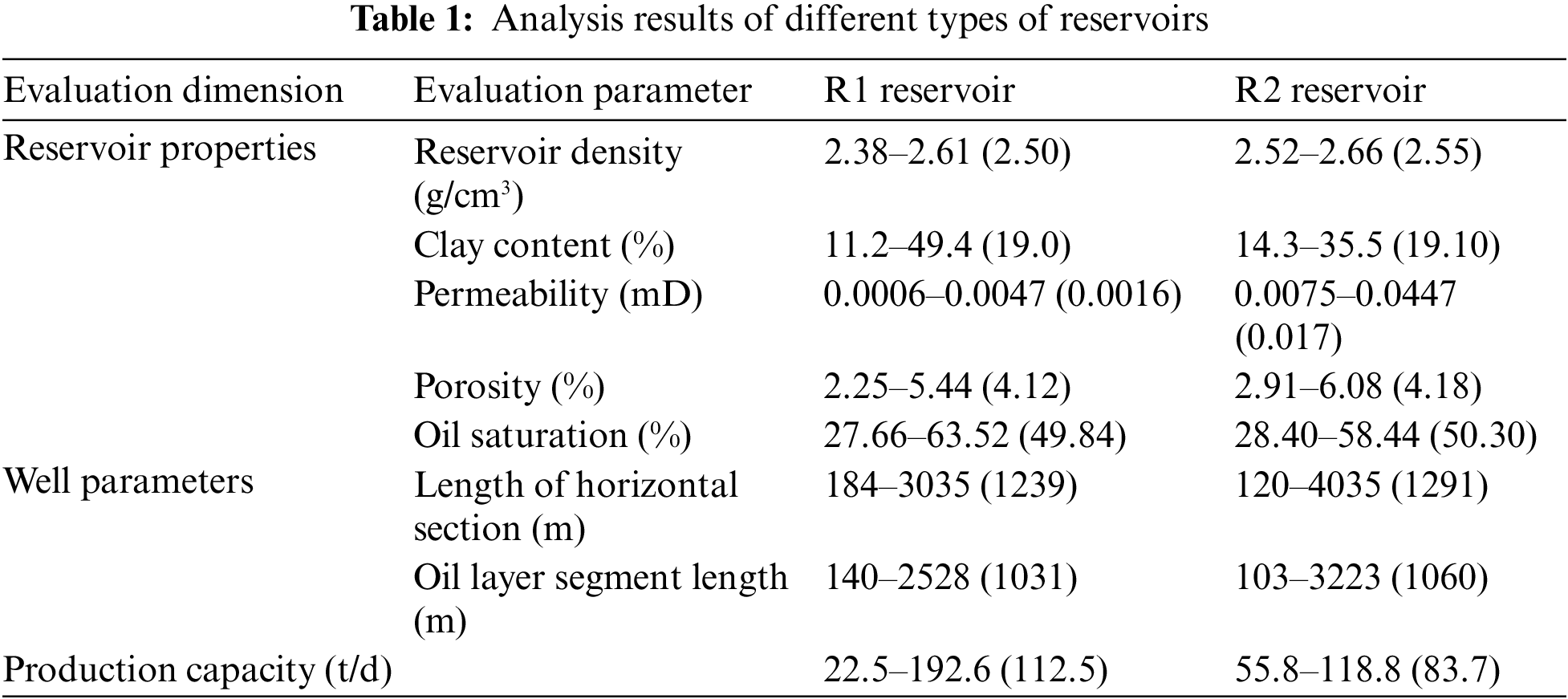
In well parameters, R1’s horizontal section length ranges from 184 to 3035 m, averaging 1239 m, compared to R2’s 120.0–4035.0 m, with an average of 1291 m. Differences in the oil layer segment length are also evident.
Crucially, in terms of production capacity, R1 ranges from 22.5 to 192.6 t/d, with an average of 112.5 t/d, significantly higher than R2’s 55.8 to 118.8 t/d, averaging 83.7 t/d. In summary, R1 exhibits a marginally superior performance across multiple evaluation dimensions, particularly in production capacity, providing essential data for further development of the shale oil field.
The factors influencing the horizontal well fracturing for shale oil can be broadly categorized into two types: A and B. Type A factors primarily consist of static parameters that determine the maximum potential production capacity in an ideal state. These include the size of the seepage area, the initial energy of the formation, and the formation’s seepage capability. In theory, type A represents the maximum potential production capacity under ideal conditions, assuming optimal reservoir working conditions without any non-physical interference.
Type B factors include dynamic and static parameters that reflect the depletion process of formation energy. They involve critical elements such as the elastic energy of the oil and the production rate. These core parameters reflect reservoir information and production dynamics, essential in the prediction process of early production capacity following shale oil horizontal well fracturing.
Given that type A encompasses numerous parameters, applying redundant parameters in production capacity prediction can degrade the predictive outcome. Therefore, it is crucial to select the main controlling factors from type A to ensure the accuracy of prediction results. In contrast, type B factors, reflecting essential reservoir and production dynamics, are indispensable in the early production capacity prediction process and do not require the same level of screening as type A.
Based on the field data of each well, this study uses an RF algorithm to screen the main controlling factors of the production capacity of different typical shale reservoirs. It can identify the factors that have the greatest impact on the shale oil production capacity under different geological, fluid, and well conditions and realize the data-driven main controlling factor screening. RF is an ensemble learning method mainly used for classification, regression, and feature selection, which has been widely adopted in petroleum engineering because of its robustness, accuracy, and ease of use.
Comprising numerous decision trees, each trained on a randomly selected subset of the data, RF finalizes its predictions through a voting or averaging process of all individual tree outcomes. This methodology excels at managing vast quantities of input variables and evaluating the significance of each, proving invaluable in multifactorial analyses where feature selection is crucial.
Based on the above methods, the main controlling factors affecting the fracturing development of different typical shale oil reservoirs are determined. In the R1 reservoir, the production capacity is predominantly governed by geological parameters, with the oil saturation, permeability, length of horizontal section, and reservoir density exerting a significant influence on production capacity. The detailed influence weights for the R1 reservoir are shown in Fig. 4.
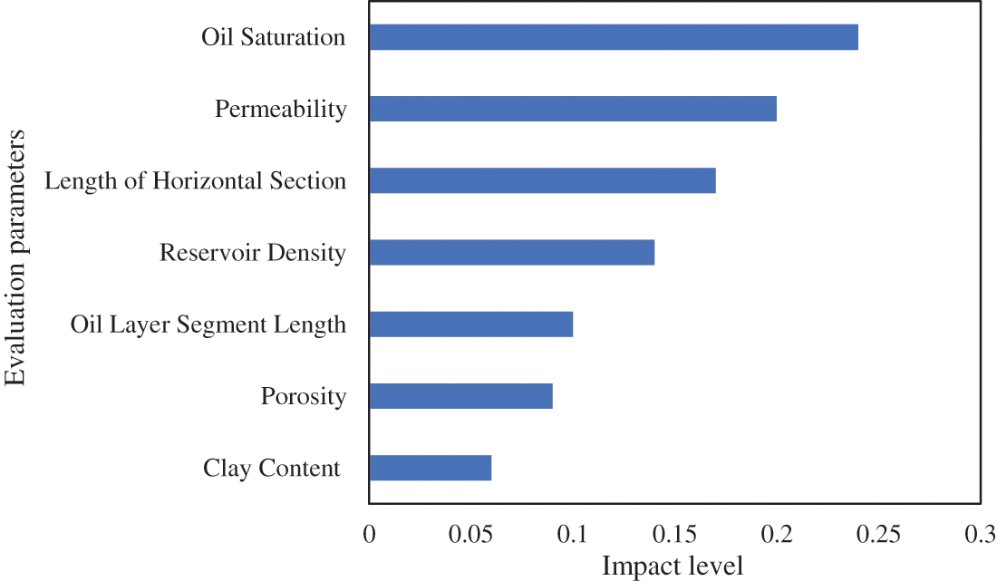
Figure 4: Influence weight of evaluation parameters for R1 reservoir
Conversely, the R2 reservoir exhibits inferior overall physical properties, leading to initial production capacity that is more substantially impacted by well parameters. Factors such as the oil layer segment length, length of horizontal section, permeability, and oil saturation are observed to have a considerable effect on production capacity levels. The detailed influence weights for the R2 reservoir are shown in Fig. 5.
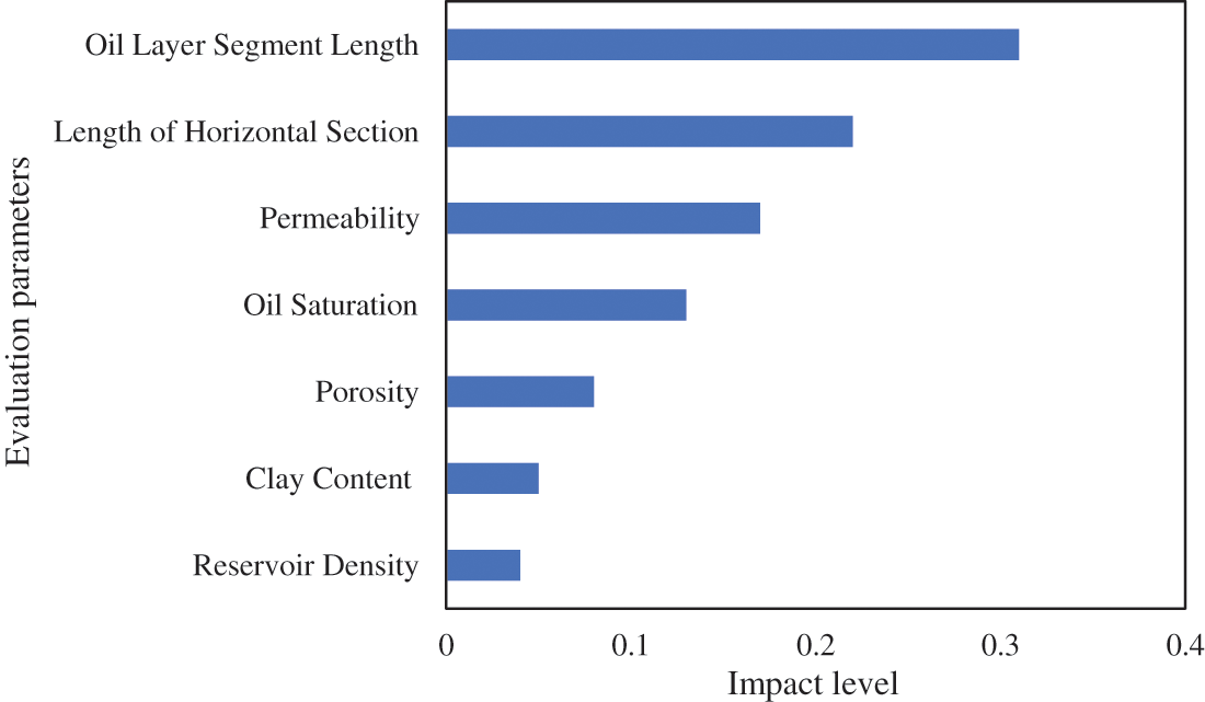
Figure 5: Influence weight of evaluation parameters for R2 reservoir
3.3 Construction of Production Capacity Prediction Sample Set
This study employs the reservoir numerical simulation method to construct a sample set for production capacity prediction, thereby establishing a model-driven approach for predicting shale oil production capacity. Focusing on the R1 and R2 reservoirs, a numerical simulation of horizontal well fracturing development considering threshold pressure gradients and stress sensitivity is carried out. Utilizing the E100 module of the Eclipse reservoir simulation software, a grid system for the foundational model is meticulously established. The model adheres to the Black Oil model, employing a block-centered grid within a Cartesian coordinate system. The grid system of the model comprises dimensions of 219 × 73 × 20, with grid steps of 20 m in both the X and Y directions, and a 1 m step in the Z direction.
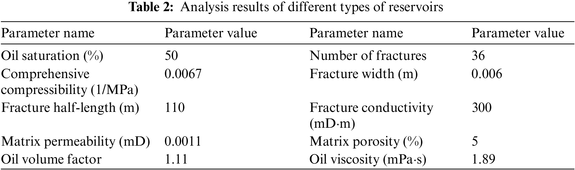
The specific attributes of the model include a vertical-to-horizontal permeability ratio of 0.1, with additional detailed parameters presented in Table 2. To precisely represent the petrophysical and fluid properties inherent in typical shale oil reservoirs, the initial temperature, pressure fields, and fluid phase states of the model have been calibrated to match the actual field data of the R1 and R2 reservoirs.
The 3D distribution of oil saturation for the shale oil reservoirs is depicted in Fig. 6, providing a visual representation of the reservoir characteristics. Through this comprehensive modeling and calibration process, the study ensures a high level of accuracy and reliability in the subsequent predictive analysis of production capacity in typical shale oil reservoirs.

Figure 6: Oil saturation model of the shale oil reservoir
Then, we encode an automated invocation program for the numerical simulator to build the production capacity prediction sample set efficiently. The framework of the program is shown in Fig. 7. The automated invocation program for numerical simulators utilizes Python to call the Eclipse environment within the computer, and batch processing of automatically generated typical shale oil DATA files is made possible. At the same time, multi-threaded processing of individual models significantly enhances operational efficiency. This ensures the automation of the entire process from the deployment of design parameters in numerical simulation, and parallel computing of multiple schemes, to the extraction and saving of simulation results, thereby forming a sample set for evaluating the production capacity of typical shale oil reservoirs and achieving a rapid and precise construction process for the database.
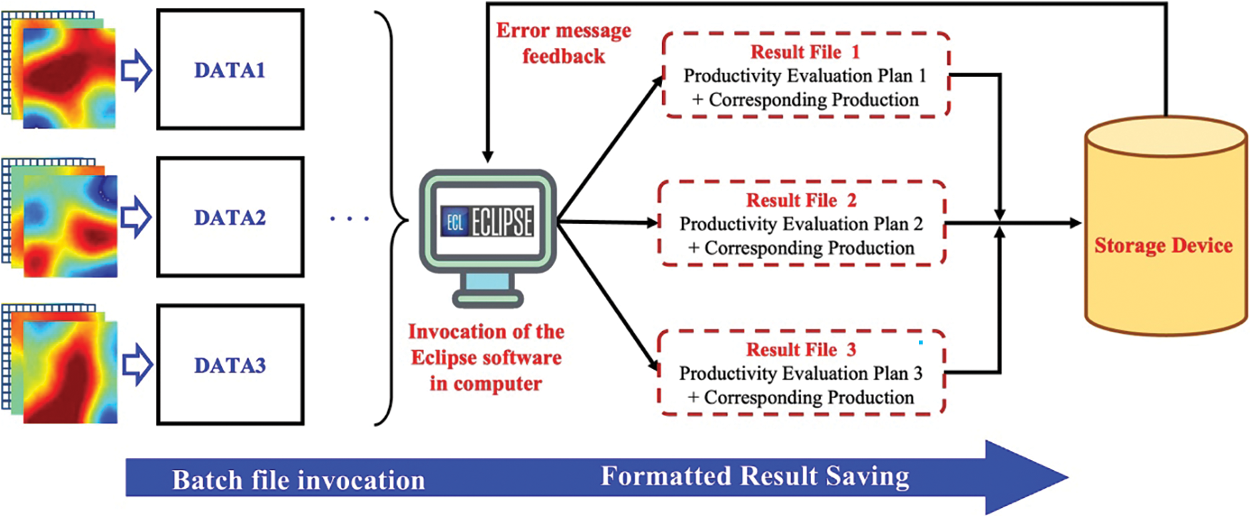
Figure 7: Flowchart of the automated invocation program for numerical simulators
In this study, the automated invocation program for numerical simulators is used to simulate the production dynamics of R1 and R2 reservoirs for 800 and 300 times, respectively. Subsequently, data normalization procedures are applied to ensure the compatibility of the production capacity sample set of typical shale oil reservoirs with various prediction models, including the SVM algorithm, BPNN, and their combination model.
Due to the disparate dimensions and significant magnitude differences among the aforementioned input parameters, the complexity of model construction is increased, potentially leading to a decrease in accuracy. To circumvent numerical and dimensional issues arising from variations between different parameters, data preprocessing is commonly employed. In this study, the Z-Score normalization method is utilized to process the input parameters. Models built with standardized data exhibit faster execution speeds and yield superior predictive performance. The formula for the Z-Score normalization is given below:
where
After completing the above operations, the production capacity prediction sample set has been established and can be used in the training process of the model.
3.4 Shale Oil Productivity Prediction Modelling
This study aims to establish a production capacity prediction model using machine learning methods in typical shale oil reservoirs. The model employs the main controlling factors affecting production capacity undergoing hydraulic fracturing as input data. The average daily oil production three months post-production serves as the output data. The objective is to enable a comprehensive, multifactorial prediction of shale oil production capacity under various geological, fluid, and hydraulic fracturing development conditions, facilitating a swift response to the potential of shale oil hydraulic fracturing development.
According to the screening results of the main controlling factors, it is determined that This study aims to establish a production capacity prediction model using machine learning methods in typical shale oil reservoirs. The model employs the main controlling factors affecting production capacity undergoing hydraulic fracturing as input data. The average daily oil production three months post-production serves as the output data. The objective is to enable a comprehensive, multifactorial prediction of shale oil production capacity under various geological, fluid, and hydraulic fracturing development conditions, facilitating a swift response to the potential of shale oil hydraulic fracturing development.
According to the screening results of the main controlling factors, it is determined that oil saturation, permeability, length of the horizontal section, and reservoir density are the main controlling factors affecting the production capacity of the R1 reservoir. The oil layer segment length, length of the horizontal section, permeability, and oil saturation are the main factors affecting the production capacity of the R2 reservoir. These main controlling factors serve as the input parameters for type A in the R1 reservoir and R2 reservoir production capacity prediction model, employed for predicting the production capacity of typical shale oil. Meanwhile, type B encompasses production rate, reservoir pressure, and the gas-oil ratio of dissolved gas, adding three more factors to be incorporated into the prediction model. Consequently, the input parameters for the R1 reservoir and R2 reservoir production capacity prediction model contain seven factors respectively. These factors together with the outputs (shale oil production capacity) constitute the shale oil production capacity prediction sample set.
To conduct a training process on the production capacity prediction sample set for the shale oil reservoir, it is necessary to partition the samples. They are divided into training, testing, and validation sets in certain proportions, serving the purposes of training the shale oil production capacity prediction model, optimizing various machine learning algorithm hyperparameters, and verifying the model’s training outcomes. In this study, 800 numerical simulation runs are generated for the R1 reservoir by randomly matching different geological, fluid, and hydraulic fracturing development parameters. Specifically, 640 models (80% of the sample set) are utilized to train the shale oil production capacity prediction model based on the loss function, 80 models (10% of the sample set) are used to adjust different machine learning algorithm hyperparameters, and the final 80 models (10% of the sample set) are employed to validate the predictive performance of the model. Additionally, to showcase the impact of sample size on various machine learning methods, 300 numerical simulation runs are created for the R2 reservoir. These are split into 240 models for training, 30 for testing, and 30 for validation purposes.
In tackling the regression problem with multiple input parameters, this study employs two distinct mainstream machine learning methods and their combination to construct prediction models: SVM and BPNN. Given that the objective of this study is to establish a shale oil production capacity prediction model applicable to scenarios with varying sizes of field data, it is noteworthy that BPNN, known for its capability in handling high-dimensional and large-scale datasets, can capture complex nonlinear relationships. SVM, on the other hand, demonstrates clear superiority in handling small sample datasets compared to other ML methods. Therefore, for the shale oil production capacity prediction problem addressed in this study, a parallel combination model integrating SVM and BPNN is chosen to leverage their respective strengths.
The primary step involves determining the pertinent parameters of these diverse machine-learning methods to suit the sample set. These encompass standard parameters (like weights and biases) and hyperparameters (such as neural network layers). Standard parameters are typically resolved through routine learning and training, while hyperparameters are usually optimized using manual or grid search methods to compare the performance of network models on the validation set under various parameter combinations, thereby facilitating optimal selection. However, these conventional methods often encounter difficulties such as slow convergence and susceptibility to local optima. The Particle Swarm Optimization (PSO) algorithm exhibits robust self-organizing learning capabilities, strong global search prowess, swift convergence, and ease of parameter implementation. Consequently, in constructing a prediction model, the PSO algorithm is employed to optimize the hyperparameters of SVM and BPNN.
Furthermore, to assess the accuracy of the selected machine learning methods in predicting production capacity and their model generalization, this study employs the determination coefficient (R²), mean squared error (MSE), and mean absolute error (MAE) to evaluate the predictive performance of the shale oil production capacity model. The calculation process for each is depicted respectively in Eqs. (20) to (22):
where
Forecasting production capacity is crucial for assessing new well productivity and evaluating economic returns. Establishing a shale oil production capacity prediction model based on geological, fluid, and hydraulic fracturing development parameters enables approximating well productivity using production decline patterns. This approach aids in promptly adjusting development strategies and production strategies for wells, optimizing their performance and operational efficacy.
Based on the geological and engineering factors that influence production capacity, this study employs the SVM algorithm, BPNN, and their combination model to predict the production capacity of typical shale oil reservoirs. The R2, MSE, and MAE are used to evaluate the performance of different models. By parallelly connecting the SVM algorithm and BPNN, a combination prediction model is constructed. The performance of individual prediction models and the combination prediction model in different typical shale oil reservoirs is then compared and analyzed.
Firstly, a shale oil production capacity prediction model based on the SVM algorithm is established, followed by hyperparameter optimization using the testing set. A crucial aspect of SVM regression is the selection of the kernel function type, which includes linear, polynomial, sigmoid, and Gaussian RBF kernel functions. Among these, the RBF kernel function is widely applied. While selecting a linear kernel can mitigate extensive computational requirements when the sample set features high-dimensional characteristics and a sufficient quantity of samples, the RBF kernel function consistently demonstrates excellent performance, irrespective of sample size or data dimensionality. Additionally, another critical hyperparameter in SVM is the penalty factor C, which determines the degree of loss for outliers. Smaller C values correspond to smaller losses in the objective function. In this study, the SVM hyperparameters resulting from PSO optimization are determined as RBF kernel functions with C = 3. Following modeling, the SVM-based shale oil production capacity prediction model is validated on the R1 and R2 reservoirs. Comparisons between predicted and actual results on the training and validation sets are depicted in Figs. 8 and 9, demonstrating R2 values of 0.74 and 0.82, respectively.
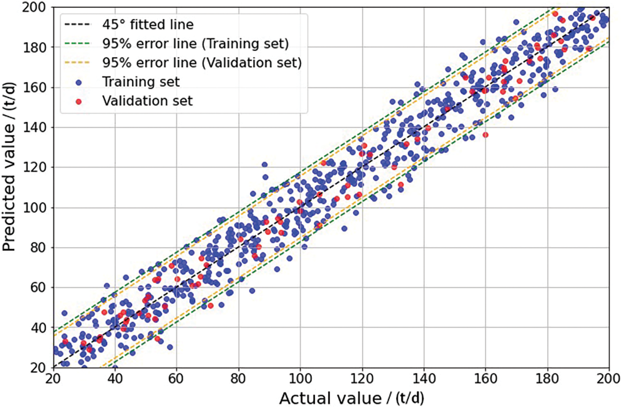
Figure 8: Comparison of SVM-based predictions with actual results in R1
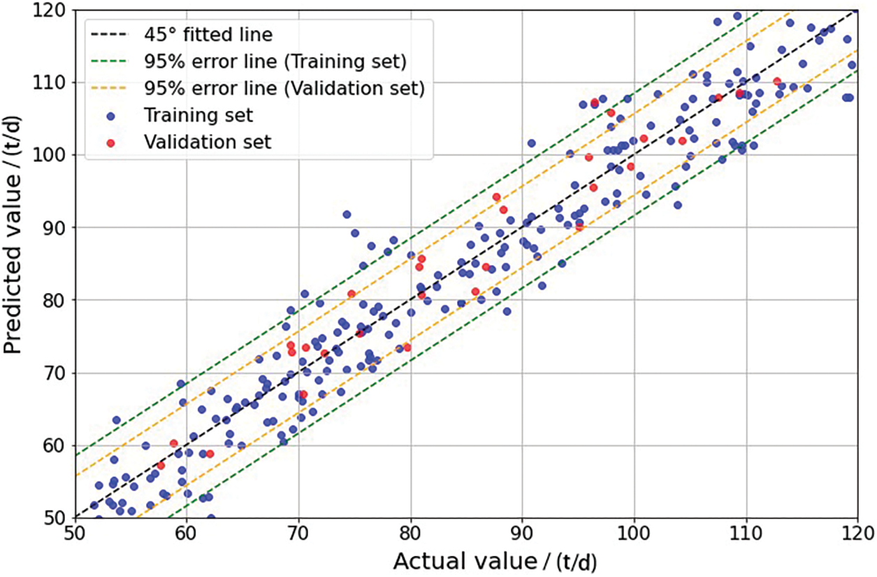
Figure 9: Comparison of SVM-based predictions with actual results in R2
The inclusion of a regularization term in SVM helps mitigate overfitting caused by substantial randomness in shale oil development data, as well as complex main controlling factors affecting production, contributing to the model’s robust generalization ability. Particularly, when dealing with numerous well parameters with weak interdependencies, SVM demonstrates good predictive performance without further feature selection, especially in scenarios with high-dimensional features and limited sample size. In this study, compared to the R1 reservoir, SVM exhibits better performance when applied to the R2 reservoir. This is attributed to SVM’s superior performance in handling small sample datasets, allowing for smooth training on the 240 samples (training set for R2 reservoir) available in this dataset. Consequently, SVM becomes suitable for production capacity prediction in situations involving a multitude of features and poor parameter independence.
Subsequently, a shale oil production capacity prediction model is developed based on the BPNN, employing a testing set to determine the network’s hyperparameters such as the number of hidden layers and neurons, further optimized using the PSO algorithm. The optimal hyperparameter combination yielded a model with three hidden layers and ten neurons. To map features into higher dimensions for fitting nonlinear functions, the model employs the ReLU activation function during weight propagation from input to hidden layers, facilitating the model’s ability to capture nonlinear patterns. Following model construction, the BPNN-based shale oil production capacity prediction model is validated on the R1 and R2 reservoirs. Comparisons between predicted and actual results on the training and validation sets are presented in Figs. 10 and 11, indicating R2 values of 0.86 and 0.77, respectively.
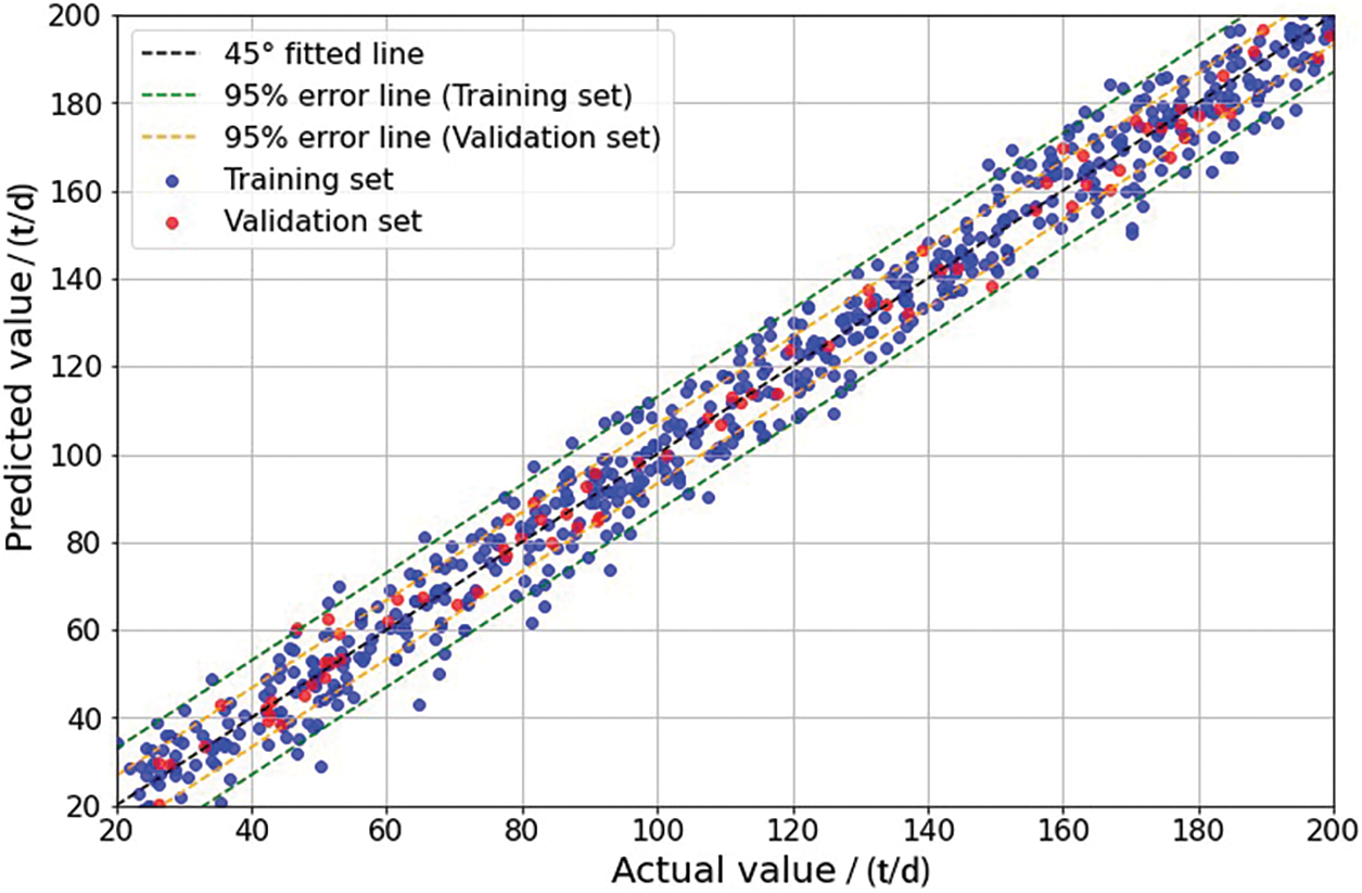
Figure 10: Comparison of BPNN-based predictions with actual results in R1
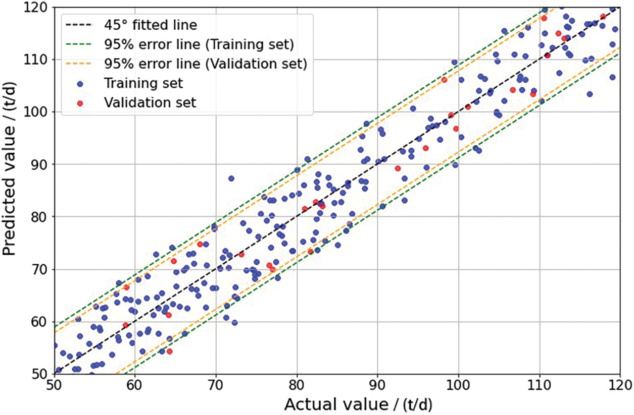
Figure 11: Comparison of BPNN-based predictions with actual results in R2
On the R1 reservoir, the abundance of data used for training the BPNN allows for a robust fitting of nonlinear relationships between factors and production, resulting in higher prediction accuracy compared to the SVM algorithm. This makes it more suitable for production capacity prediction in this oil field. Essentially, the BPNN inherently fits features to prediction targets, providing superior descriptions of their nonlinear relationships compared to non-neural network models. Consequently, it performs better in production capacity prediction scenarios characterized by complex factor-production relationships. However, on the R2 reservoir, where the dataset contains fewer samples. The SVM algorithm is adept at handling multi-feature, small-sample data and outperforms due to the inability to sufficiently train the BPNN. Therefore, it can be observed that in shale oil production capacity prediction, SVM excels in handling on-site data with a scarcity of samples, especially in the presence of numerous missing or outlier values, while achieving the desired predictive outcomes. On the other hand, BPNN is more suitable for shale oil production capacity prediction when an ample amount of data is available, demonstrating superior predictive performance compared to traditional ML methods. Consequently, in addressing predictive problems involving the various data volumes of multiple shale oil reservoirs, it is necessary to leverage the strengths and weaknesses of both algorithms to handle the complexities of varying data volumes effectively.
Finally, integrating SVM and BPNN as base learners forms a machine-learning combination model. The hyperparameter settings for the combination model align with the optimization results mentioned earlier. In this study, a weighted averaging method is employed to integrate different base learners into the combination model, as depicted in Eq. (23):
where
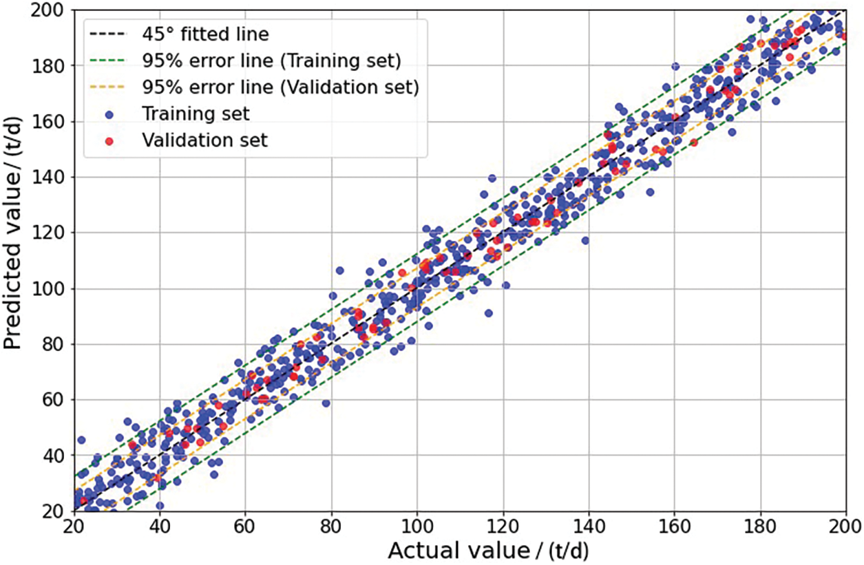
Figure 12: Comparison of combination model-based predictions with actual results in R1
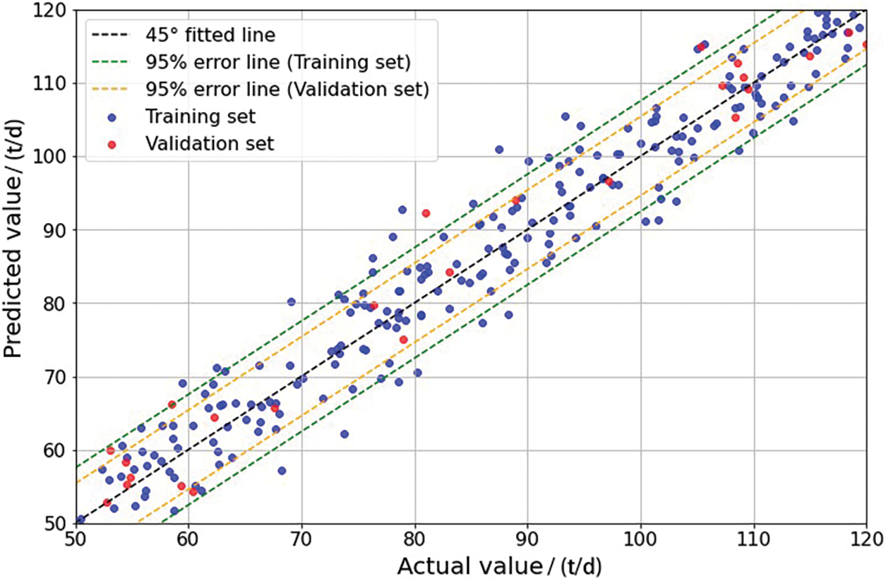
Figure 13: Comparison of combination model-based predictions with actual results in R2
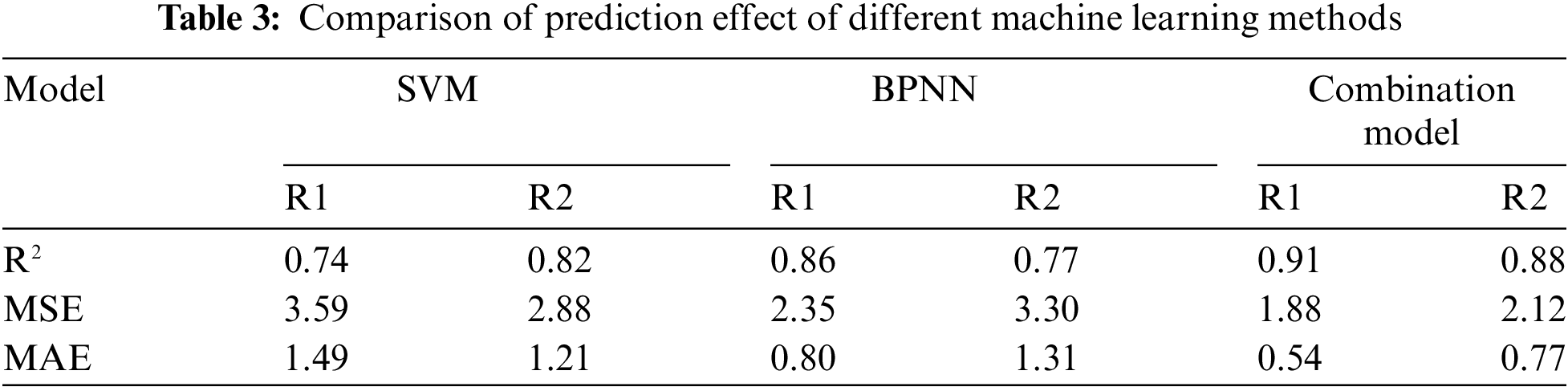
Additionally, the performance of different models on the production capacity prediction sample set is detailed in Table 3. The combination model noticeably improves predictive accuracy while reducing MSE and MAE compared to individual models. This indicates that by harnessing the advantages of various base learners in handling shale oil production capacity data, the combination model demonstrates superior predictive performance. SVM performs well, especially in scenarios with limited dataset samples and numerous input features such as R2 reservoirs. Conversely, BPNN excels in uncovering nonlinear relationships among diverse influencing factors, leading to more precise fitting when dataset samples are ample, just like R1 reservoirs. These aspects could underlie the enhanced performance of the combination model in shale oil production capacity prediction. The shale oil production capacity prediction model established based on the combination model shows that when dealing with small sample datasets, the SVM part of the combination model plays a more significant role, carrying greater weight and yielding superior predictive performance. Conversely, when handling large-scale datasets, the BPNN part carries more weight and exerts greater influence on the predictive outcomes, leading to more precise predictions. Consequently, by alternating the weights between SVM and BPNN depending on the dataset volume, optimal predictive performance can be achieved across varying sample sizes. Integrating the strengths of both machine learning methods, the combination model exhibits superior predictive efficacy, capturing the fundamental dynamics of post-fracturing shale oil production. Hence, the combination model offers heightened reliability and practicality in predicting shale oil production dynamics, establishing its utility in this domain.
This paper addresses the challenge of swiftly and accurately assessing the effects of hydraulic fracturing development in shale oil wells. By leveraging the advantages of both data-driven and model-driven methodologies, a combined machine learning model for predicting shale oil productivity is established. Utilizing hydraulic fracturing development data from 236 wells, a data-driven method based on the Random Forest algorithm is used to identify the main controlling factors for different types of shale oil reservoirs. Furthermore, a model-driven prediction model for shale oil productivity is developed by integrating Support Vector Machine algorithms and Back Propagation Neural Network. This model can rapidly respond to the dynamic development performance of shale oil under geological and engineering uncertainties.
1. The data-driven method based on a random forest algorithm is utilized to screen the main controlling factor for shale oil reservoir production capacity. It distinctly identifies that the production capacity is primarily influenced by geological parameters such as oil saturation, permeability, length of horizontal section, and reservoir density within the R1 reservoir. The production capacity is predominantly influenced by well parameters just as oil layer segment length, length of horizontal section, permeability, and oil saturation in the R2 reservoir.
2. The combination model, incorporating SVM and BPNN base learners, establishes a model-driven prediction model for shale oil production capacity. This model enables a swift response toward shale oil production capacity under diverse geological, fluid, and hydraulic fracturing development conditions.
3. The combination model demonstrates superior performance across various datasets compared to singular machine learning methods like SVM and BPNN. SVM performs well when handling limited dataset samples with numerous input features just as the R2 reservoir. Conversely, BPNN excels in revealing nonlinear relationships among various influencing factors when ample dataset samples are available, as demonstrated in the R1 reservoir. Integrating the strengths of base learners, the combination model consistently outperforms in handling diverse datasets. It confirms that the combination model offers heightened reliability and practicality in predicting shale oil production dynamics, establishing its utility in the petroleum engineering domain.
4. The method proposed in this paper demonstrates good performance in handling datasets with varying sample sizes, effectively addressing the prediction challenges arising from differences in data volume among different wells in oilfield sites. However, the method also exhibits limitations. As the sub-learners utilized are based on fundamental machine learning techniques, they are unable to account for complex high-dimensional data containing additional reservoir information, such as permeability fields, saturation fields, and temporal variations in production data. Future research will focus on addressing these shortcomings by integrating methods like deep learning and reinforcement learning to develop production capacity prediction approaches suitable for a broader range of reservoir development scenarios.
Acknowledgement: None.
Funding Statement: This work was supported by the China Postdoctoral Science Foundation (2021M702304) and Natural Science Foundation of Shandong Province (ZR20210E260).
Author Contributions: The authors confirm contribution to the paper as follows: Study conception and design: Qin Qian, Yuliang Su; data collection: Mingjing Lu; analysis and interpretation of results: Anhai Zhong, Wenjun He; draft manuscript preparation: Feng Yang, Min Li. All authors reviewed the results and approved the final version of the manuscript.
Availability of Data and Materials: The data that has been used is confidential.
Conflicts of Interest: The authors declare that they have no conflicts of interest to report regarding the present study.
References
1. W. Wang, W. Yu, S. Wang, L. Zhang, Q. Zhang and Y. Su, “Mitigating interwell fracturing interference: Numerical investigation of parent well depletion affecting infill well stimulation,” J. Energy Resour. Technol., vol. 146, no. 1, pp. 013502, Jan. 2024. doi: 10.1115/1.4063490. [Google Scholar] [CrossRef]
2. Y. Liu, J. Zeng, J. Qiao, G. Yang, and W. Cao, “An advanced prediction model of shale oil production profile based on source-reservoir assemblages and artificial neural networks,” Appl. Energy, vol. 333, pp. 120604, Mar. 2023. doi: 10.1016/j.apenergy.2022.120604. [Google Scholar] [CrossRef]
3. W. Wang et al., “Pore-scale simulation of multiphase flow and reactive transport processes involved in geologic carbon sequestration,” Earth-Sci. Rev., vol. 247, pp. 104602, Dec. 2023. doi: 10.1016/j.earscirev.2023.104602. [Google Scholar] [CrossRef]
4. W. Wang et al., “Current status and development trends of CO2 storage with enhanced natural gas recovery (CS-EGR),” Fuel, vol. 349, pp. 128555, Oct. 2023. doi: 10.1016/j.fuel.2023.128555. [Google Scholar] [CrossRef]
5. J. Schuetter, S. Mishra, M. Zhong, and R. LaFollette, “A data-analytics tutorial: Building predictive models for oil production in an unconventional shale reservoir,” SPE J., vol. 23, no. 4, pp. 1075–1089, Mar. 2018. doi: 10.2118/189969-PA. [Google Scholar] [CrossRef]
6. W. Wang, Q. Xie, H. Wang, Y. Su, and S. R. Gomari, “Pseudopotential-based multiple-relaxation-time lattice boltzmann model for multicomponent and multiphase slip flow,” Adv. Geo-Energ. Res., vol. 9, no. 2, pp. 106–116, Mar. 2023. doi: 10.46690/ager.2023.08.04. [Google Scholar] [CrossRef]
7. P. Panja, R. Velasco, M. Pathak, and M. Deo, “Application of artificial intelligence to forecast hydrocarbon production from shales,” Petroleum, vol. 4, no. 1, pp. 75–89, Mar. 2018. doi: 10.1016/j.petlm.2017.11.003. [Google Scholar] [CrossRef]
8. W. Niu, J. Lu, and Y. Sun, “An improved empirical model for rapid and accurate production prediction of shale gas wells,” J. Pet. Sci. Eng., vol. 208, pp. 109800, Jan. 2022. doi: 10.1016/j.petrol.2021.109800. [Google Scholar] [CrossRef]
9. Q. Xie, W. Wang, Y. Su, H. Wang, Z. Zhang and W. Yan, “Pore-scale study of calcite dissolution during CO2-saturated brine injection for sequestration in carbonate aquifers,” Gas Sci. Eng., vol. 114, pp. 204978, Jun. 2023. doi: 10.1016/j.jgsce.2023.204978. [Google Scholar] [CrossRef]
10. F. Male, “Using a segregated flow model to forecast production of oil, gas, and water in shale oil plays,” J. Pet. Sci. Eng., vol. 180, pp. 48–61, Sep. 2019. doi: 10.1016/j.petrol.2019.05.010. [Google Scholar] [CrossRef]
11. V. Nguyen-Le, H. Shin, and E. Little, “Development of shale gas prediction models for long-term production and economics based on early production data in Barnett reservoir,” Energies, vol. 13, no. 2, pp. 424, Jan. 2020. doi: 10.3390/en13020424. [Google Scholar] [CrossRef]
12. W. Niu, J. Lu, and Y. Sun, “A production prediction method for shale gas wells based on multiple regression,” Energies, vol. 14, no. 5, pp. 1461, Mar. 2021. doi: 10.3390/en14051461. [Google Scholar] [CrossRef]
13. G. Zhou, Z. Guo, S. Sun, and Q. Jin, “A CNN-BiGRU-AM neural network for AI applications in shale oil production prediction,” Appl. Energy, vol. 344, pp. 121249, Aug. 2023. doi: 10.1016/j.apenergy. [Google Scholar] [CrossRef]
14. K. Lee, J. Lim, D. Yoon, and H. Jung, “Prediction of shale-gas production at duvernay formation using deep-learning algorithm,” SPE J., vol. 24, no. 62, pp. 2423–2437, Jul. 2019. doi: 10.2118/195698-PA. [Google Scholar] [CrossRef]
15. Q. Wang and F. Jiang, “Integrating linear and nonlinear forecasting techniques based on grey theory and artificial intelligence to forecast shale gas monthly production in Pennsylvania and Texas of the United States,” Energy, vol. 178, pp. 781–803, Jul. 2019. doi: 10.1016/j.energy.2019.04.115. [Google Scholar] [CrossRef]
16. Y. Zhang, D. Lv, Y. Wang, H. Liu, G. Song and J. Gao, “Geological characteristics and abnormal pore pressure prediction in shale oil formations of the Dongying depression,” China Energ. Sci. Eng., vol. 8, no. 6, pp. 1962–1979, Feb. 2020. doi: 10.1002/ese3.641. [Google Scholar] [CrossRef]
17. F. I. Syed, S. Alnaqbi, T. Muther, A. K. Dahaghi, and S. Negahban, “Smart shale gas production performance analysis using machine learning applications,” Petroleum Res., vol. 7, no. 1, pp. 21–31, Mar. 2022. doi: 10.1016/j.ptlrs.2021.06.003. [Google Scholar] [CrossRef]
18. Y. Su et al., “Spontaneous imbibition characteristics of shale oil reservoir under the influence of osmosis,” Int. J. Coal Sci.Techn., vol. 9, no. 1, pp. 69, Sep. 2022. doi: 10.1007/s40789-022-00546-5. [Google Scholar] [CrossRef]
19. M. Zoveidavianpoor and A. Gharibi, “Applications of type-2 fuzzy logic system: Handling the uncertainty associated with candidate-well selection for hydraulic fracturing,” Neural Comput. Appl., vol. 27, pp. 1831–1851, Jul. 2015. doi: 10.1007/s00521-015-1977-x. [Google Scholar] [CrossRef]
20. A. Davarpanah, R. Shirmohammadi, B. Mirshekari, and A. Aslani, “Analysis of hydraulic fracturing techniques: Hybrid fuzzy approaches,” Arab. J. Geosci., vol. 12, pp. 1–8, Jun. 2019. doi: 10.1007/s12517-019-4567-x. [Google Scholar] [CrossRef]
21. B. Gou, C. Wang, T. Yu, and K. Wang, “Fuzzy logic and grey clustering analysis hybrid intelligence model applied to candidate-well selection for hydraulic fracturing in hydrocarbon reservoir,” Arab. J. Geosci., vol. 13, pp. 1–13, Sep. 2020. doi: 10.1007/s12517-020-05970-y. [Google Scholar] [CrossRef]
22. V. Nguyen-Le, H. Shin, and Z. Chen, “Deep neural network model for estimating montney shale gas production using reservoir, geomechanics, and hydraulic fracture treatment parameters,” Gas Sci. Eng., vol. 120, pp. 205161, Dec. 2023. doi: 10.1016/j.jgsce.2023.205161. [Google Scholar] [CrossRef]
23. H. Klie and H. Florez, “Data-driven prediction of unconventional shale-reservoir dynamics,” SPE J., vol. 25, no. 5, pp. 2564–2581, Sep. 2022. doi: 10.2118/193904-PA. [Google Scholar] [CrossRef]
24. D. A. Otchere, T. O. A. Ganat, R. Gholami, and S. Ridha, “Application of supervised machine learning paradigms in the prediction of petroleum reservoir properties: Comparative analysis of ANN and SVM models,” J. Pet. Sci. Eng., vol. 200, pp. 108182, May 2021. doi: 10.1016/j.petrol.2020.108182. [Google Scholar] [CrossRef]
25. H. Alimohammadi and S. N. Chen, “Long-term production forecast in tight and shale reservoirs: Adapting probability density functions for decline curve analysis,” Gas Sci. Eng., vol. 118, pp. 205113, Oct. 2023. doi: 10.1016/j.jgsce.2023.205113. [Google Scholar] [CrossRef]
26. W. G. Davies, S. Babamohammadi, Y. Yang, and S. M. Soltani, “The rise of the machines: A state-of-the-art technical review on process modelling and machine learning within hydrogen production with carbon capture,” Gas Sci. Eng., vol. 118, pp. 205104, Oct. 2023. doi: 10.1016/j.jgsce.2023.205104. [Google Scholar] [CrossRef]
27. Q. Zhou, A. Kleit, J. Wang, and R. Dilmore, “Evaluating gas production performances in marcellus using data mining technologies,” in Unconventional Resources Technology Conf., Denver, Colorado, USA, Aug. 25–27, 2014. [Google Scholar]
28. E. Lolon, K. Hamidieh, L. Weijers, M. Mayerhofer, H. Melcher and O. Oduba, “Evaluating the relationship between well parameters and production using multivariate statistical models: A middle bakken and three forks case history,” in SPE Hydraul. Fracturing Technol. Conf. Exhibition, Woodlands, Texas, USA, Feb. 9–11, 2016. [Google Scholar]
29. S. D. Mohaghegh, R. Gaskari, and M. Maysami, “Shale analytics: Making production and operational decisions based on facts: A case study in marcellus shale,” in SPE Hydraul. Fracturing Technol. Conf. Exhibition, Woodlands, Texas, USA, Jan. 24–26, 2017. [Google Scholar]
30. C. Lu, H. Jiang, J. Yang, Z. Wang, M. Zhang and J. Li, “Shale oil production prediction and fracturing optimization based on machine learning,” J. Pet. Sci. Eng., vol. 217, pp. 110900, Oct. 2022. doi: 10.1016/j.petrol.2022.110900. [Google Scholar] [CrossRef]
31. P. Mahzari, M. Emambakhsh, C. Temizel, and P. A. Jones, “Oil production forecasting using deep learning for shale oil wells under variable gas-oil and water-oil ratios,” Pet. Sci. Technol., vol. 40, no. 4, pp. 445–468, Nov. 2021. doi: 10.1080/10916466.2021.2001526. [Google Scholar] [CrossRef]
32. G. Hui, Z. Chen, Y. Wang, D. Zhang, and F. Gu, “An integrated machine learning-based approach to identifying controlling factors of unconventional shale productivity,” Energy, vol. 266, pp. 126512, Mar. 2023. doi: 10.1016/j.energy.2022.126512. [Google Scholar] [CrossRef]
33. C. Wu, S. Wang, J. Yuan, C. Li, and Q. Zhang, “A prediction model of specific productivity index using least square support vector machine method,” Adv. Geo-Ener. Res., vol. 4, no. 4, pp. 460–467, Dec. 2020. doi: 10.46690/ager.2020.04.10. [Google Scholar] [CrossRef]
34. X. Y. Zhuang et al., “Multi-objective optimization of water-flooding strategy with hybrid artificial intelligence method,” Expert Syst. Appl., vol. 241, pp. 122707, May 2024. doi: 10.1016/j.eswa.2023.122707. [Google Scholar] [CrossRef]
35. Q. Wang et al., “A novel method for petroleum and natural gas resource potential evaluation and prediction by support vector machines (SVM),” Appl. Energy, vol. 351, pp. 121836, Dec. 2023. doi: 10.1016/j.apenergy.2023.121836. [Google Scholar] [CrossRef]
36. H. Luo, F. Q. Lai, Z. Dong, and W. X. Xia, “A lithology identification method for continental shale oil reservoir based on BP neural network,” J. Geophys. Eng., vol. 15, no. 3, pp. 895–908, Jun. 2018. doi: 10.1088/1742-2140/aaa4db. [Google Scholar] [CrossRef]
Cite This Article
 Copyright © 2024 The Author(s). Published by Tech Science Press.
This work is licensed under a Creative Commons Attribution 4.0 International License , which permits unrestricted use, distribution, and reproduction in any medium, provided the original work is properly cited.
 Downloads
 Citation Tools