
 Submit a Paper
 Propose a Special lssue
 Open Access
ARTICLE

A Disturbance Localization Method for Power System Based on Group Sparse Representation and Entropy Weight Method
1 Changchun Power Supply Company, State Grid Jilin Electric Power Co., Ltd., Changchun, 130021, China
2 Economic and Technical Research Institute, State Grid Jilin Electric Power Co., Ltd., Changchun, 130022, China
3 Key Laboratory of Modern Power System Simulation and Control & Renewable Energy Technology, Northeast Electric Power University, Jilin, 132012, China
* Corresponding Author: Shiqiang Li. Email:
Energy Engineering 2024, 121(8), 2275-2291. https://doi.org/10.32604/ee.2024.028223
Received 06 December 2022; Accepted 24 February 2023; Issue published 19 July 2024
 View Full Text
 Download PDF
Abstract
This paper addresses the problem of complex and challenging disturbance localization in the current power system operation environment by proposing a disturbance localization method for power systems based on group sparse representation and entropy weight method. Three different electrical quantities are selected as observations in the compressed sensing algorithm. The entropy weighting method is employed to calculate the weights of different observations based on their relative disturbance levels. Subsequently, by leveraging the topological information of the power system and pre-designing an overcomplete dictionary of disturbances based on the corresponding system parameter variations caused by disturbances, an improved Joint Generalized Orthogonal Matching Pursuit (J-GOMP) algorithm is utilized for reconstruction. The reconstructed sparse vectors are divided into three parts. If at least two parts have consistent node identifiers, the node is identified as the disturbance node. If the node identifiers in all three parts are inconsistent, further analysis is conducted considering the weights to determine the disturbance node. Simulation results based on the IEEE 39-bus system model demonstrate that the proposed method, utilizing electrical quantity information from only 8 measurement points, effectively locates disturbance positions and is applicable to various disturbance types with strong noise resistance.Keywords
Nomenclature
| PMU | Phase measurement units |
| OMP | Orthogonal matching pursuit |
| GOMP | Generalized orthogonal matching pursuit |
| IST | Iterative Shrink-age-Thresholding |
| ALM | Augmented Lagrange Multiplier |
| D | Overcomplete dictionary |
| y | Observations data at each node |
| The group sparse coefficients | |
| N | The node number of the power system |
| M | The node number that PMUs are installed |
| Dk | The sub-dictionary in the group sparse dictionary |
| k | The number of sub-dictionaries |
| SkN | The sparse coefficient corresponding to N node in the kth sub-dictionary. |
| ε | The threshold of stopping iterating of reconstruction |
| Ii | The number of sub-dictionaries used for the sparse representation |
| The variation of branch positive sequence current | |
| The variation of node positive sequence voltage | |
| The value of power change at node i | |
| The frequency change at node j | |
| The variable after the unit treatment of the power and frequency change on branch i. | |
| The sparsity |
Power system disturbances are an inherent aspect of the system that cannot be completely avoided. Precise characterization and efficient mitigation of power system disturbances serve as critical strategies to facilitate the sustainable growth of the national economy. Notably, within the power system, transmission lines are particularly vulnerable to disturbances. Prompt, precise, and dependable determination of the origin of these disturbances is paramount for ensuring the secure and consistent functionality of the power system. Consequently, the localization of disturbances in transmission lines has emerged as a focal point of research interest within pertinent academic domains [1,2].
Nowadays, phase measurement units (PMUs) are increasingly utilized in power systems, which are commonly situated at pivotal locations within the transmission grid, power generation facilities, and interfaces of substantial distributed power assets [3,4]. Nevertheless, due to economic constraints, the widespread installation of PMUs at all network nodes for monitoring grid operations is typically deemed impractical [5]. The application of compressed sensing methods facilitates the reconstruction of high-dimensional sparse data from lower-dimensional measurements [6]. Consequently, this methodology enables the comprehensive monitoring of the operational status of the entire power system utilizing a limited set of PMU data. Additionally, in reference [7], short-circuit faults in power systems are regarded as disturbance sources. By analyzing the frequency domain characteristics of waveforms during faults, an overcomplete dictionary is designed, and multiple fault types are precisely localized based on compressive sensing. Moreover, in reference [8], an overcomplete dictionary is constructed based on variations in the system’s topology or electrical parameters subsequent to disturbances. By integrating compressive sensing reconstruction algorithms, this approach enables accurate localization of generator and load-cut disturbances within the power system. In reference [9], the interdependency of voltage and impedance is systematically modeled, leveraging compressed sensing techniques for problem resolution. Through this approach, the sparse representation of current is derived, facilitating the precise identification of fault locations. In references [10,11], variations in application contexts necessitate the utilization of the Bayesian reconstruction algorithm to address the node-negative sequence voltage equation post-fault. Resultantly, a virtual current vector is derived to pinpoint fault locations. Despite the practicality of the aforementioned methodologies, their effectiveness is limited by the complexity of encountered interference in more intricate operational scenarios within the power system domain, thereby hindering the expedient resolution of system disturbances.
Firstly, an introduction to the theory of compressed sensing group sparse decomposition is provided, upon which a group sparse dictionary suitable for locating three types of disturbances in power systems is designed: Cut-off generator, cut-off load, and short-circuit faults. Additionally, employing branch positive sequence current, branch active power, and branch positive sequence voltage as observation metrics, weights for the relative disturbance levels of these three observations pre and post-disturbance are calculated using the entropy weighting method. Subsequently, a disturbance localization model is formulated based on limited PMU monitoring data and the power grid’s topology. An improved generalized orthogonal matching pursuit algorithm (J-GOMP) is proposed to solve this model, achieving precise disturbance localization. Finally, the correctness and effectiveness of the proposed methodology are validated through simulations on the IEEE 39-node power system constructed using the PSCAD/EMTDC platform. The simulation results demonstrate the efficacy of the proposed approach in accurately localizing disturbances, showcasing its versatility across various disturbance types while exhibiting robust noise immunity characteristics.
2 The Principle of Group Sparse Representation
Within power systems, it is well-established that disturbances typically exhibit a sparse spatial distribution owing to their localized nature [12,13]. The task of localizing disturbances can be effectively accomplished through the utilization of compression-aware sparse reconstruction techniques. When a disturbance occurs in a power system, variations in electrical parameters caused by the disturbance propagate throughout the network [14,15]. The changes in electrical parameter characteristics are more pronounced closer to the disturbance source and exhibit certain sparsity. This paper constructs a disturbance localization group sparse dictionary based on the information on electrical parameter changes and power grid topology parameters [16]. Utilizing the changes in electrical parameter characteristics monitored by each PMU as observation information, as follows:
where Dk represents the sub-dictionary among the generated group sparse dictionaries, and s represents the corresponding group sparse coefficients, which can be represented as follows:
where k is the number of classes of sub-dictionaries, Sk is the sparse coefficient corresponding to the k-th sub-dictionary, whose value reflects the probability of disturbance occurrence. Under the consideration of structure constraints of group sparse. Therefore, we can locate the disturbance position using fewer dictionary atoms by constructing the following l2-1 sparse-solving model, as follows:
where ε is the threshold of stopping iterating of reconstruction, and Ii is the number of sub-dictionaries used for the group sparse representation, which principle is shown in Fig. 1.
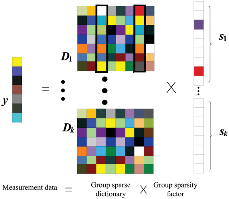
Figure 1: The principle of group sparse representation
In Fig. 1, the original data can be represented as a linear combination of multiple dictionary atoms and their corresponding sparse coefficients, which can be expressed as:
3 The Implementation of Disturbance Localization
3.1 Design of Group Sparse Dictionary
When the disturbance is located based on compressed sensing, they are usually realized by solving a circuit equation built for a kind of electrical data [17]. However, the diversity of disturbance types in power systems renders it insufficient to rely solely on one type of electrical quantity data for the localization of various common disturbances [18,19]. Therefore, this study utilizes the admittance matrix, impedance matrix, and power variation matrix to construct a group sparse sub-dictionary within the framework of compressive sensing.
1. Current as the observation information
When utilizing present data as observational inputs for disturbance localization purposes, the construction of the loop current equation proceeds as follows:
where M represents the number of nodes in the power system where PMUs are installed. The branch current and the node voltage can be expressed as:
where
In the context of three-phase symmetrical disturbances, the power system does not exhibit negative-sequence or zero-sequence components. Similarly, zero sequence components do not exist in asymmetrically grounded disturbances. However, positive sequence components are consistently present in all types of power system disturbances, which can be solved by the following equation:
Based on Eqs. (7) and (6) can be rewritten as follows:
where
2. Voltage as the observed information
According to Eqs. (5) and (8),
where
Nevertheless, numerous intricate computations can result in extended and suboptimal solution durations. Consequently, Eq. (9) remains valid when the absolute value is applied to it, whereby the voltage and impedance are considered as magnitudes. Under these conditions, the solved vector pertains to the amplitude of the variation in positive sequence node current, encompassing the essential information. Additionally, the influence of phase angles on the calculations is eradicated, leading to diminished computational workload and reduced errors. Eq. (9) undergoes the following transformation:
3. Power as the observed information
In the power system, the load power equation can be expressed as follows:
Based on this, the sparse reconstruction model can be constructed as follows:
where i branches can be observed by all PMUs. When j loads are disturbed, respectively,
Due to the limitations in applicability and accuracy when employing only a single electrical quantity as an observation metric, this paper opts to utilize the aforementioned three electrical quantities as observation metrics for designing an overcomplete disturbance dictionary for localization purposes. By combining Eqs. (8), (10), and (12), the group sparse model can be constructed as follows:
where
3.2 The Reconstruction of Disturbance Measurement Data
During the reconstruction process of compressed sensing, several prominent methods that are frequently utilized include Gradient Projection, Homotopy, Iterative Shrinkage-Thresholding (IST), Proximal Gradient, and Augmented Lagrange Multiplier (ALM) [20]. These techniques are chosen due to their efficacy and reliability in handling compressed sensing reconstruction tasks.
In the domain of IST algorithms, advancements in reconstruction algorithms primarily stem from developments based on Orthogonal Matching Pursuit (OMP) [21]. This paper adopts the Generalized Orthogonal Matching Pursuit (GOMP) reconstruction algorithm to solve the group sparse model [22]. Initially, each column of every sub-dictionary in the group sparse dictionary D undergoes an arithmetic squaring operation with the measurement data y. Subsequently, the K columns exhibiting the highest arithmetic squared values are selected to determine the optimal matching atoms. Regrettably, due to the similarity among sparse dictionary atoms, this approach suffers from limited discrimination in match-making, restricting its applicability in denoising tasks.
This paper proposes a Jaccard-generalized orthogonal matching pursuit reconstruction algorithm (J-GOMP) is proposed to address the group sparse model by incorporating the Jaccard coefficient as a substitute for the conventional inner product computation within the algorithm, thereby enhancing its effectiveness and accuracy. This enhancement effectively addresses the challenge of selecting dictionary atoms when the angle between the measurement data and multiple dictionary atom matching vectors is identical, thereby improving dictionary atom identification capability. The calculation process of the Jaccard coefficient is as follows:
Within the context of this paper, a residual threshold value is defined to discern the termination status of iterations. This approach facilitates the efficient convergence of the algorithm throughout the iterative procedure. The parameter denoted as
where a and d are constants.
The procedure of the J-GOMP algorithm unfolds as outlined below:
1) Input: The measurement data vector y, the sparsity parameter Kc for the group sparse sub-dictionary Dk.
2) Initialization phase: Initialize the residual vector as per
3) In accordance with
4) Update the index set using
5) Update the residual signal:
6) Make an iteration decision: Terminate the algorithm if the condition in
7) Output the estimated sparse signal vector, denoted as s.
3.3 Auxiliary Criterion of Disturbance Position
In this paper, we observe the current, power, and voltage cascades and combine the disturbance-complete dictionary reconstruction group sparse vectors to determine the disturbance nodes. The grouping of coefficients corresponding to different categories of sub-sparse dictionaries is known according to the basic principles of information theory: If the information entropy of an observation is slighter, the more information the observation can provide, the higher the weight it takes, and the more intense the influence on the disturbance location in the whole.
3.3.1 Evaluation of Disturbances
In analyzing the amplitude distortion of the variables, the data before the disturbance time t and the data after the disturbance time t are taken for analysis. The amplitude of the disturbance component at the j measurement point is
where
The distortion of the disturbance component before and after the disturbance of the j measurement point is obtained. The calculation formula is shown in Eq. (17).
According to the methods above, the distortion degree of the disturbance component of n measurement points is obtained as
where
Based on the above analysis, the relative disturbance degrees of three categories are obtained for n sets of measurement data, and the evaluation matrix can be obtained as follows:
where
3.3.2 Calculating the Weights of Each Class
The entropy weighting method is an objective assignment method [23]. Its specific calculation steps are as follows:
1. The assessment matrix is standardized to ensure the accuracy of the calculation results, and the calculation formula is shown in Eq. (20):
where
The expression of the standardized evaluation matrix
2. In order to improve the accuracy of information entropy, it is necessary to calculate the relative disturbance proportion of each measured node under a certain index, as follows.
To improve the accuracy of the information entropy, it is necessary to calculate the assigned weight. Under the s indicator, the weight of the relative disturbance of the a set of observations to that indicator is
where s is the index category, and a is the node number.
3. From the theory related to information entropy, the information entropy of various categories can be calculated by Eq. (23), as follows:
4. The weight of each class can be calculated by Eq. (24), as follows:
The weights of each class of sub-dictionary for sparse representation are calculated according to the entropy weighting method. The weight of each class indicates the amount of disturbance information contained. It can be used as a criterion of disturbance location to assist the compressed perception localization results in determining the disturbance location. Due to the different classes of the sparse sub-dictionary of the compressed sensing group, the sparse coefficients obtained from the process of reconstruction can be divided into three parts. If there exists more than one part in which the sparse node coefficients show the same trend in magnitude, the node is a suspected disturbance node, otherwise, the disturbance location is further analyzed by combining the weights.
3.4 The Process of Disturbance Localization
The disturbance location process outlined in this study encompasses several crucial steps: The acquisition of disturbance data, the development of a group sparse dictionary, the reconstruction of compressed sensing, and the identification of disturbance positions using the entropy weight method. These steps are illustrated in Fig. 2, providing a comprehensive and structured framework for the disturbance location process.
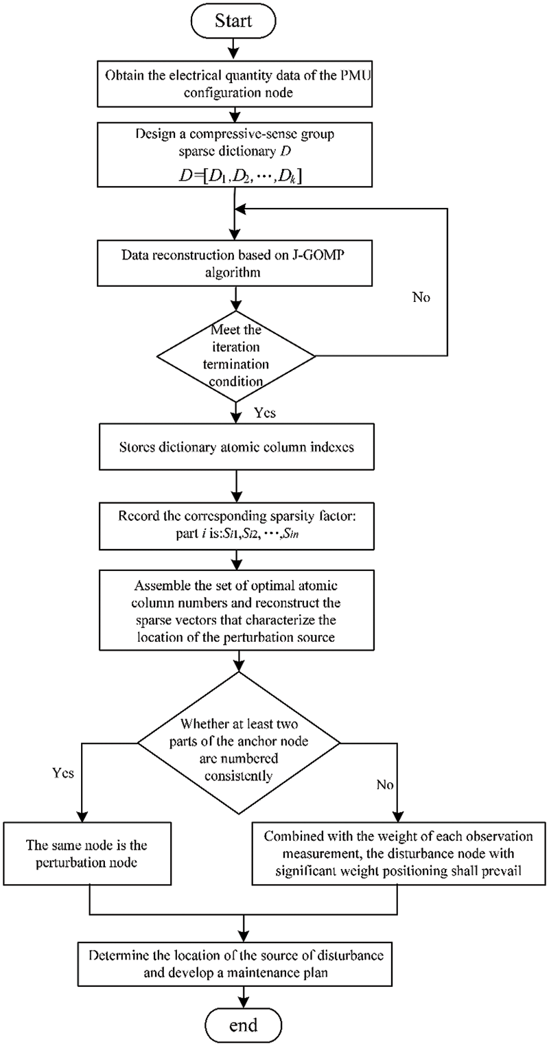
Figure 2: The process of disturbance localization
In this paper, Eq. (25) is used to calculate the accuracy of disturbance localization, as follows:
where Ppp is accurate positioning and Ppd is positioning deviation, it can be concluded that Ppa increases with Ppp while Ppd remains constant.
In order to verify the correctness of the proposed method, the IEEE 39-node system model is built by the PSCAD/EMTDC simulation platform, as shown in Fig. 3. By configuring PMUs at nodes marked with triangles, the number of observed branches of PMUs accounted for 54.3% of the total branches. Since it is rare for multiple disturbances to occur at the same time, this paper only considers the case where a single disturbance occurs.
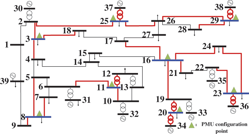
Figure 3: Simulation model of IEEE 39 nodes
4.1 Localization Results of Cut-Off Generator Disturbance
In Fig. 3, there are ten generators. In this paper, the cut-off disturbance of the No. 30 generator is analyzed. After the disturbance occurs, the sparse coefficients of each class were obtained by reconstruction of the J-GOMP algorithm based on PMU observation data and group sparse complete dictionary D. When sparsity K c= 5, the localization results of cut-off generator disturbance are shown in Fig. 4.
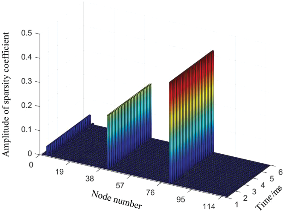
Figure 4: The cut-off generator disturbances of localization results
The localization outcomes depicted in Fig. 4 are segmented into three distinct sections, with each segment comprising 39 numerical values. The initial portion of localization results is associated with nodes 4, 6, and 23, while the subsequent segment correlates the number 42 with node 3. Furthermore, in the third segment, number 81 is identified to again correspond to node 3. In alignment with the principles elucidated in Section 3.4, the identification of a disturbed node requires convergence of localization results from at least two segments on the same node. Notably, based on the analysis presented in Fig. 3, the generator in closest proximity to node 3, identified as Generator No. 30, is deduced to be experiencing a disturbance, thus corroborating the simulated scenarios anticipated.
In the domain of data transmission, the presence of noise interference is an inevitable challenge. Consequently, this paper’s proposed method for disturbance localization is evaluated in terms of its immunity to noise interference. Specifically, the localization of the perturbed cut-off generator is scrutinized following the introduction of Gaussian white noise with a signal-to-noise ratio of 30 dB to all measurement data. The impact of noise on disturbance localization is delineated through the presentation of results in Table 1.
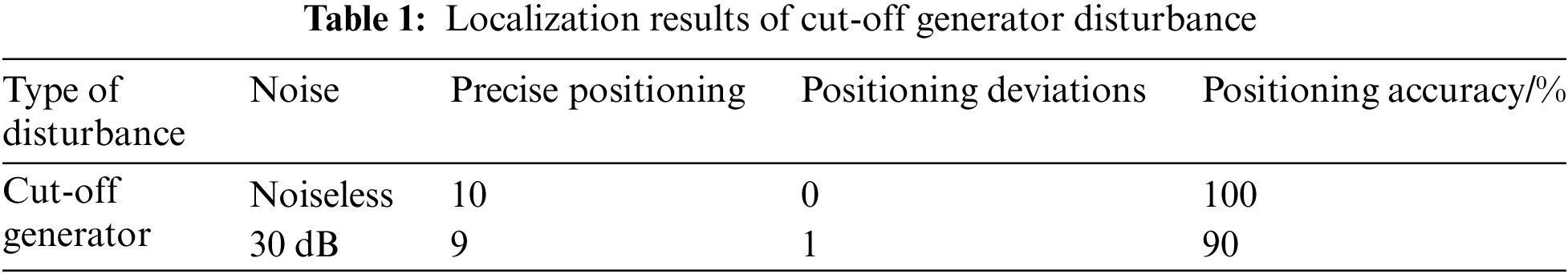
The tabulated findings depicted in Table 1 reveal that the precision of identifying the disturbance in the cut-off generator achieved a rate of 100% under noise-free conditions. Following the introduction of Gaussian noise, the accuracy marginally decreased to 90%. Evidently, the methodology proposed in this study exhibits a notable capacity to mitigate the deleterious effects of noise interference. While the introduction of noise does have an impact on the accuracy of disturbance localization, the observed diminishment in accuracy post-noise-inclusion is deemed negligible in magnitude, indicating the method’s resilience to noise-induced fluctuations.
4.2 Localization Results of Cut-Off Load Disturbance
There are a total of 19 node connection loads in Fig. 3. The disturbance localization experiment was carried out after cut-off at 30%, 50%, and 100% of the capacity of 19 loads, respectively. Taking the localization result of load No. 4 capacity 100% removed as an example for analysis, the localization result is shown in Fig. 5.
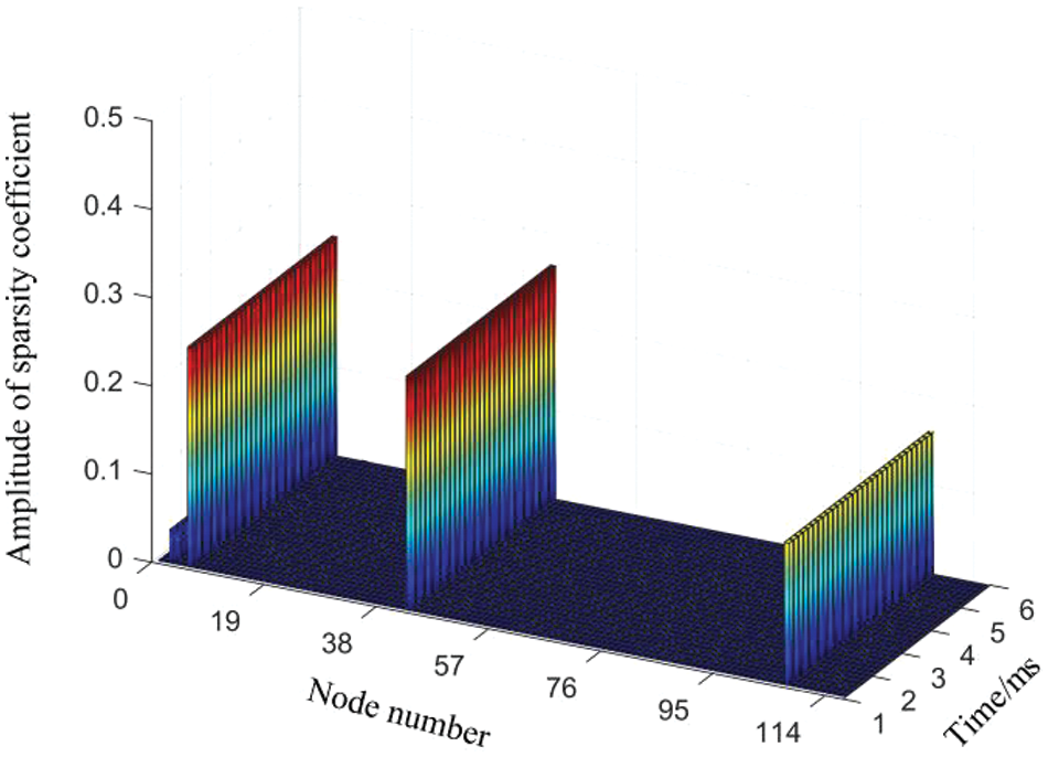
Figure 5: Location results of cut-off load No. 4 disturbance
As shown in Fig. 5, the localization results in the first part correspond to nodes No. 3, 6, and 11, and in the localization results of the second part, the number 43 corresponds to node 4. In the location result of part 3, number 107 corresponds to node 29 too. As can be seen from Fig. 3, nodes 3, 4, and 29 in the power grid are all connected with loads. The localization results of the three parts point to different nodes. Therefore, further analysis should be made based on the weight at this time. The weight of each class is shown in Table 2:
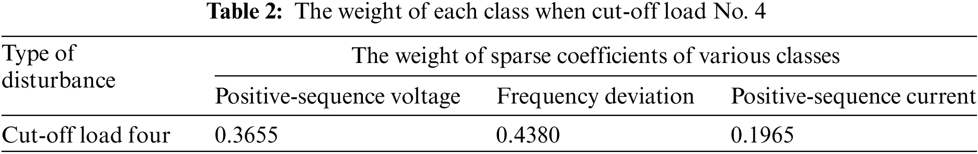
As shown in Table 2, the maximum weight of power is 0.4380. Therefore, the location results of the second part shall prevail. The second part is positioned with the number 45, and the corresponding node number is 4, so set node 4 as a disturbance node. Determine that the location where the disturbance occurs is load four, which is consistent with the set disturbance position and is accurately positioned.
After noise is added to the analysis of the localization results of cut-off load disturbance are shown in Table 3:
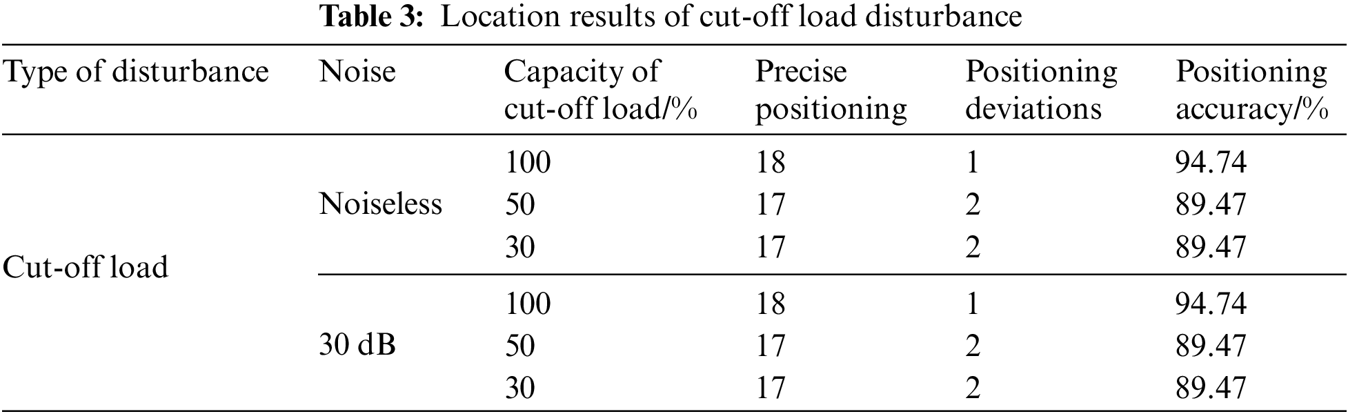
As shown in Table 3, in the location results of cut-off load disturbance, the cut-off load capacity varies, which affects the accuracy of location disturbance, but the variation is slight. The noise will affect the observed data but does not impact the accuracy of location disturbance.
4.3 Localization Results of Short-Circuit Disturbances
The short-circuit disturbance is divided into busbar short-circuit disturbance, and inter-node short-circuit disturbance. To verify the accuracy of the method in this paper for locating short-circuit disturbance, node number 23 and branches 23-24 are set to have short-circuited disturbance, respectively, and the locating results are shown in Figs. 6 and 7.
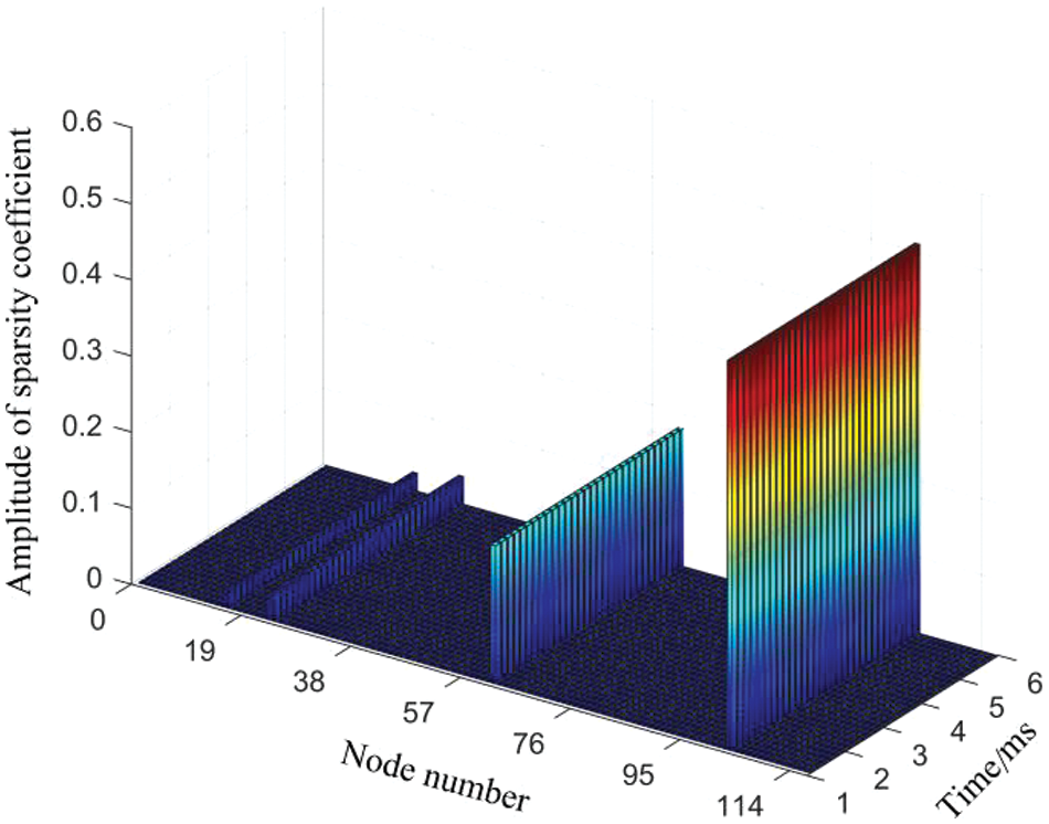
Figure 6: Location results of short-circuit disturbance in node 23
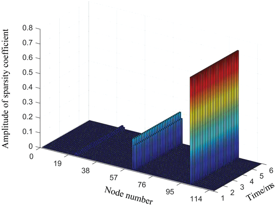
Figure 7: Location results of short-circuit disturbance in branches 23–24
As shown in Fig. 6, the first part of the location corresponds to nodes 16, 23, and 24; the second part of the location is 62, corresponding to node 23; the third part of the location is 103, corresponding to node 25. both the first and second parts of the location results point to node 23, which can be identified as a troubled node.
As depicted in Fig. 7, the initial segment of the location corresponds precisely to node numbers 23 and 24. Subsequently, the second segment of location numbers 62 and 63 is associated with nodes 23 and 24, respectively. Finally, the third segment of location number 101 corresponds exclusively to node 23. The results of all three parts of the location point to node 23, and the results of both parts of the location point to node 24, so it can be concluded that a disturbance has occurred between node 23 and node 24.
The determination of the location of short-circuit disturbances involves the following methodologies: When the location results are the same at least two parts and only one node has a sparse value that is not 0, the node is a disturbance node. When the location results are the same in at least two parts, and the corresponding sparse values of two nodes are not 0 and adjacent, the region between the two nodes is the disturbed region. When the location results of the three parts are different and the corresponding sparse values are not 0 and not adjacent, the position of disturbance is determined by further analysis combined with weight.
In the case of AB-20
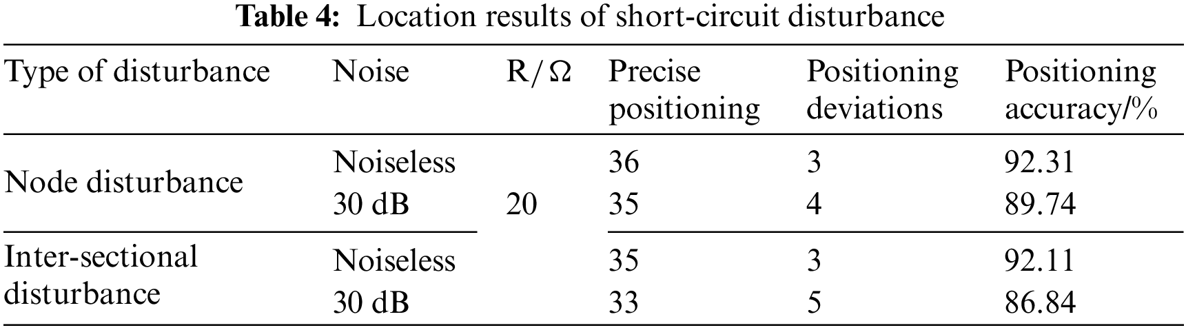
As shown in Table 4, the localization result of node disturbance is 92.31% when there is no noise; the accuracy of the inter-node disturbance localization result is 92.11%. Upon the introduction of Gaussian white noise with a signal-to-noise ratio (SNR) of 30 dB, it can be found that the localization results are still highly accurate. Therefore, the method in this paper can meet the needs of practical applications.
4.4 Comparison with Similar Algorithms
In order to better reflect the superiority of the proposed method, the proposed method is compared with the localization results in reference [8] and reference [10], as shown in Table 5:
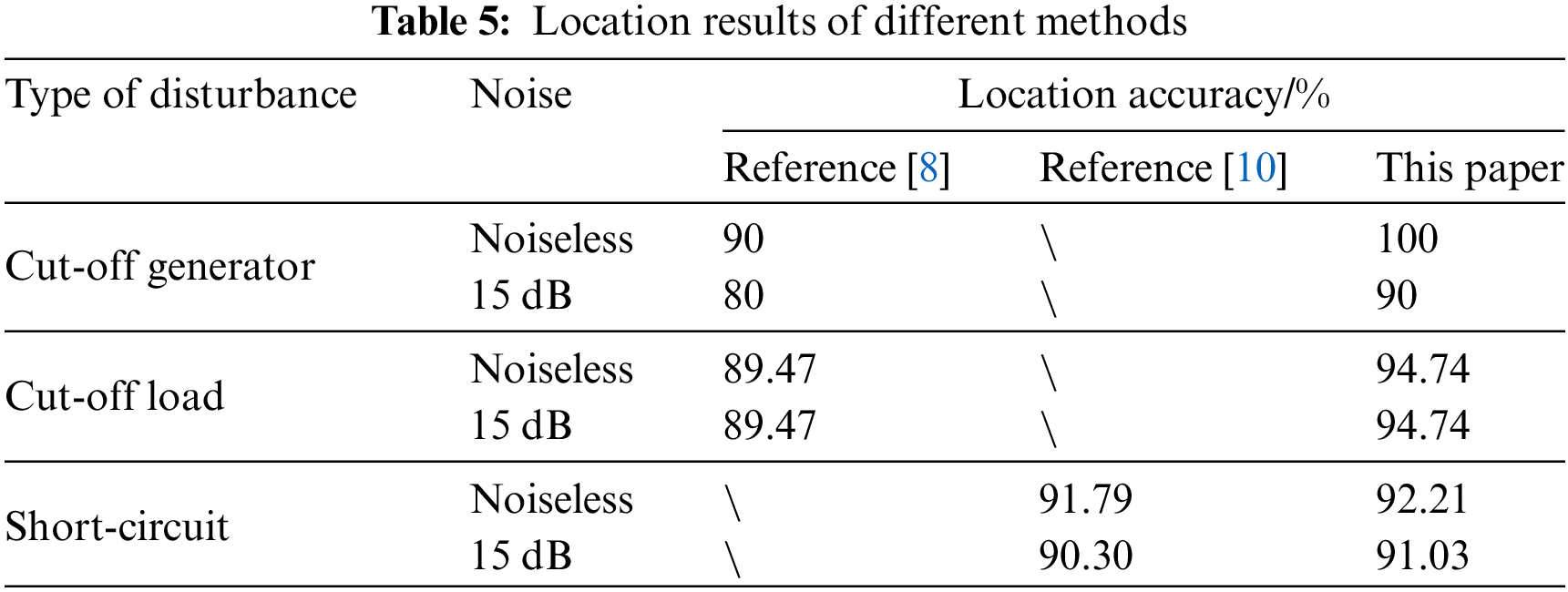
As demonstrated in Table 5, the presence of measurement noise reveals the superior performance of the proposed algorithm in comparison to the referenced methods. Specifically, for cut-off generator disturbances, the localization accuracy of the proposed algorithm stands at 90%, surpassing the reference [8] by a margin of 10%. Similarly, for cut-off load disturbances, the localization accuracy of the proposed algorithm reaches 94.74%, exceeding the reference [8] by 5.27%. Furthermore, in the case of short-circuit disturbances, the proposed algorithm in this study exhibits a localization accuracy of 91.03%, which is approximately 0.7% higher than that reported in reference [10], attributed to the distinct disturbance characteristics. In addition, compared with the noiseless scene, the disturbance localization accuracy of the proposed algorithm hardly changes. Based on the above analysis, it is verified that the proposed method has high localization accuracy for common disturbances and certain anti-noise abilities.
This paper conducts an in-depth analysis of disturbance characteristics within the power system and introduces a group sparse dictionary based on the compressive sensing paradigm derived from the node admittance matrix, node impedance matrix, and node power change matrix. Subsequently, a novel disturbance localization methodology for power systems, leveraging group sparse representation within compressive sensing, is presented, showcasing the following merits:
(1) By scrutinizing the sparse distribution profiles aligned with the positive sequence voltage, frequency variations, and positive sequence current subsequent to a disturbance event, precise disturbance localization is realized, thereby simplifying the detection of disturbance locations. This approach is conducive to pinpointing various commonplace disturbances and exhibits resilience against fluctuations induced by load variations and measurement noise.
(2) A refined version of the conventional GOMP algorithm is proposed, integrating the Jaccard coefficient to replace the vector inner product operation during the matching and tracking stages. This enhancement enhances the algorithm’s ability to identify sparse dictionary atoms, thus augmenting the accuracy of disturbance localization significantly.
Moving forward, the forthcoming research endeavors of this project will be focused on investigating the optimal configuration strategy for PMUs to enhance power system disturbance localization. This includes refining the placement and quantity of PMU installations to streamline the disturbance localization process, thereby enhancing its efficacy while concurrently mitigating associated equipment costs.
Acknowledgement: None.
Funding Statement: This research was funded by the State Grid Jilin Economic Research Institute’s 2022 Practical Re-Search Project on the Construction of Long-Term Power Supply Guarantee Mechanism in Provincial Capital Cities under the New Situation, Grant Number SGJLJY00GPJS2200041.
Author Contributions: Zeyi Wang and Mingxi Jiao primarily focused on the research of compressed sensing theory. Daliang Wang and Minxu Liu were responsible for programming. Minglei Jiang designed the simulation experiments. He Wang and Shiqiang Li were primarily involved in refining the theory and debugging the simulations.
Availability of Data and Materials: The data that support the findings of this study are available on request from the corresponding author.
Conflicts of Interest: The authors declare that the research was conducted in the absence of any commercial or financial relationships that could be construed as a potential conflict of interest.
References
1. A. S. F. Sobrinho, R. A. Flauzino, L. H. B. Liboni, and E. C. M. Costa, “Proposal of a fuzzy-based PMU for detection and classification of disturbances in power distribution networks,” Int. J. Elec. Power, vol. 94, pp. 27–40, Jan. 2018. doi: 10.1016/j.ijepes.2017.06.023. [Google Scholar] [CrossRef]
2. M. R. Shadi, M. T. Ameli, and S. Azad, “A real-time hierarchical framework for fault detection, classification, and location in power systems using PMUs data and deep learning,” Int. J. Elec. Power, vol. 134, Jan. 2022. doi: 10.1016/j.ijepes.2021.107399. [Google Scholar] [CrossRef]
3. X. D. Deng et al., “Impact of low data quality on disturbance triangulation application using high-sensity PMU measurements,” IEEE Access, vol. 7, pp. 105054–105061, Aug. 2019. doi: 10.1109/ACCESS.2019.2932035. [Google Scholar] [CrossRef]
4. M. S. Ballal and A. R. Kulkarni, “Synergizing PMU data from multiple locations in Indian power grid-case study,” IEEE Access, vol. 9, pp. 63980–63994, May 2021. doi: 10.1109/ACCESS.2021.3074562. [Google Scholar] [CrossRef]
5. K. Jia, B. Yang, T. Bi, and L. Zheng, “An improved sparse-measurement based fault location technology for distribution networks,” IEEE Trans. Ind. Inform., vol. 17, no. 3, pp. 1712–1720, Mar. 2021. doi: 10.1109/TII.2020.2995997. [Google Scholar] [CrossRef]
6. B. Yang, K. Jia, Q. Liu, L. M. Zheng, and T. S.Bi, “Faulted line-section location in distribution system with inverter-interfaced DGs using sparse meters,” IEEE Trans. on Smart Grid, vol. 14, no. 1, pp. 413–423, Jan. 2023. doi: 10.1109/TSG.2022.3186541. [Google Scholar] [CrossRef]
7. H. Yu, C. Ma, H. Wang, W. Liu, Y. Du and X. Bai, “Research on VSC-HVDC fault location method based on compressed sensing (in Chinese),” Acta Energ. Sol. Sin., vol. 41, no. 3, pp. 158–166, Mar. 2020. doi: 10.19912/j.0254-0096.2020.03.021. [Google Scholar] [CrossRef]
8. H. Yu, Y. N. Li, and H. X. Wang, “Disturbance location method of power system based on over-complete reconstruction dictionary design (in Chinese),” Trans. China Electrotech. Soc., vol. 35, no. 7, pp. 1444–1453, Apr. 2020. doi: 10.19595/j.cnki.1000-6753.tces.190451. [Google Scholar] [CrossRef]
9. M. Majidi, M. Etezadi-Amoli, and M. S. Fadali, “A sparse-data-driven approach for fault location in transmission networks,” IEEE Trans. Smart Grid, vol. 8, no. 2, pp. 548–556, Mar. 2017. doi: 10.1109/TSG.2015.2493545. [Google Scholar] [CrossRef]
10. K. Jia, L. Li, Z. Yang, G. Zhao, and T. Bi, “Research on distribution network fault location based on bayesian compressed sensing theory,” in Proc. CSEE, Jun. 2019, vol. 39, no. 12, pp. 3475–3486 (in Chinese). doi: 10.13334/j.0258-8013.pcsee.180705. [Google Scholar] [CrossRef]
11. K. Jia, C. Gu, T. Bi, Y. Chen, and Z. Ren, “Research on the compressed sensing based fault location within the collection system of a large-scale photovoltaic power plant,” in Proc. CSEE, Jun. 2017, vol. 37, no. 12, pp. 3480–3489 (in Chinese). doi: 10.13334/j.0258-8013.pcsee.161154. [Google Scholar] [CrossRef]
12. F. Aminifar, A. Khodaei, M. Fotuhi-Firuzabad, and M. Shahidehpour, “Contingency-constrained PMU placement in power networks,” IEEE Trans. Power Syst., vol. 25, no. 1, pp. 516–523, Feb. 2010. doi: 10.1109/TPWRS.2009.2036470. [Google Scholar] [CrossRef]
13. Y. J. Yan et al., “Application of random matrix model in multiple abnormal sources detection and location based on PMU monitoring data in distribution network,” IET Gener. Trans. Dis., vol. 14, pp. 6476–6483, Dec. 2020. doi: 10.1049/iet-gtd.2020.0755. [Google Scholar] [CrossRef]
14. H. U. Banna, S. K. Solanki, and J. Solanki, “Data-driven disturbance source identification for power system oscillations using credibility search ensemble learning,” IET Smart Grid, vol. 2, pp. 293–300, Jun. 2019. [Google Scholar]
15. A. Jalilian and S. Samadinasab, “Detection of short-term voltage disturbances and harmonics using μpMU-based variational mode extraction method,” IEEE T. Instru. Meas., vol. 70, Feb. 2021. doi: 10.1109/TIM.2021.3075744. [Google Scholar] [CrossRef]
16. Q. R. Jiang et al., “Design of compressed sensing system with probability-based prior information,” IEEE Trans. Multimedia, vol. 22, no. 3, pp. 594–609, Mar. 2020. doi: 10.1109/TMM.2019.2931400. [Google Scholar] [CrossRef]
17. X. Xia, C. He, Y. Lv, B. Zhang, S. Wang, C. Chen, and H. Chen, “Power quality data compression and disturbances recognition based on deep CS-BiLSTM algorithm with cloud-edge collaboration,” Front. Energ. Res., vol. 10, pp. 1–14, Apr. 2022. doi: 10.3389/fenrg.2022.874351. [Google Scholar] [CrossRef]
18. A. Lqbal and T. Jain, “Real-time event detection based on weibull distribution Using synchrophasor measurements for enhanced situational awareness,” IEEE Trans. on Power Systems, vol. 37, pp. 1425–1436, Mar. 2022. doi: 10.1109/TPWRS.2021.3108481. [Google Scholar] [CrossRef]
19. S. Azizi, M. R. Jegarluei, A. S. Dobakhshari, G. Y. Liu, and V. Terzija, “Wide-area identification of the size and location of loss of generation events by sparse PMUs,” IEEE Trans. on Power Delivery, vol. 36, pp. 2397–2407, Aug. 2021. doi: 10.1109/TPWRD.2020.3047228. [Google Scholar] [CrossRef]
20. Z. Wang et al., “A disturbance localization method for power system based on group sparse representation of compressed sensing,” in 2023 IEEE 2nd Int. Conf. Electr. Eng., Big Data Algorithms (EEBDA), 2023, pp. 1084–1089. doi: 10.1109/EEBDA56825.2023.10090771. [Google Scholar] [CrossRef]
21. S. P. Mu et al., “An adaptive MP algorithm for underwater acoustic channel estimation based on compressed sensing,” IEEE Access, vol. 11, pp. 109131–109141, Nov. 2023. doi: 10.1109/ACCESS.2023.3321702. [Google Scholar] [CrossRef]
22. S. X. Shi, B. S. M. Zhu, and X. Z. Dong, “Fault classification for transmission lines based on group sparse representation,” IEEE Trans. Smart Grid, vol. 10, no. 4, pp. 4673–4682, Jul. 2019. [Google Scholar]
23. Y. Xu, J. Xing, Y. Zhang, and H. Li, “Generalized orthogonal matching pursuit for distributed compressed sensing,” Int. J. Innov. Comput., Inf. Control, vol. 11, no. 4, pp. 1441–1456, Jul. 2015. [Google Scholar]
Cite This Article
 Copyright © 2024 The Author(s). Published by Tech Science Press.
This work is licensed under a Creative Commons Attribution 4.0 International License , which permits unrestricted use, distribution, and reproduction in any medium, provided the original work is properly cited.
 Downloads
 Citation Tools