Arc Grounding Fault Identification Using Integrated Characteristics in the Power Grid

1  Introduction

In recent years, to deal with the problems of fault over-voltage and insensitive fault line selection, many urban power grids and large-scale industrial power supply systems have widely adopted neutral small resistance ground operation mode [1–3]. However, there is no arc suppression coil, so the arc energy can not be suppressed under the grounding fault condition. Hence, arc grounding fault, as a special form of grounding fault, has been widely concerned because of its extreme physical characteristics, which can easily lead to line insulation breakdown, system disorder, power supply breakdown, and even electrical fire [4,5].

Arc fault detection methods are mainly divided into two categories, one mainly focuses on the arc fault external characteristics [6–9], such as arc light, arc sound, temperature, and so on. This method mainly detects by setting a sensor at the switch device. However, due to the problems in the setting of detection devices and the randomness of arc occurrence, such detection methods are often limited and inefficient. The other kind of methods mainly focus on the internal characteristics of arc occurrence, such as the time-frequency domain characteristics of fault current and voltage [10–13]. This kind of method has high detection accuracy, wide monitoring range, and fast response speed, so it has become the mainstream identification method in power grid fault detection.

There are many identification characteristics used commonly in arc fault identification [14–17], such as harmonic distortion rate, peak value, kurtosis, euclidean distance, variance, and so on. In reference [14], the harmonic distortion rate and energy value of zero sequence arc current are proposed. Compared with the set threshold, the arc fault can be judged. In reference [15], the Gaussian distribution is used to fit the arc fault signal, the fitting result is compared with the peak value of the fault signal, and the calculated result is compared with the set threshold. In reference [16], the decomposition of arc fault current by fast Fourier transform is proposed. Then the Euclidean distance of the arc fault fundamental frequency current is calculated, and the calculated value is compared with the threshold value. In reference [17], a variety of time-frequency domain features such as kurtosis, variance, and curvature are proposed. The arc fault identification database is formed by using these indexes. In some scenarios, the fault type can be identified effectively by calculating the characteristic index of the fault signal.

Recently, many machine learning algorithms have applied identification characteristics to the detection of fault discrimination and achieved good results, such as K-nearest neighbor [18,19], support vector machine [20–22], random forest algorithm [23–25], fuzzy clustering algorithm [26,27], convolutional neural network [28,29], and so on.

The realization and classification of machine learning methods mainly lie in the input of different feature indexes. For instance, in reference [21], an empirical mode decomposition technique based on the Hurst index is proposed. The collected fault signal is decomposed by this technique. The arc characteristic energy, root mean square, and variance of the processed signal are calculated. The fault discrimination model is obtained by substituting the calculated results into the support vector machine algorithm as the feature criterion. Reference [22] calculates four characteristics of fault current in the time domain: mean current, range current, mean differential current, and current variance. Ten characteristics of fault current in the frequency domain are extracted by the fast fourier transform algorithm. The time domain and frequency domain features were input into a particle swarm optimization-support vector machine as criteria to form a machine learning-based identification model.

However, for the selection of fault feature criteria, most scholars only focus on the time-frequency domain identification features of the fault line signal, while the rich signal features generated by other sound lines are always ignored. Fault line features are not always significant in some special scenarios. For example, the commonly used “zero off” feature of fault line current signals is not obvious when the arc dissipated power is small, and the zero off period is very short, which leads to a significant reduction in the fault recognition rate. Nevertheless, at this time, the sound line features are still relatively rich and can still be used as the basis for fault identification.

Given the above problems, this paper presents an arc grounding fault identification method based on integrated characteristics. When a grounding fault occurs, it uses the signal characteristics of not only the fault line but also other sound lines as the fault identification index, so it can effectively identify arc faults in various scenarios. Compared with the existing methods, the proposed method has more advantages when the arc dissipation power is low and the arc “zero-off” is not obvious. Test results indicate that the proposed method has higher accuracy in arc identification.

The rest of this paper is organized as follows: The second section introduces the characteristics of fault lines in arc fault network and the convex hull area used for identification; the third section introduces the formation mechanism of zero sequence current of sound lines and the gradient product and correlation coefficient used for identification; the fourth section introduces the algorithm of machine learning and the selected model; the fifth and sixth sections include simulation experiment, actual data experiment, analysis and method comparison. Finally, the seventh part summarizes the thesis.

2  Fault Line Characteristics and Identification Index

2.1 Arc and Its Waveform Characteristics

The generation of the arc fault is a dynamic development process, which goes through several cycles of “quenching and burning”. The Mayr model has been widely concerned and applied because of its good performance in simulating arc. According to the Mayr model, the mathematical model of arc is expressed as:

1gdgdt=dlngdt=1μ(Ud×Idph−1)(1)

where g is the arc conductance; μ is the time constant of the arc; Ud is the arc voltage; Id is the arc current; and Ph is the dissipated power of the arc.

When the arc current waveform crosses zero, the input power generated is less than its own dissipation power. At this time, UdId<Ph, which causes the energy generated by the arc to be insufficient to maintain the burning state, so it goes into an arc quenching state. The waveform of the arc current shows a “zero off” state. With the sharp reduction of the current, the arc voltage rises rapidly, and the waveform of the arc voltage shows a “peak” shape. After that, the input power of the arc is gradually greater than the dissipated power, and the arc burns violently again and enters a new arc state. At this time, the arc current waveform begins to appear sinusoidal. With the recovery of the arc current, the arc voltage decreases rapidly and approaches a stable state, showing a saddle-like shape in the waveform. The above process is shown in Fig. 1.

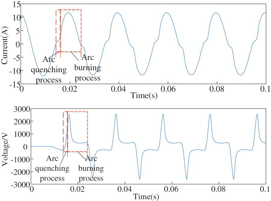
Figure 1: The waveform graphs of the arc current and voltage

2.2 Convex Hull Index of the Fault Line

According to the above analyses, fault identification can be carried out by using fault line current characteristics so that some indexes can be set to check it.

The convex hull is a graphic concept. Relative to a set of points in two-dimensional space, all points are required to be surrounded by a convex polygon, and this convex polygon is the smallest region containing all points.

The zero sequence current waveform of the arc fault line has a zero-off characteristic at zero crossing. So the result obtained by sinusoidal fitting is quite different from the original signal. The zero sequence current waveform of the single-phase grounding fault is very similar to the sinusoidal fitting results. The convex hull algorithm can be used to highlight this difference.

The signal of fault zero sequence current within one cycle is selected as the abscissa. The signal array after sinusoidal fitting is taken as the ordinate. In the first and second quadrants, the convex hull algorithm is used to construct the smallest convex polygon which can contain all points. By the convex hull area, the arc grounding fault and the non-fault state can be distinguished.

3  Sound Line Characteristics and Identification Index in Fault Scenario

In the neutral effective grounding power supply system, once the grounding fault occurs, the zero sequences current waveform under arc fault shows the character of “zero off”, while the zero sequences current waveform under non-fault state still shows the sinusoidal character. Most scholars have used this characteristic to distinguish arc grounding fault and non-fault state. However, when the arc dissipated power is small, the “zero off” feature in the arc current waveform of the fault line will be not obvious. In this situation, the detection methods only based on the arc current waveform characteristics of the fault line will face severe challenges and even fail.

Where l1,l2,l3 represent three arc curves with increasing dissipated power. It can be found from Fig. 2 that when the dissipated power is reduced, the zero-off period of the zero sequence current waveform becomes significantly shorter. It corresponds to the quenching time becoming shorter and the zero-off period is shortened when the arc passes zero.

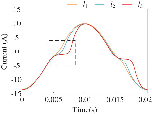
Figure 2: Zero sequence current of arc fault in three cases

3.1 Characteristic Analysis of Sound Lines in the Fault Scenario

In this paper, it is found that the waveform characteristics of sound lines in fault scenarios also have characteristics. In the zero sequence current waveform of the sound lines, there are also some waveform distortion characteristics at the crest and trough. If the analysis is carried out effectively, the criteria for identifying arc faults can also be selected from it.

When a single-phase grounding fault occurs in the system, unbalanced voltages and fault loops will occur. At this time, the line impedance is far less than the line capacitance-reactance. The zero-sequence simplified network can be represented in Fig. 3.

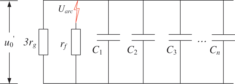
Figure 3: Simplified zero sequence network diagram

In this figure, C1,C2,C3,Cn are the line zero sequence capacitance of different lines, respectively; u0 is the zero sequence voltage.

According to the fault component method and superposition theorem, the power network after the fault can be equivalent to the superposition of the power network before the fault and the fault additional network. Therefore, the voltage at the power supply in the fault-attached network becomes zero after subtracting (before and after the fault), and the phase voltage fault component at the fault point becomes Δu after subtracting, as follows:

Δu=uarc−uϕ(2)

where the time domain expression of arc voltage (uarc) in Eq. (3) is

uarc=(UT0+rI)[L0−D2(1+sinωst)](3)

where UT0 is the arc voltage gradient; r is the arc resistance; L0 is the reference arc length; D is the maximum change of arc length of arc; ωs is the signal angular frequency.

The pre-fault phase voltage (uϕ) in Eq. (4) is

uϕ=UMsinωt(4)

where UM is the maximum voltage of the system during normal operation; ω is the system angular frequency.

The zero sequence current of a sound line can be expressed as

is=CndΔudt=Cnd(uarc−uϕ)dt(5)

Substitute Eqs. (3) and (4) into Eqs. (5) and (6) is obtained as

is=Cndu0dt=Cn(duarcdt−ωUMcosωt)(6)

It can be seen from Eq. (6) that there is a derivative relationship between the zero sequence current of the sound line and the zero sequence voltage of the arc. A group of arc fault voltage signals and zero sequence current signals of sound lines are obtained through experiments, as shown in Fig. 4.

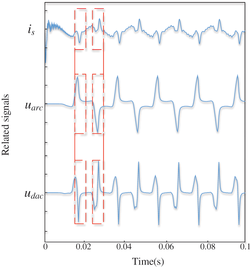
Figure 4: Arc voltage and zero sequence current in sound lines

In Fig. 4, is, uarc and udac represent the zero sequence current of the sound line, arc fault voltage, and arc fault voltage derivative, respectively. It can be seen that La has obvious distortion at the crest and trough, and La corresponds to Lb distortion exactly. La and Lc also have obvious similarities here.

These characteristics prove that the arc transmits the arc fault characteristics to the sound line through Eq. (6). Therefore, the arc fault can be judged by utilizing the characteristics of sound line currents.

3.2 Gradient Product Index of Sound Lines in the Arc Fault Scenario

According to the analysis in the above section, it can be seen that the zero sequence current waveform of the sound line has a distortion section at the crest and trough, and the index, gradient product, can be designed to detect it.

The gradient product can measure the growth direction, growth rate, and transformation rate of the directional derivative of a function at a certain point or a certain segment. Its mathematical expression is as follows:

dk=−sign(Lk×Rk)(7)

where Lk and Rk are the left and right gradients, Lk=Zk−Zk−bc, Rk=Zk+bc−Zk; bc is the step size; dk is the gradient product.

The zero sequence current waveform of the sound line has an oscillating distortion section at the crest and trough, and a relatively large gradient product value can be obtained by calculation. The gradient product values of other gentle regions are relatively small.

However, for the non-fault state, the zero sequence current waveform of the sound line does not have the characteristics of oscillation and distortion, and the waveform changes continuously sinusoidal at the crest and trough, and the gradient product values are always small.

3.3 Correlation Coefficient Index of Sound Lines in the Fault Scenario

After the arc ground fault occurs, due to the transmission and energy supply of the voltage at the fault point, there are great differences between the zero sequence current waveform and the sine curve at the peak and trough of the sound line. According to the similarity, the correlation coefficient index can be set to distinguish.

The correlation coefficient can measure the degree of correlation between the two variables, and its value is between [−1,1]. The closer the value is to 1, the more positive correlation between the two signal variables is and the more similar the signals are. The closer the value is to −1, the more negative correlation is shown between the two signal variables. The correlation coefficient is calculated by the following formula:

gX,Y=cov(X,Y)σXσY=1m−1∑n=1m(Xn−X¯σX)(Yn−Y¯σY)(8)

where the cov is the covariance matrix of two signal variables; σ is the standard deviation of a variable; m is the total sampling point signal number; X is the zero sequence current data at the peak and trough of the sound line; Y is the sinusoidal data for calculation.

According to the revelation of Eq. (6), the zero-sequence voltage signal of the bus is fitted and derived, so as to obtain the sinusoidal data (Y) involved in the correlation analysis.

4  Fault Identification of Integrated Information Features

4.1 Establishment of Fault Arc Identification Sample Database

Through the above characteristic analysis, the convex hull index, the gradient product index, and the correlation coefficient index can be selected as the base characteristic parameters of the machine learning sample database.

To further ensure the accuracy of these basic characteristic parameters, on this basis, the basic characteristic parameters are taken as signal variables, and standard deviation, variance, and other conventional time-frequency domain characteristic parameters are set as auxiliary characteristic parameters, to further improve the establishment and learning scope of the fault arc identification sample database from multiple angles and dimensions.

The fault diagnosis model based on this sample database can greatly improve the accuracy of identifying fault types.

4.2 Logistic Regression Diagnostic Model

In many existing machine learning algorithms, logistic regression has been widely used in fault identification and classification, because of its ability to solve small samples, its simple structure, parallelization, superior model type recognition, and low generalization error rate.

Its essence is the combination of regression equation and sigmoid function [30,31]. The function of sigmoid is to convert the results predicted by the linear regression model to [0,1] in the form of probability.

The general output expression of the regression equation is: y=ωTzi+b, where ω is the weight vector; zi is the input vector; zi={(x1,y1),(x2,y2),…,(xn,yn)}, b is the optimal parameter.

The sigmoid function expression is:

y=11+e−z(9)

Substituting the regression output equation is the logistic regression expression:

y=11+e−z=11+e−(ωTx+b)(10)

The above expression can be deformed to obtain:

{lnp(y=1|x)p(y=0|x)=ωTx+bp(y=1|x)=exp(ω⋅x)1+exp(ω⋅x)p(y=0|x)=11+exp(ω⋅x)(11)

The loss parameter of the logistic regression is:

j(ω)=(−1n∑i=1n[yi(ωTx+b)−ln(eωTx+b+1)])(12)

The classification interval can be set. When the calculated probability is larger than 0.5, the model predicts that an arc grounding fault occurs in the system, and the output is 1. Conversely, when the calculated probability is less than 0.5, the system is predicted to have a non-fault state and the output is 0. Therefore, according to the input vector, the fault type can be determined by the output value of the model.

4.3 Global Algorithm Flow

The overall identification process of this work is shown in Fig. 5. Firstly, by designing multiple groups of experiments, the characteristic parameters of the experimental group were calculated to form the characteristic parameter database. Before this step, these experimental procedures were artificially set up. And the fault lines and sound lines are also artificial and known. These experimental data are used as training models. Then the fault discrimination model based on the logistic regression was formed by learning the database. In fact, when a fault occurs in the grid, all the line signals are detected and collected by the system. In the step of fault identification, the signal with the largest value in the detected zero sequence current of the line is judged as the suspected fault line signal, and the rest of the signal is judged as the suspected sound line signal. For these suspected input signals, the characteristic parameters are calculated. Then the characteristic parameters are substituted into the discrimination model to determine whether arc fault occurs according to the output label.

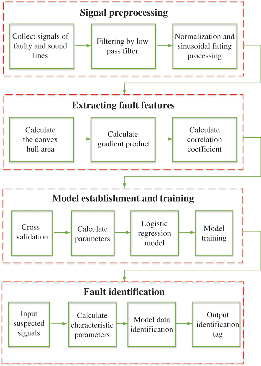
Figure 5: Arc grounding fault recognition algorithm flow chart

5  Tests Verification and Comparisons

5.1 Simulation for Obtaining Feature Parameters

To verify the effectiveness of the proposed method, the simulation model as shown in Fig. 6 is built in Simulink soft for testing.

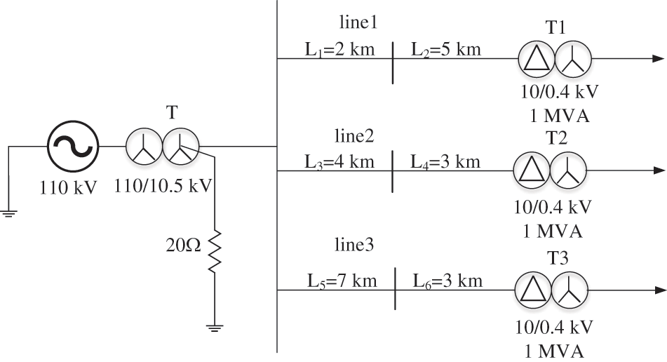
Figure 6: Power grid simulation model

The simulation system is grounded by resistance at the neutral point. The system frequency is 50 Hz. It contains three lines. The lengths of the lines are 7, 7, and 10 km, respectively. The Mayr arc model is used for simulating the arc fault model. The fault is set at reference zero time (0 s). The sampling frequency is set to 6000 Hz. Non-fault state and arc grounding faults are respectively simulated and tested.

(1) Arc grounding fault

An arc grounding fault is simulated. The specific parameters are set as follows: τ = 6 × 10−4, Ploss = 2 × 103 W, g(0) = 1000 S. Other fault conditions are consistent with those set in the previous simulation experiment. Zero-sequence currents of sound lines are collected. The sinusoidal fitting curve curve, convex hull diagram, gradient product curve, and correlation coefficient curve are drawn. The results are shown in Fig. 7.

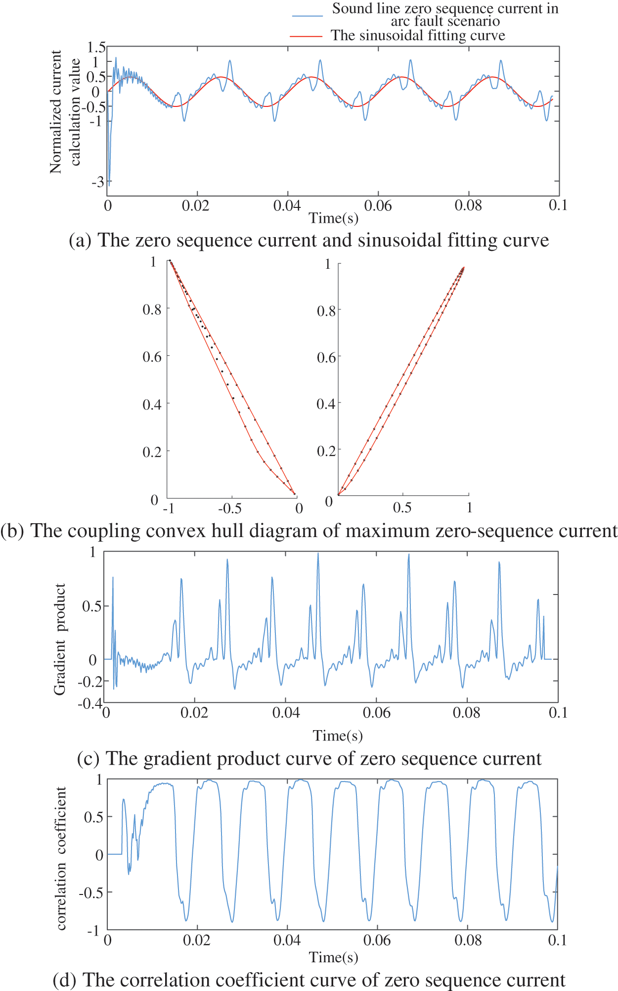
Figure 7: Simulation results of arc grounding faults

The convex hull area value in this example is 0.0672 on the left and 0.0487 on the right, the gradient product value is 0.5661, and the correlation coefficient value is −0.8416. The variance of auxiliary feature parameters is 0.2031 and the standard deviation is 0.4507. They are also sent to the logistic regression diagnostic model as the basic and auxiliary feature parameters.

(2) Non-fault state

Set the three insulation asymmetries of the system, and collect the maximum zero sequence current and the other zero sequence currents in the line. The sinusoidal fitting curve corresponding to the zero-sequence voltage is drawn. They have been converted to the same order of magnitude. The convex hull diagram, the gradient product, and the correlation coefficient curve are shown in Fig. 8.

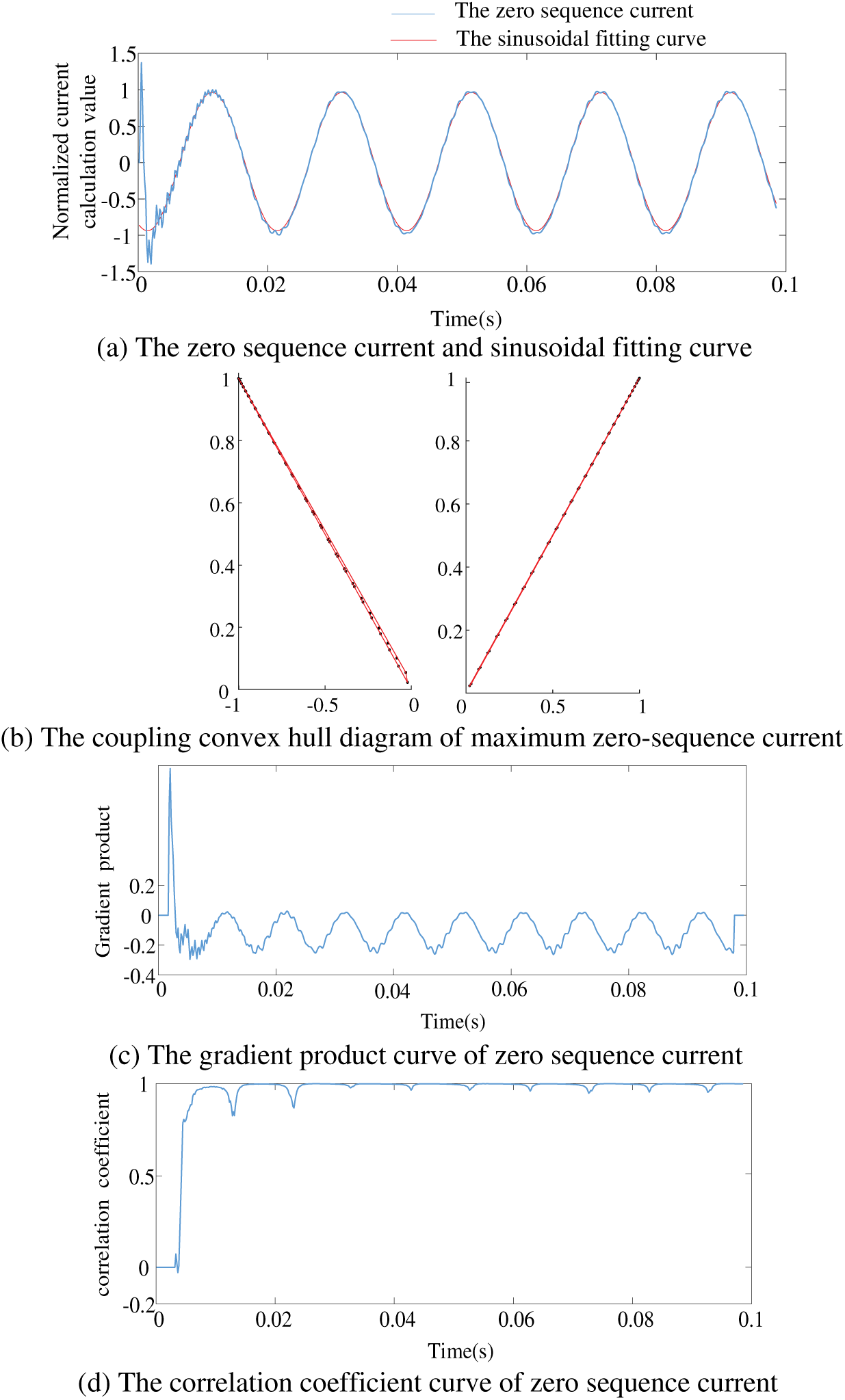
Figure 8: Simulation results of non-fault state

According to the proposed indexes, after half a power frequency cycle, the calculated convex hull area value (left 0.0114, right 0.0028), the maximum gradient product value (in this case 0.0279), and the minimum correlation coefficient value (in this case 0.8245) are utilized as the basic characteristic parameters in the logistic regression diagnostic model. Additionally, the variance (0.4483) and the standard deviation (0.6695) are utilized as the auxiliary feature parameters.

5.2 Establishment of Training Sample Database

By changing conductor core parameters, insulating layer parameters, shielding layer parameters, and sheath layer parameters of the line, 100 groups of asymmetric non-fault state of three-phase insulation are generated. In addition to the above parameters, the three key parameters of the arc (dissipated power, time constant, and initial arc conductance) are modified for testing. Specifically, the varying range of the dissipated power is 1.5 × 103 W ~ 4 × 103 W, the value of the time constant is 3 × 10−4 ~ 1.2 × 10−3, and the initial arc conductance is 1000 S ~ 4000 S. A total of 100 groups of arc grounding faults are generated for training.

A fault diagnosis sample base based on characteristic parameters is established. The feature vector of the sample library is composed of 4 base feature parameters and 2 auxiliary feature parameters. Category labels are defined in Table 1.

5.3 Test Results and Comparisons

Another 200 groups of samples (100 groups of non-fault state and 100 groups of arc) are simulated for testing. The setting scheme for Parameter parameters is the same as above. The fault groups are distinguished mainly by changing the main experimental parameters. Three existing arc fault identification methods based on fault kurtosis, harmonic amplitude energy, and complementary ensemble empirical mode decomposition features are selected. The test and comparison results are shown in Table 2, which proves the performance and advantages of the proposed method.

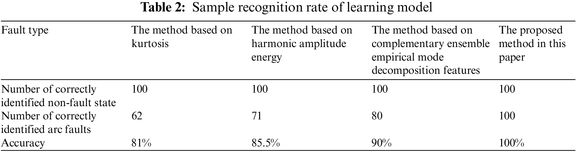
The test results show that the four methods can identify non-fault states effectively, but the methods based on fault kurtosis, harmonic amplitude, and complementary ensemble empirical mode decomposition feature have 38, 29, and 20 groups of error identification for arc grounding faults, respectively. The characteristics of these error groups are all less than 2 × 103 W dissipated power, with short arc zero-off time and inconspicuous zero-off characteristics. A group of identification failure groups is randomly selected and shown in Fig. 9.

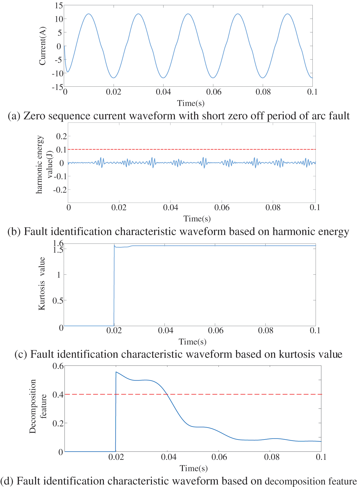
Figure 9: Identification results based on harmonic energy, kurtosis value, and decomposition feature

As shown in Fig. 9a, the zero-off period of the arc fault zero sequence current at this time is very short. The zero-off characteristics are difficult to identify. On this basis, these identification methods are affected to some extent.

The method is based on fault kurtosis by judging whether the kurtosis value of the fault zero sequence current is greater than the threshold value (1.6). As shown in Fig. 9b, the kurtosis value of the arc fault curve is always smaller than the threshold value. The method will misjudge this fault as a non-fault state.

Another method is based on harmonic amplitude energy by judging whether the d2 energy wave after wavelet analysis is greater than the threshold value (0.1). As shown in Fig. 9c, the arc fault value is always smaller than the threshold, this method will misjudge it as a non-fault state.

In the method based on decomposition features, the suspected fault signal is decomposed by complementary empirical mode to obtain many components, and the component with the largest energy difference is selected as the signal source, and then the time-frequency domain characteristics are used to calculate, and the signal is judged as non-fault when it exceeds the threshold value (0.4). As shown in Fig. 9d, there are parts of decomposition features that are greater than the threshold value, this method will misjudge it as a non-fault state.

As can be seen from Table 2, the proposed method can well identify arc grounding faults and non-fault states. In some cases where the arc fault zero-off characteristic is not obvious, this model can also adapt and identify fault types. Under the influence of basic feature parameters and auxiliary feature parameters, the accuracy and efficiency of the proposed method are guaranteed. The detailed identification results of the proposed method are shown in Fig. 10.

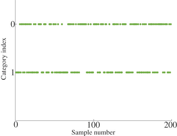
Figure 10: Identification results of the proposed method for 200 samples

6  Experimental Verification

To simulate the arc fault in the actual working conditions as truly as possible, a power grid experimental test platform based on the national standard GB/T31143 and UL1699 is shown in Fig. 11. The experimental parameters are shown in Table 3.

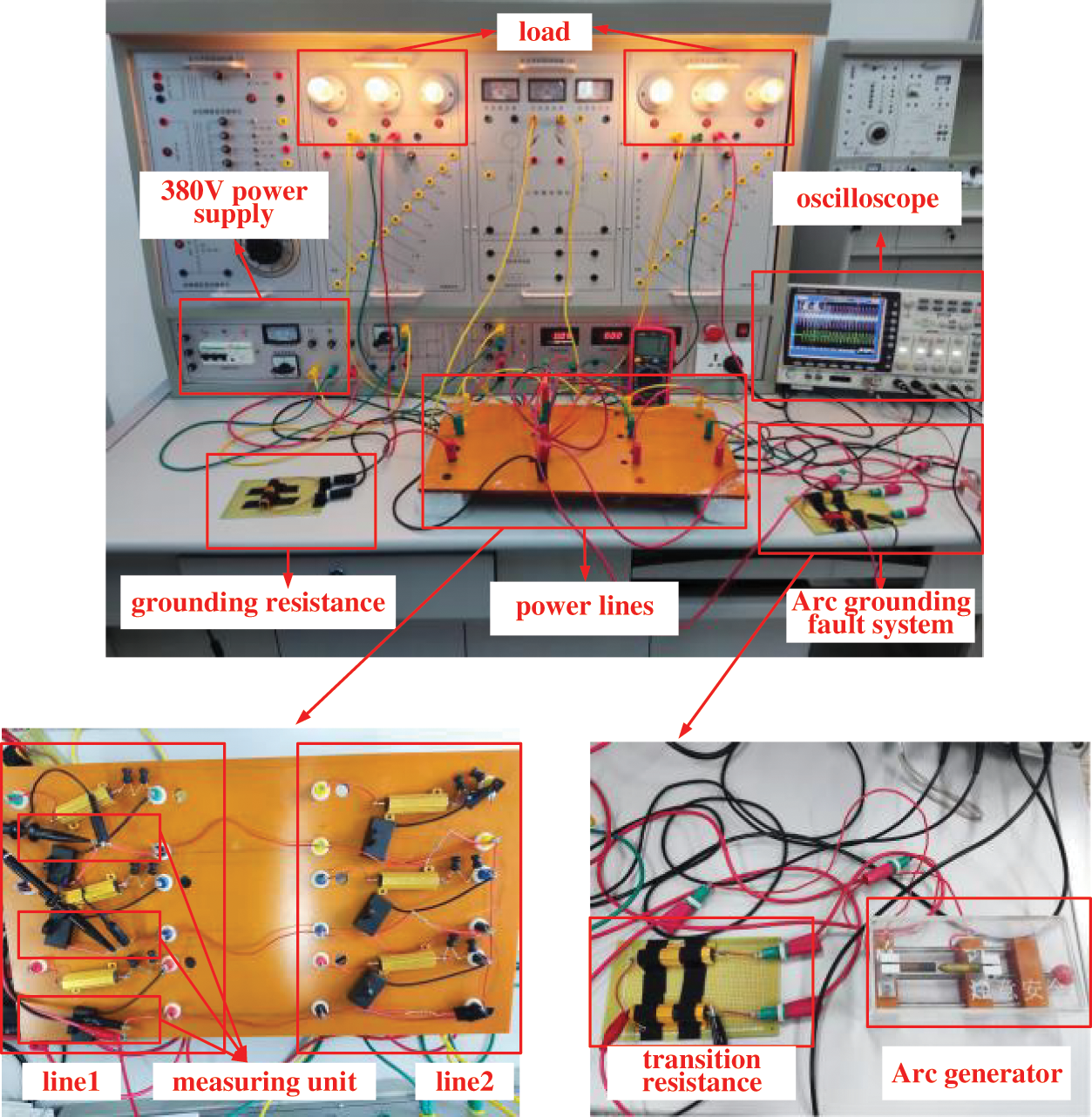
Figure 11: Arc grounding fault test platform

There are two power lines in the experimental network, named line 1 and line 2. The fault is set at phase B of line 2.

The measured signal data are loaded into the procedure of the proposed method. The experimental curve is similar to the results in the aforementioned simulation experiments. The detailed results are shown in Fig. 12.

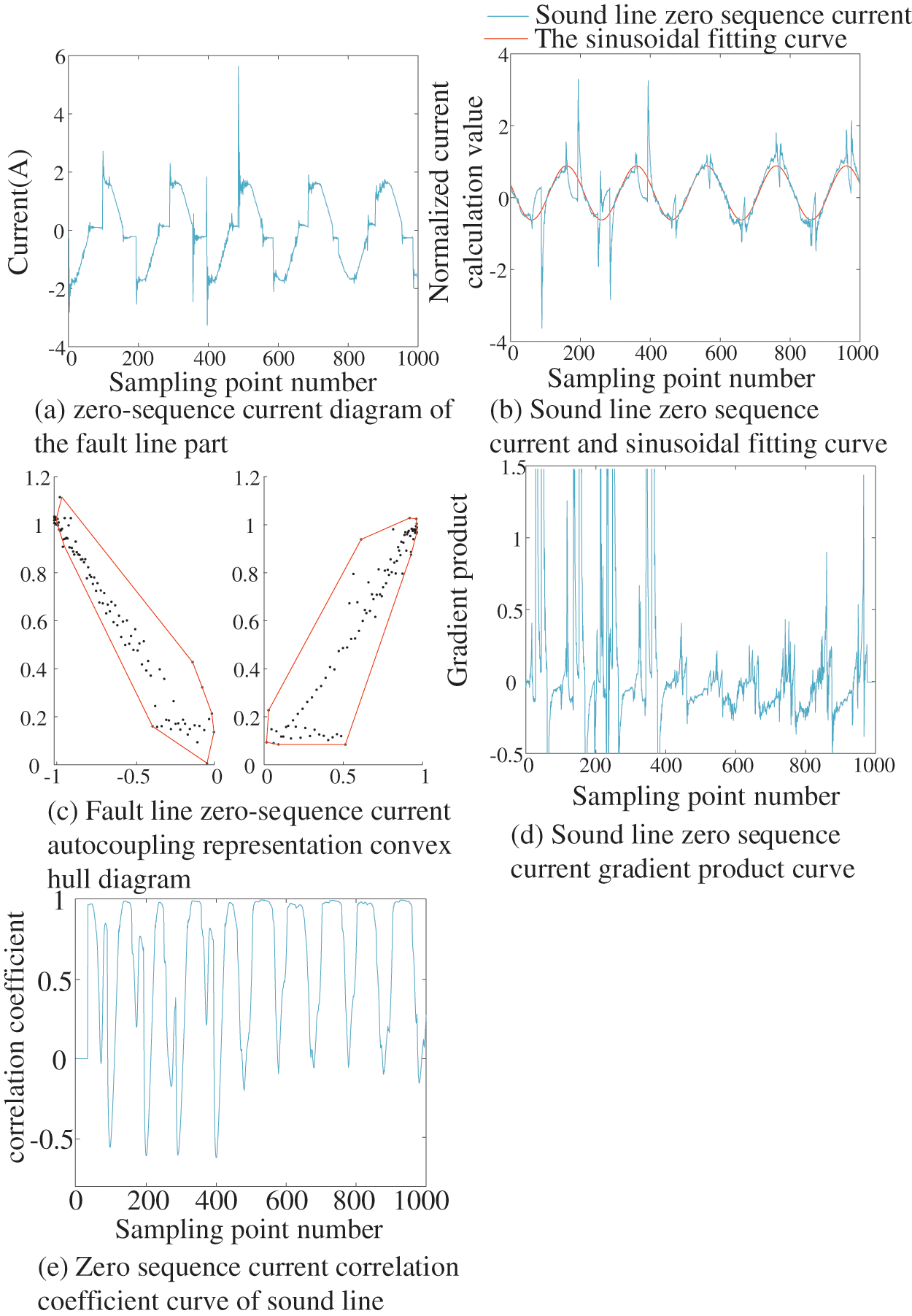
Figure 12: Fault judgment of measured waveform

The basic characteristic parameters obtained from the measured arc grounding fault signal in this example are as follows: convex hull area value left is 0.3429, right is 0.4153, gradient product value is 0.9145, and correlation coefficient value is −0.618. The auxiliary characteristic parameters: variance is 0.285, standard deviation is 0.534.

By substituting the above characteristic parameters into the logistic regression diagnostic model, it can be identified as an arc fault, which proves the effectiveness of the proposed method.

7  Conclusion

(1) The existing arc fault identification methods have some shortcomings in the selection of feature parameters. Most of them only paid attention to the time-frequency domain characteristics of the fault line signal, and ignored the transmission function of the fault characteristics to sound line signals, ignoring the fault characteristics on sound lines. When the arc dissipation power is smaller than 2 × 103 W, the “zero off” feature of the fault line current signal is not obvious, resulting in the accuracy of the identification method using only the fault line signal feature obviously reduced.

(2) It is found that, after the arc grounding fault occurs, there are also rich fault characteristics in the sound line signals. According to the formation mechanism and waveform characteristics, these fault characteristics of sound line signals can be described and characterized by using the gradient product index and correlation coefficient index. The gradient product index of the arc fault is often greater than 0.4, and the correlation coefficient is often much less than 0. These indicators can be used for fault identification, which expands the arc fault identification theory.

(3) Based on the convex hull area index, gradient product index, correlation coefficient index, and logistic regression model, this paper comprehensively extracts the characteristics of fault line signals and sound line signals to achieve arc grounding fault identification. The effectiveness and accuracy of the proposed method are verified by both simulation results and experiment results. The comparative analysis results show that the proposed method has more advantages than the detection method based on kurtosis, harmonic energy, or decomposition features, especially when the zero-off characteristic is not obvious. This method has further improved the accuracy of fault identification, but it needs further research on the identification speed.

Acknowledgement: Thanks to Dr. Zhu Jun, Dr. Du Shaotong, and Dr. Guo Xiangwei for their comments and ideas on this paper, and thanks to the New Energy Power Generation and Intelligent Microgrid Laboratory for their support of the experimental instruments and equipment provided in this paper.

Funding Statement: This work was supported in part by the Natural Science Foundation of Henan Province, and the specific grant number is 232300420301, the initials of author is P. L., the URL to the sponsors’ websites is https://kjt.henan.gov.cn/. And this work was also supported in part by the Fundamental Research Funds for the Universities of Henan Province, and the specific grant numbers is NSFRF220425, the initials of author is P. L., the URL to sponsors’ websites is http://app.hnkjt.gov.cn/web/index.do.

Author Contributions: The authors confirm contribution to the paper as follows: study conception and design: Penghui Liu, Yuxing Dai, Yaning Zhang, Yanzhou Sun; data collection: Yaning Zhang, Yuxing Dai, Yanzhou Sun; analysis and interpretation of results: Penghui Liu, Yaning Zhang; draft manuscript preparation: Penghui Liu, Yaning Zhang. All authors reviewed the results and approved the final version of the manuscript.

Availability of Data and Materials: Data available on request from the authors. The data that support the findings of this study are available from the author, Y. Z., upon reasonable request.

Conflicts of Interest: The authors declare that they have no conflicts of interest to report regarding the present study.

References

1. Li, J., Bi, H. R., Li, C. X., Li, J., Zeng, D. H. et al. (2022). Analysis and calculation method for multiple faults in low-resistance grounded systems with inverter-interfaced distributed generators based on a PQ control strategy. International Journal of Electrical Power & Energy Systems, 138, 107980. https://doi.org/10.1016/j.ijepes.2022.107980 [Google Scholar] [CrossRef]

2. Wang, H., Huang, C. L., Yu, H. N., Zhang, J., Wei, F. (2021). Method for fault location in a low-resistance grounded distribution network based on multi-source information fusion. International Journal of Electrical Power & Energy Systems, 125, 106384. https://doi.org/10.1016/j.ijepes.2020.106384 [Google Scholar] [CrossRef]

3. Li, L., Gao, H. L., Cong, W., Yuan, T. (2023). Location method of single line-to-ground faults in low-resistance grounded distribution networks based on ratio of zero-sequence admittance. International Journal of Electrical Power & Energy Systems, 146, 108777. https://doi.org/10.1016/j.ijepes.2022.108777 [Google Scholar] [CrossRef]

4. Wang, W., Xu, B. Y., Zou, G. F., Liang, D. (2023). Arc fault detection method based on voltage characteristic energy amplitude and phase mapping distribution distances. Electric Power Systems Research, 225, 109866. https://doi.org/10.1016/j.epsr.2023.109866 [Google Scholar] [CrossRef]

5. Meng, Y., Yang, Q., Chen, S. L., Wang, Q., Li, X. W. (2023). Multi-branch AC arc fault detection based on ICEEMDAN and LightGBM algorithm. Electric Power Systems Research, 220, 109286. https://doi.org/10.1016/j.epsr.2023.109286 [Google Scholar] [CrossRef]

6. Khakpour, A., Uhrlandt, D., Methling, R. P., Gortschakow, S., Franke, S. et al. (2017). Impact of temperature changing on voltage and power of an electric arc. Electric Power Systems Research, 143, 73–83. [Google Scholar]

7. Parikh, P., Allcock, D., Luna, R., Vico, J. (2014). A novel approach for Arc-flash detection and mitigation: At the speed of light and sound. IEEE Transactions on Industry Applications, 50(2), 1496–1502. [Google Scholar]

8. Zheng, X., Geng, Y., Zhao, J. (2019). Design of intelligent detection and alarm system for Arc smoke in substation. Electronic Devices, 42(5), 1289–1293 (In Chinese). [Google Scholar]

9. Li, L., Cao, X. Y., Xiao, C. (2012). Intelligent temperature detection based on finite element analysis of low-voltage circuit breaker Arc-extinguishing chamber. World Automation Congress 2012, pp. 331–334. Puerto Vallarta, Mexico. [Google Scholar]

10. Zhou, F. Y., Yin, H., Luo, C., Tong, H. X., Yu, K. et al. (2023). Research on low voltage series Arc fault prediction method based on multidimensional time-frequency domain characteristics. Energy Engineering, 120(9), 1979–1990. [Google Scholar]

11. Park, H. P., Chae, S. (2020). DC series Arc fault detection algorithm for distributed energy resources using arc fault impedance modeling. IEEE Access, 8, 179039–179046. [Google Scholar]

12. Miao, W. C., Wang, Z. F., Wang, F., Lam, K. H., Pong, P. W. T. (2023). Multicharacteristics ARC model and autocorrelation-algorithm based Arc fault detector for DC microgrid. IEEE Transactions on Industrial Electronics, 70(5), 4875–4886. [Google Scholar]

13. Gao, H. X., Wang, Z. Y., Tang, A. X., Han, C. X., Guo, F. Y. et al. (2021). Research on series Arc fault detection and phase selection feature extraction method. IEEE Transactions on Instrumentation and Measurement, 70, 1–8, 2004508. [Google Scholar]

14. Wei, M. J., Zhang, H. X., Shi, F., Xie, W., Zhang, Y. et al. (2019). Identification of arcing grounded fault in distribution network based on harmonic energy and waveform distortion. Automation of Electric Power Systems, 43(16), 148–154 (In Chinese). [Google Scholar]

15. Yoon, H. S., Hong, J. S., Yun, S. Y., Kim, C. H., Lee, Y. W. (2022). Arc modeling and kurtosis detection of fault with arc in power distribution networks. Applied Sciences, 12(6), 2777. [Google Scholar]

16. Lin, H., Wang, Z. L., Guo, Z. H., Zhang, P., Wang, Q. J. et al. (2022). Modeling and identification of a distribution network arc grounding fault considering arc length dynamic variation. Electric Power System Protection and Control, 50(7), 31–39 (In Chinese). [Google Scholar]

17. Liu, Y. L., Guo, F. Y., Li, L., Zheng, J. (2019). Simulation analysis and diagnosis method of series fault Arc in mine power supply system. Journal of China Coal Society, 44(4), 1265–1273 (In Chinese). [Google Scholar]

18. Swarna, K. S. V., Arangarajan, V., Ananth, M. B. J., Kumar, P. V., Veerapandiyan, V. et al. (2022). A KNN based random subspace ensemble classifier for detection and discrimination of high impedance fault in PV integrated power network. Measurement, 187, 110333. https://doi.org/10.1016/j.measurement.2021.110333 [Google Scholar] [CrossRef]

19. Jian, W., Zhou, Z., Li, Z. X., Du, S. X. (2022). A novel fault detection scheme based on mutual k-nearest neighbor method: Application on the industrial processes with outliers. Processes, 10(3), 497. https://doi.org/10.3390/pr10030497 [Google Scholar] [CrossRef]

20. Eslami, M., Jannati, M., Tabatabaei, S. S. (2021). An improved protection strategy based on PCC-SVM algorithm for identification of high impedance arcing fault in smart microgrids in the presence of distributed generation. Measurement, 175, 109149. https://doi.org/10.1016/j.measurement.2021.109149 [Google Scholar] [CrossRef]

21. Miao, W., Xu, Q., Lam, K. H., Pong, P. W. T., Poor, H. V. (2021). DC Arc-fault detection based on empirical mode decomposition of Arc signatures and support vector machine. IEEE Sensors Journal, 21(5), 7024–7033. https://doi.org/10.1109/JSEN.2020.3041737 [Google Scholar] [CrossRef]

22. Qu, N., Zuo, J., Chen, J., Li, Z. (2019). Series Arc fault detection of indoor power distribution system based on LVQ-NN and PSO-SVM. IEEE Access, 7, 184020–184028. https://doi.org/10.1109/ACCESS.2019.2960512 [Google Scholar] [CrossRef]

23. Li, B., Wu, J. (2024). Low-voltage arc fault identification using a hybrid method based on improved salp swarm algorithm–variational mode decomposition– random forest. IEEE Access, 12, 15410–15418. https://doi.org/10.1109/ACCESS.2024.3354177 [Google Scholar] [CrossRef]

24. Jiang, J., Li, W., Wen, Z., Bie, Y., Schwarz, H. et al. (2021). Series Arc fault detection based on random forest and deep neural network. IEEE Sensors Journal, 21(15), 17171–17179. https://doi.org/10.1109/JSEN.2021.3082294 [Google Scholar] [CrossRef]

25. Yin, Z., Wang, L., Yang, S., Gao, Y. (2023). A series Arc fault diagnosis method in DC distribution systems based on multiscale features and random forests. IEEE Sensors Journal, 23(3), 2605–2617. https://doi.org/10.1109/JSEN.2022.3228551 [Google Scholar] [CrossRef]

26. Zhu, Y., Peng, H. (2022). Multiple random forests based intelligent location of single-phase grounding fault in power lines of DFIG-based wind farm. Journal of Modern Power Systems and Clean Energy, 10(5), 1152–1163. https://doi.org/10.35833/MPCE.2021.000590 [Google Scholar] [CrossRef]

27. Gao, J. H., Guo, M. F., Shao, X., Chen, D. Y. (2021). Feature-clustering-based Single-line-to-ground fault section location using auto-encoder and fuzzy C-means clustering in resonant grounding distribution systems. IET Generation, Transmission & Distribution, 15, 938–949. [Google Scholar]

28. Zhang, Q., Ma, W. H., Li, G. L., Ding, J. J., Xie, M. (2022). Fault diagnosis of power grid based on variational mode decomposition and convolutional neural network. Electric Power Systems Research, 208, 107871. https://doi.org/10.1016/j.epsr.2022.107871 [Google Scholar] [CrossRef]

29. Yuan, J. W., Jiao, Z. B. (2022). Faulty feeder detection based on fully convolutional network and fault trust degree estimation in distribution networks. International Journal of Electrical Power & Energy Systems, 141, 108264. https://doi.org/10.1016/j.ijepes.2022.108264 [Google Scholar] [CrossRef]

30. Wang, M. Y., Xu, X. Y., Yan, Z. (2023). Online fault diagnosis of PV array considering label errors based on distributionally robust logistic regression. Renewable Energy, 203, 68–80. [Google Scholar]

31. Wichitaksorn, N., Kang, Y. Y., Zhang, F. Q. (2023). Random feature selection using random subspace logistic regression. Expert Systems with Applications, 217, 119535. [Google Scholar]