
 Submit a Paper
 Propose a Special lssue
 Open Access
ARTICLE

Research on the Icing Diagnosis of Wind Turbine Blades Based on FS–XGBoost–EWMA
1 College of Mechanical Engineering, Inner Mongolia University of Technology, Hohhot, 010051, China
2 Inner Mongolia Key Laboratory of Special Service Intelligent Robotics, Hohhot, 010051, China
3 Institute of Engineering Thermophysics, Chinese Academy of Sciences, Beijing, 100190, China
* Corresponding Authors: Xiaowen Song. Email: ; Qing’an Li. Email:
(This article belongs to the Special Issue: Wind Energy Development and Utilization)
Energy Engineering 2024, 121(7), 1739-1758. https://doi.org/10.32604/ee.2024.048854
Received 20 December 2023; Accepted 19 February 2024; Issue published 11 June 2024
 View Full Text
 Download PDF
Abstract
In winter, wind turbines are susceptible to blade icing, which results in a series of energy losses and safe operation problems. Therefore, blade icing detection has become a top priority. Conventional methods primarily rely on sensor monitoring, which is expensive and has limited applications. Data-driven blade icing detection methods have become feasible with the development of artificial intelligence. However, the data-driven method is plagued by limited training samples and icing samples; therefore, this paper proposes an icing warning strategy based on the combination of feature selection (FS), eXtreme Gradient Boosting (XGBoost) algorithm, and exponentially weighted moving average (EWMA) analysis. In the training phase, FS is performed using correlation analysis to eliminate redundant features, and the XGBoost algorithm is applied to learn the hidden effective information in supervisory control and data acquisition analysis (SCADA) data to build a normal behavior model. In the online monitoring phase, an EWMA analysis is introduced to monitor the abnormal changes in features. A blade icing warning is issued when the monitored features continuously exceed the control limit, and the ambient temperature is below 0°C. This study uses data from three icing-affected wind turbines and one normally operating wind turbine for validation. The experimental results reveal that the strategy can promptly predict the icing trend among wind turbines and stably monitor the normally operating wind turbines.Keywords
Nomenclature
| FS | Feature selection |
| XGBoost | EXtreme gradient boosting |
| EWMA | Exponentially weighted moving average |
| SCADA | Supervisory control and data acquisition |
| RF | Random forest |
| SVM | Support vector machines |
| GBDT | Gradient boosting decision tree |
| RMSE | Root mean square error |
| MAE | Mean absolute error |
| MAPE | Mean absolute percentage error |
| AdaBoost | Adaptive boosting |
| GBDT | Gradient boosting decision tree |
Traditional fossil energy sources are declining, and the greenhouse gases and hazardous substances released by their combustion severely threaten the environment and public health [1]. Renewable energy has garnered widespread attention worldwide to cope with the energy crisis and environmental degradation. Among the numerous renewable energy sources, wind energy is developing rapidly due to its non-polluting nature, abundant resources, and sophisticated technology [2]. High-altitude regions are often selected as ideal sites for wind farms because of their substantial wind energy potential and the high density of cold air [3]. However, these areas are also vulnerable to blade icing, which can reduce power generation, increase component stress, affect the lifespan of turbines [4], and even pose safety hazards due to potential ice detachment from the rotating blades, thus potentially resulting in injuries or fatalities [5]. Currently, several commercial wind turbines utilize the deviations between the actual and theoretical powers of the wind turbine as a criterion to identify blade icing. An alarm is triggered when the deviation exceeds a certain threshold, stopping the wind turbine. However, when the alarm is triggered, a substantial icing area has already formed on the blades [6]. Hence, achieving real-time detection of blade icing in wind turbines and issuing timely warnings to ensure safe operation of wind turbines have become crucial objectives.
The monitoring methods for blade icing faults can be broadly categorized into mechanism-based and data-driven methods [7]. Mechanism-based methods usually develop icing dynamics models and use wind tunnel experiments and numerical simulation techniques to verify results, analyzing the impact of blade icing on the performance of the wind turbine system. These methods also monitor the variations in the physical characteristics of the wind turbine with the help of sensors to determine whether icing is occurring. Muñoz et al. [8] used infrared sensors to investigate blade icing based on the change in emissivity when the blade surface is iced over. Kim et al. [9] employed grating fiber optic sensors to classify ice, water, and air media on wind turbine blades because the shift in Fresnel reflection due to icing produces changes in specific intensity. Wang et al. [10] proposed an improved multi-shot icing computational model to address the challenges posed by periodic changes in the yaw condition field for icing studies. They demonstrated that the model helps analyze complex icing problems via icing wind tunnel experiments and numerical simulations. Manatbayev et al. [11] used a moving reference system to consider the rotation effects on the droplet field and applied the FENSAP–ICE icing calculation software to predict the shape of icing at different angles of attack for a vertical axis wind turbine. Mechanism-based methods exhibit a certain level of accuracy but also have some limitations. First, establishing mechanism models requires high-precision sensors, which are not commonly equipped in most existing wind turbines. Therefore, installing these sensors would incur additional costs. Second, wind turbines operate under complex and variable operating conditions. The accuracy of mechanism models significantly decreases with the change in the operating conditions of the wind turbines, thus restricting their practical utility. The data-driven methods establish the correlations between the condition monitoring data and the wind turbine status by analyzing and mining the data of wind turbine operations, thus achieving the fault diagnosis of the system without knowing the system’s exact analytical model. In recent years, numerous large-scale wind turbines have been equipped with supervisory control and data acquisition (SCADA) systems. With advancements in data mining technology, data-driven methods have become feasible for detecting blade icing in wind turbines [12]. Moreover, SCADA systems comprise a vast amount of monitoring data for various components or subsystems of wind turbines, such as environmental parameters, operational statuses, and control parameters. This comprehensive monitoring capability detects the turbine’s overall condition without requiring additional hardware investment, bolstering the cost-effectiveness of data-driven methods [13]. Bai et al. [14] forwarded a recursive feature elimination and cross-validation method combined with a conduction support vector machine to address high dimensionality and raw data imbalance in data obtained from the SCADA system and effectively tested them on four wind turbines using random forest (RF), support vector machines (SVM), and eXtreme Gradient Boosting (XGBoost) algorithms. Tong et al. [15] combined the support vector data description approach with the traditional fixed weighting strategy, an adaptive weighted kernel extreme learning machine algorithm was developed, and the superiority of the proposed algorithm was verified on two wind turbines. Jia et al. [16] proposed a combined slow feature analysis and SVM strategy to detect wind turbine blade icing faults and revealed that selecting the number of slow features is essential. Liu et al. [17] used the deep autoencoder network to learn multilevel fault features from data obtained from SCADA and implemented the idea of integrated learning to construct an integrated icing detection model by adding classifiers after each hidden layer of the network. Cheng et al. [18] suggested a temporal attention-based convolutional neural network to automatically learn beneficial features from raw time sensor data and detect blade icing.
The number and scale of wind farms are growing rapidly with the development of wind energy. The wind power operation and maintenance model are progressing toward digitalization and intelligence [19]. Data-driven methods exhibit great potential and advantages, but data-driven methods often require an extensive amount of labeled data. Although wind farms daily generate a large number of data, these data often do not have high-quality labels. Moreover, labeling the data is labor-intensive and time-consuming. In addition, normal operations of wind turbines usually lead to an unbalanced dataset. Models trained on unbalanced datasets generate predictions biased toward the majority category and cannot accurately forecast icing faults. Currently, there are two major approaches to data imbalance treatment for the problem of category imbalance. One is based on the data aspect, such as Chen et al. [20], who used undersampling of the normal data to eliminate the effect of imbalance. Xu et al. [21] proposed a similar-functionbased undersampling algorithm to remove redundant normal data, while the synthetic minority over-sampling technique algorithm was applied to generate icing data to achieve data balance. The other strategy is based on algorithms. Peng et al. [22] introduced a focal loss function to replace the traditional cross-entropy loss function, reducing the model prediction bias caused by data imbalanced sets by downweighting simple samples so that the loss function focuses more on training complex samples. Ding et al. [23] combined the ideas of undersampling and ensemble learning by normal data undersampling to yield multiple subsets while assigning icing data to each subset as a way to make the data in each subset balanced and then using temporal convolutional networks to train each subset to obtain multiple classification models. Finally, the predictions of all models are averaged as the final prediction of the sample. However, such methods will likely be affected by hyperparameters or thresholds that are challenging to determine.
To solve this problem, this paper proposes a normal behavior model-based icing warning strategy for wind turbines. The method only learns the normal data from SCADA data and achieves the icing warning of wind turbines based on the discrepancy between the residuals of the model’s predicted and actual values of the normal and icing data, effectively avoiding the problem of data imbalance. Data-driven based methods are categorized into machine learning–based methods and deep learning–based methods. Deep learning dominates the field of fault diagnosis because of its robust feature extraction capabilities, but it requires a large amount of data, which may be lacking in the industry. Machine learning is still widely adopted because of its unique advantages in the presence of insufficient training samples, limited computational resources, and specific learning rules. The XGBoost algorithm, as a classical and efficient integrated learning algorithm, has been widely validated for its excellent performance in several data science competitions [24] and practical applications [25]. Therefore, it is selected in this paper to train the normal behavior model. However, the data recorded by the SCADA system have hundreds of dimensions, which will result in a dimensional catastrophe if all of them are inputted into the model, leading to an overly complex model, overfitting phenomenon. In this regard, to avoid losing the generality, this paper adopts three standard statistical measures, namely Pearson, Spearman, and Kendall, to select the input variables of the normal behavior model. In addition, if the difference in residuals is used to artificially determine whether the blade is iced, it is easily affected by professional knowledge and is highly subjective. This paper introduces the exponentially weighted moving average (EWMA) control chart during the testing phase to monitor the changing trends of the residuals.
This paper’s main contributions can be summarized as follows:
1. The SCADA system documents high-dimensional data, which can cause feature redundancy and affect the accuracy of icing prediction if the original features are used directly. This paper uses Pearson, Spearman, and Kendall methods to select effective features.
2. A machine learning–based fault diagnosis strategy is forwarded to address the problem of the industry’s Insufficient high-quality samples and unbalanced SCADA data. The strategy only uses normal data to train the XGBoost model to avoid the issue of insufficient icing samples.
3. Considering that artificially setting the residual threshold is prone to cause false alarms, EWMA is introduced to analyze the trends of residual change.
The rest of this paper is structured as follows. Section 2 introduces the theoretical background and proposed methods. Section 3 validates the presented method using the data collected from a wind farm in Hubei Province, China, followed by a brief conclusion in Section 4.
2 Feature Selection (FS)–XGBoost–EWMA–Based Icing Warning Model
The wind turbine is an electrical, mechanical device that harvests energy from the wind to generate power. Ice on the blades results in uneven quality, affecting the aerodynamic characteristics and reducing the output power at the same wind speed. Therefore, this paper selects the 60 s average power in the dataset as the monitoring feature. In order to select appropriate modeling variables, this paper uses the Pearson, Spearman, and Kendall methods to calculate the correlation coefficient between 60 s average active power and other variables to determine the input of the normal behavior model.
For the input variable
where n represents the number of samples. The
The Spearman’s rank correlation coefficient formula is expressed as follows:
where
The formula for the Kendall rank correlation coefficient is described as follows:
The Kendall rank correlation coefficient measures the dependent correlation between two variables, with
Table 1 presents the relationship between the correlation values and strengths used in this paper.

To ensure the effectiveness of the features, this paper deletes the weakly correlated and very weakly correlated features. It selects the features whose absolute values of the three correlation coefficients are all greater than 0.4 as the inputs of the early warning model for wind turbine icing.
The XGBoost algorithm is an integrated algorithm based on gradient boosting decision tree (GBDT) model optimization proposed by Chen et al. [26]. Its basic idea is to fit the residuals of previous training by continuously training a new decision tree model and accumulating the results of all trees as the final prediction [27].
Suppose a dataset of n samples and m features is given:
Here,
XGBoost contains K trees; therefore, the prediction result for a sample can be expressed as follows:
where
The objective function is defined as follows:
where
A greedy algorithm is used during XGBoost training to add a new regression decision tree to the existing model one at a time [28]. XGBoost gradually improves the model’s prediction ability by continuously adding new regression decision trees to fit the modeling residuals of the current model. Assuming that the predicted sample value
where
The objective function can be expressed as follows:
where at the
XGBoost performs a second-order Taylor expansion of the objective function to provide a more accurate approximation of the objective function. After deleting the constant term, the objective function is expressed as follows:
where
SCADA data have the characteristics of complex sources, information coupling, and strong time variability; these changes are nonlinear. Taylor’s formula is a commonly used mathematical tool for approximating nonlinear functions. XGBoost’s quadratic Taylor expansion of the loss function can provide a more accurate approximation of the objective function, better capturing the nonlinear relationship in the SCADA data.
Furthermore, by transforming the objective function into an accumulation of leaf nodes and defining the
The set of samples on each leaf node
where
By calculating information gain on leaf nodes, the XGBoost model can distinguish practical features from multi-dimensional SCADA data and select nodes with the most extensive information gain to split, thereby building a highly accurate and robust normal behavior model. The calculation of information gain in XGBoost is presented as follows:
where
2.3 Exponential Weighted Average of Movement
Because the normal behavior model is trained based on the normal SCADA data, the residuals between the model’s predicted and actual values for normal samples are relatively small. However, the normal behavior model does not learn from icing samples; the residuals between the model’s predicted and actual values for icing samples are relatively large. Therefore, in this paper, the residuals between the model predicted values and the actual values of the samples are used to achieve the early warning of icing in wind turbines. The residual difference formula is expressed as follows:
where
SCADA data are time series data, and EWMA is a commonly used time series smoothing method. It performs a weighted average of the time series, assigning higher weights to the most recent observations and lower weights to earlier observations. This enhances its ability to capture the trend of the series and the tiny fluctuations or changes. Meanwhile, the operating conditions of wind turbines are very complex and variable, and the SCADA data are highly variable [29]. Therefore, this paper uses EWMA to analyze the residual series to detect abnormalities in time.
The formula for calculating the value of EWMA is shown as follows:
where
Due to blade icing, the actual power of the wind turbine is reduced, and the large prediction of the monitored values by the obtained warning model trained under normal conditions results in negative residuals; therefore, the lower limit of the EWMA control chart is selected in this paper to generate the warnings for wind turbine icing.
where
2.4 Early Warning Strategy of Wind Turbine Based on FS–XGBoost–EWMA
Fig. 1 shows the wind turbine early warning strategy based on the FS–XGBoost–EWMA system proposed in this paper. It is divided into two parts: offline training and online monitoring.
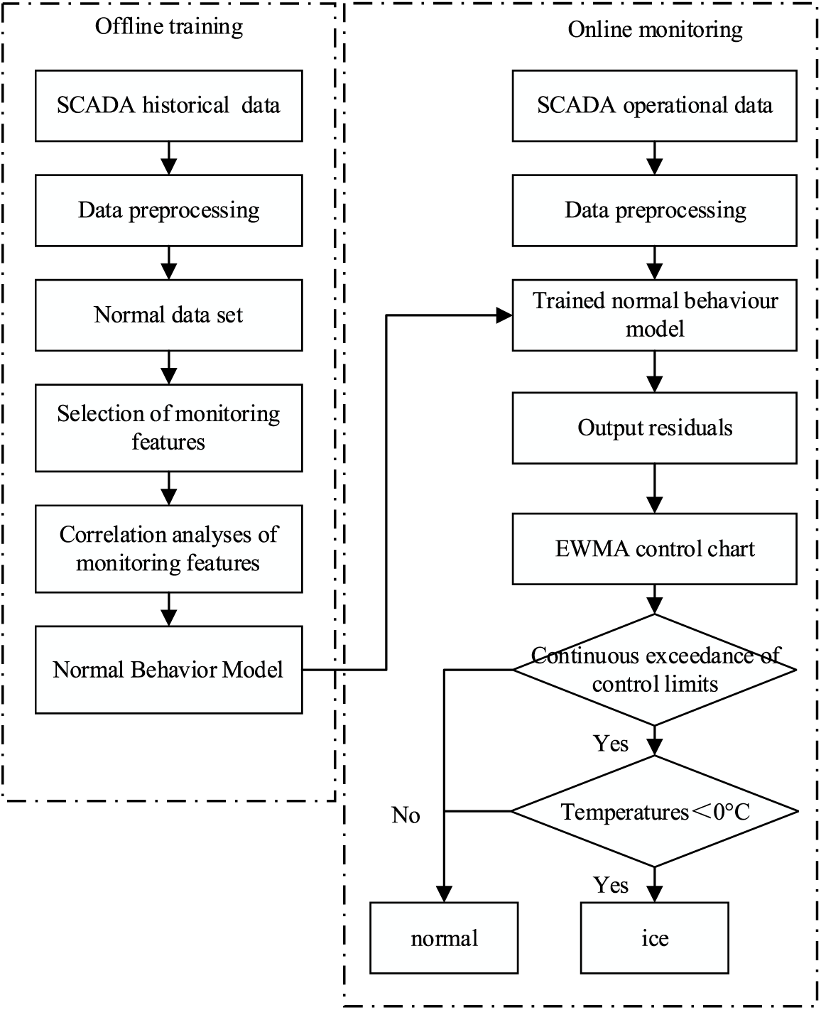
Figure 1: Wind turbine icing warning strategy
Offline training: due to the complex and variable operating conditions of wind turbines, the original dataset contains a huge amount of bad data with zero generator torque, active power less than or equal to zero, and wind speed less than the cut-in or greater than the cut-out wind speed. The data for the wind turbine mentioned above shutdown period are deleted to obtain the training set for normal operation. Meanwhile, after severe icing, the SCADA data are deleted. Next, the correlation analysis is performed on the 60 s average active power. This article selects features whose absolute values of three correlation coefficients, namely, Pearson, Spearman, and Kendall, are all greater than 0.4 to train the XGBoost normal behavior model.
Online monitoring: to simulate the online monitoring phase, data from the day of the wind turbine icing shutdown and normal data from the previous day are selected for testing. First, the same preprocessing is performed on the test set, and the data within 2 min before the wind turbine shutdown is excluded. Next, the features related to the monitoring variables are input into the normal behavior model obtained in the training phase to obtain the predicted value of the 60 s average active power under the normal operation condition; furthermore, the residual difference between the predicted value and the actual value of the 60 s average active power is computed, and the residual is subjected to the EWMA analysis. If the temperature is less than 0°C and exceeds the control limit for ten consecutive times, the wind turbine is considered to be in icing condition; otherwise, the wind turbine is considered as normal.
3 Calculation Example of the Validation Analysis
3.1 Introduction to the Datasets
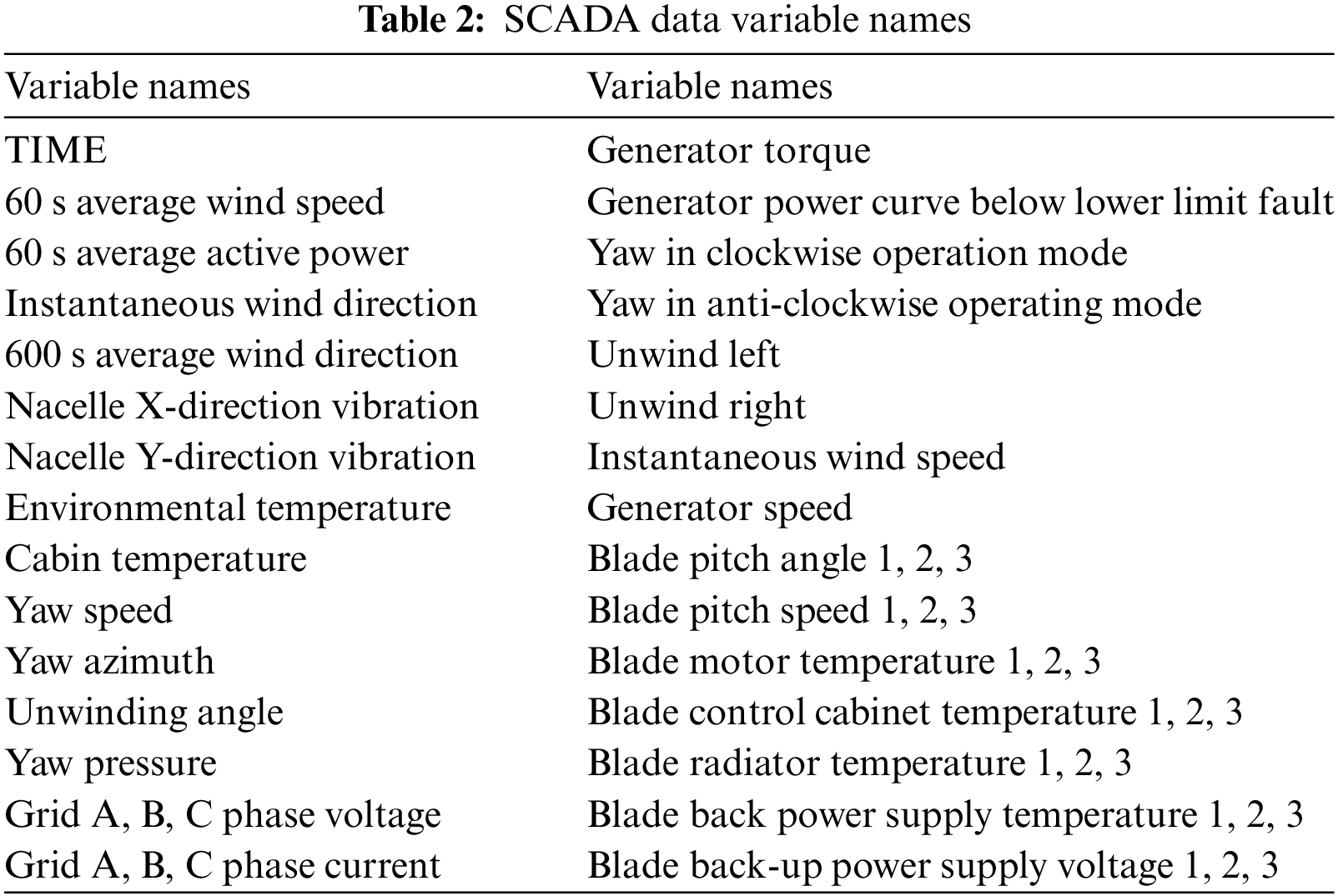
In this paper, the SCADA data of three icing wind turbines and one normal wind turbine from a wind farm in the Hubei Province of China were selected for blade icing warning validation and analysis. The rated power of the wind turbines was 2.5 MW, the cut-in wind speed was 3 m/s, the cut-out wind speed was 25 m/s, the rated wind speed was 12.5 m/s, and the sampling period of the SCADA system was 1 min. The datasets recorded the operating parameters of the wind turbines and the environmental parameters (Table 2). Table 3 presents the operating status of the four wind turbines.
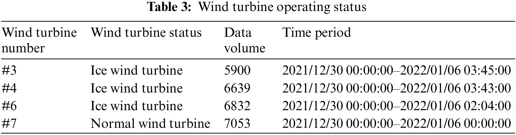
The original data contains a large amount of bad data. In this paper, all of them and the data two minutes before the wind turbine shutdown are deleted to obtain the data shown in Table 3. The time period of icing wind turbine extends from normal operation to wind turbine icing shutdown. The icing wind turbine takes the #3 wind turbine as an example. This paper selects the data from December 30, 2021–January 04, 2022, for model training and validation. Notably, the data on the day of icing and the previous day are selected to simulate online prediction. The data from December 30, 2021–January 04, 2022, of the normal wind turbine in this paper are selected for model training and validation, and the data on January 05, 2022, are simulated for online testing.
To assess the model’s performance, this paper employs the root mean square error (RMSE), mean absolute error (MAE), and mean absolute percentage error (MAPE) as evaluation measures:
3.3 Wind Turbine Warning under Icing Condition
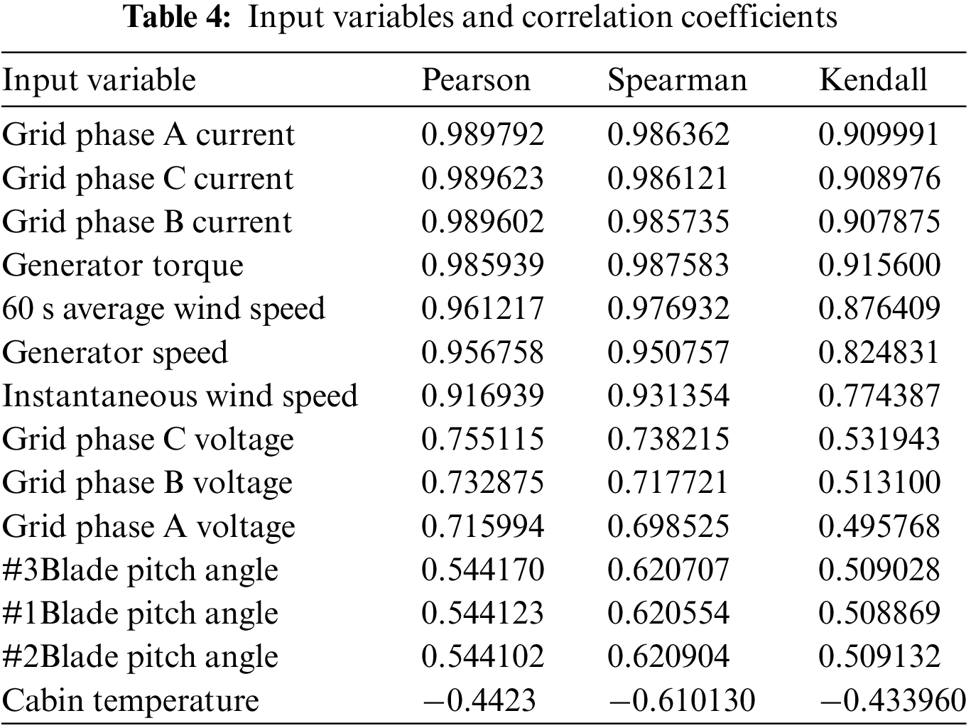
To establish an effective icing warning model for wind turbines, this paper selected the data from December 30 2021, to January 04, 2022, for analysis and divides it into a training set and a verification set in a ratio of 8:2. First, the Pearson, Spearman, and Kendall correlation coefficient methods are used to calculate the correlation coefficient between the 60 s average active power and other variables. In this paper, the variables whose absolute values of three correlation coefficients are all greater than 0.4 are taken as the inputs of the normal behavior model. The variable is deleted if any correlation coefficient is less than 0.4. Table 4 shows the correlation coefficient values between the input variables and the 60 s average active power.
To verify the prediction performance of the XGBoost algorithm, this paper selects RF, SVM, AdaBoost, and GBDT algorithms to compare, learn the information hidden in SCADA data on the training set, and evaluate it on the verification set to select the optimal wind turbine icing warning normal behavior model. Table 5 compares the prediction results of different methods.
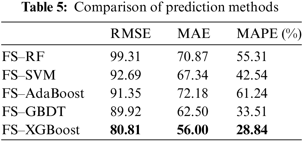
The comparison results in Table 5 reveal that the RMES, MAE, and MAPE of the XGBoost algorithm are better than that of RF, SVM, AdaBoost, and GBDT algorithms. Compared with the worst RF algorithm, the three error indicators are improved by 18.63%, 20.98%, and 47.86%, respectively. Compared with the GBDT algorithm, the three error indicators are improved by 10.13%, 10.4%, and 13.94%, respectively. The quadratic Taylor expansion of the loss function by XGBoost can better learn the effective information characterizing wind turbine icing in SCADA data.
Sensitivity analysis evaluates the impact on the output results by changing the model’s input parameters. The hyperparameters such as n_estimators, learning_rate, and max_depth play a crucial role in the performance of the XGBoost algorithm. This paper conducts sensitivity analysis on the three parameters mentioned above to evaluate the effects of different hyperparameters on model performance. Among them, n_estimators represents the number of base learners in XGBoost. The greater the number, the stronger the learning ability of the model, but the model is also more accessible to overfit. Considering the size of the dataset, this article sets the number of n_estimators to 50, 100, and 150 for analysis; the learning_rate parameter represents the learning rate, and the value range is usually between [0.01,0.3]. This article sets the learning_rate to 0.01, 0.1, 0.3 for analysis. max_depth controls the maximum depth of the tree in the model, and the value usually ranges between [3,10]. This article sets max_depth to 3, 6, and 9 for analysis. Finally, the analysis results are shown in Tables 6–8.
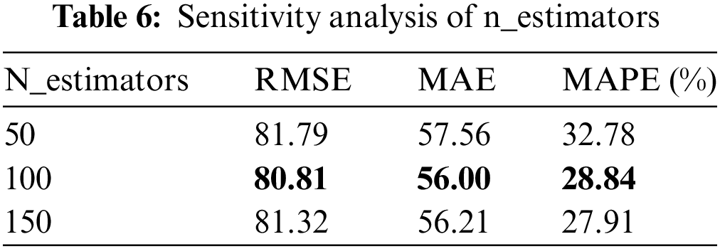
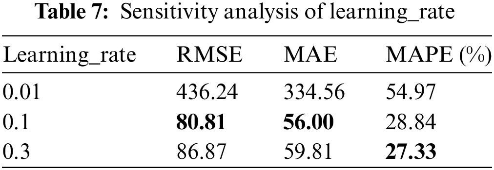

Table 6 shows that when n_estimators is 100, all three model indicators perform best. Table 7 shows that when the learning_rate is 0.1, RMSE and MAE are better than other learning_rates, but MAPE is smaller than learning_rate of 0.3. Considering that when the learning_rate is 0.1, the model’s overall performance is better and 0.1 is selected as the optimal learning rate. Max_depth is similar to learning_rate, and the larger the max_depth value, the more complex the model and the higher the requirements for computing resources and memory space; therefore, max_depth is selected as 3. The n_estimators, learning_rate, and max_depth of the optimal normal behavior model in this paper are set to 100, 0.1, and 3, respectively. Fig. 2 depicts the loss function curve of the normal behavior model.
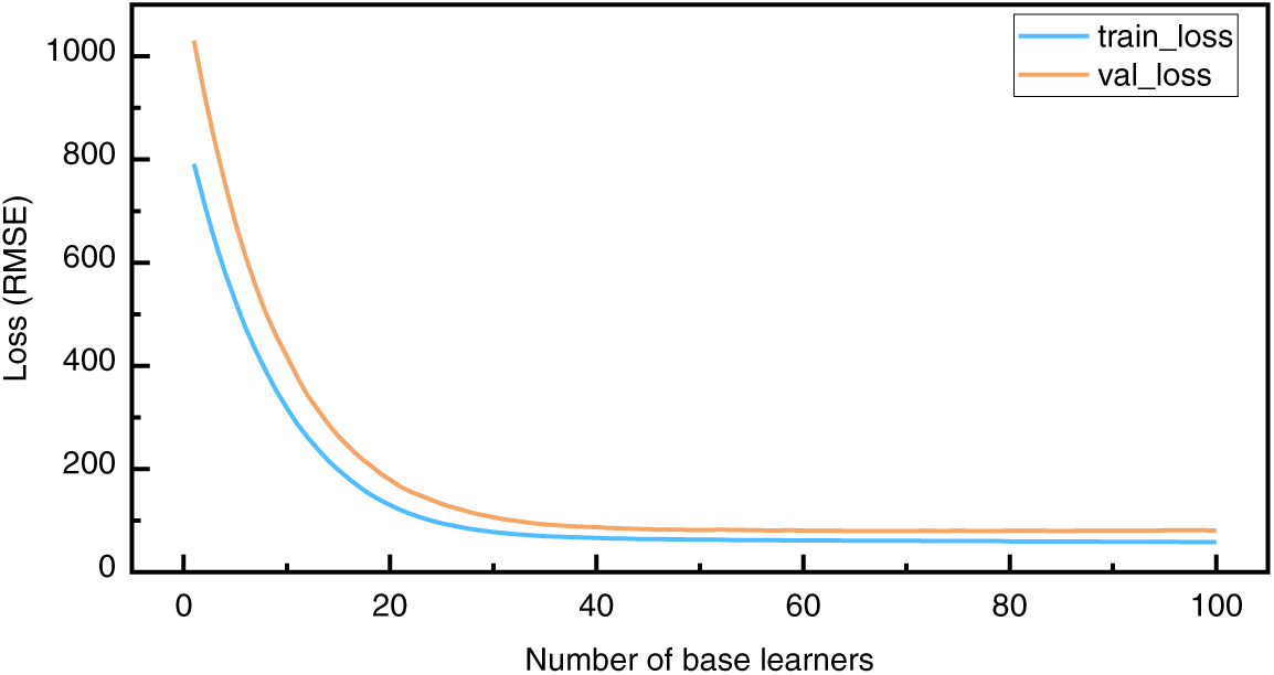
Figure 2: Loss function iteration curve
Fig. 2 shows that at the beginning of training, the model’s loss value on the training set and verification set dropped significantly, indicating that the learning rate was appropriate. At 40 iterations, the loss curve became stable. In the later stage of training, the model reached a state of convergence. The model can fit the training data well and perform better on the validation set. The normal behavior model obtained through training is highly robust and highly generalizable.
To verify the effectiveness of the icing warning strategy for wind turbines proposed in this paper, the optimal normal behavior model was selected to verify the data on the day of wind turbine shutdown due to icing and the day before (2022-01-05 00:00:00–2022-01-06 03:45:00). The actual and predicted values of the 60 s average active power are shown in Fig. 3, where the red curve is the 60 s average active power. The blue curve is the model’s predicted value.
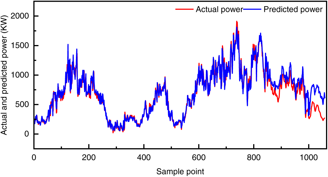
Figure 3: Comparison of model actual and predicted values of #3 wind turbine
Fig. 3 shows that the normal behavior model has a good prediction of the normal data of the test set. Before the icing and shutdown of the wind turbines, there is an apparent deviation between the predicted value and the actual value of the model, which can achieve the effect of initially judging the icing of the wind turbines.
However, depending only on the residuals between the predicted and actual values of the normal behavior model to determine the icing of wind turbines makes it easy to introduce human error. Hence, this paper adopts the EWMA method to analyze the prediction residuals of the model.
Fig. 4 depicts the residual analysis results, wherein the red curve is the threshold curve, the purple curve is the sample points that have not exceeded the control limit, and the green curve is the sample points that have exceeded the control limit. Fig. 4 demonstrates the 60 s average active power EWMA curve appears to exceed the control limit at the 178th point and near the 215th point. According to the judgment criterion shown in Fig. 1, the wind turbines are considered to be in normal working condition because there is no consecutive exceeding of the control limit. However, continuous exceeding of the control limits occurred at the 840th sample point and lasted almost until the wind turbine blade shut down due to icing. According to the temperature variation curve of the test set in Fig. 5, the environment temperature was below zero; hence, the wind turbines were judged to be in an icing condition at the 849th sample point, and a warning was issued. This is 209 sample points (3.5 h) earlier than the downtime recorded in the wind turbine operation log.
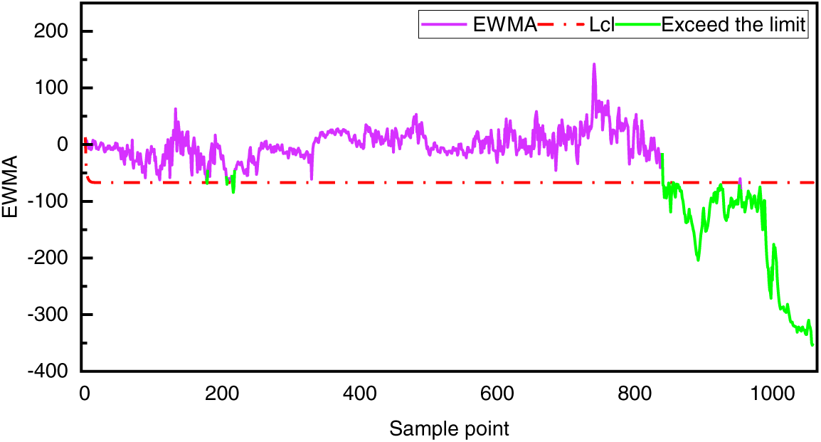
Figure 4: EWMA residual of #3 wind turbines
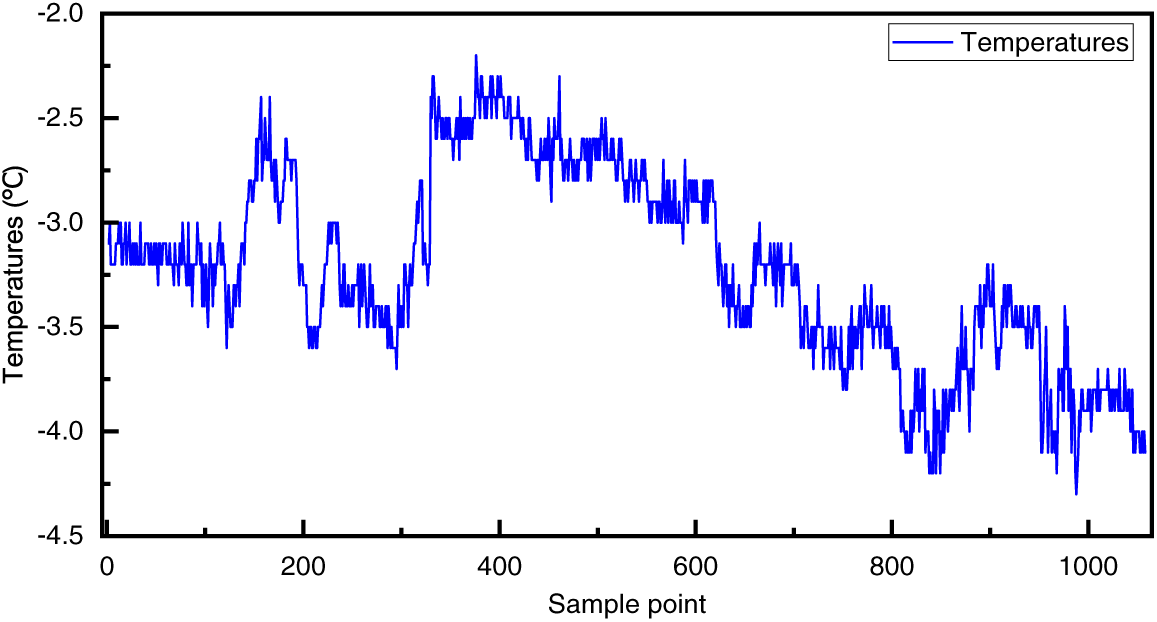
Figure 5: Temperature change curve of #3 wind turbine
Ablation studies refer to the targeted removal or modification of a part of the model, and the effect of that part on the model as a whole is investigated by controlling the variable style. To verify the effectiveness of FS, this paper uses the XGBoost algorithm to perform an ablative analysis of FS, and the experimental results are shown in Fig. 6.
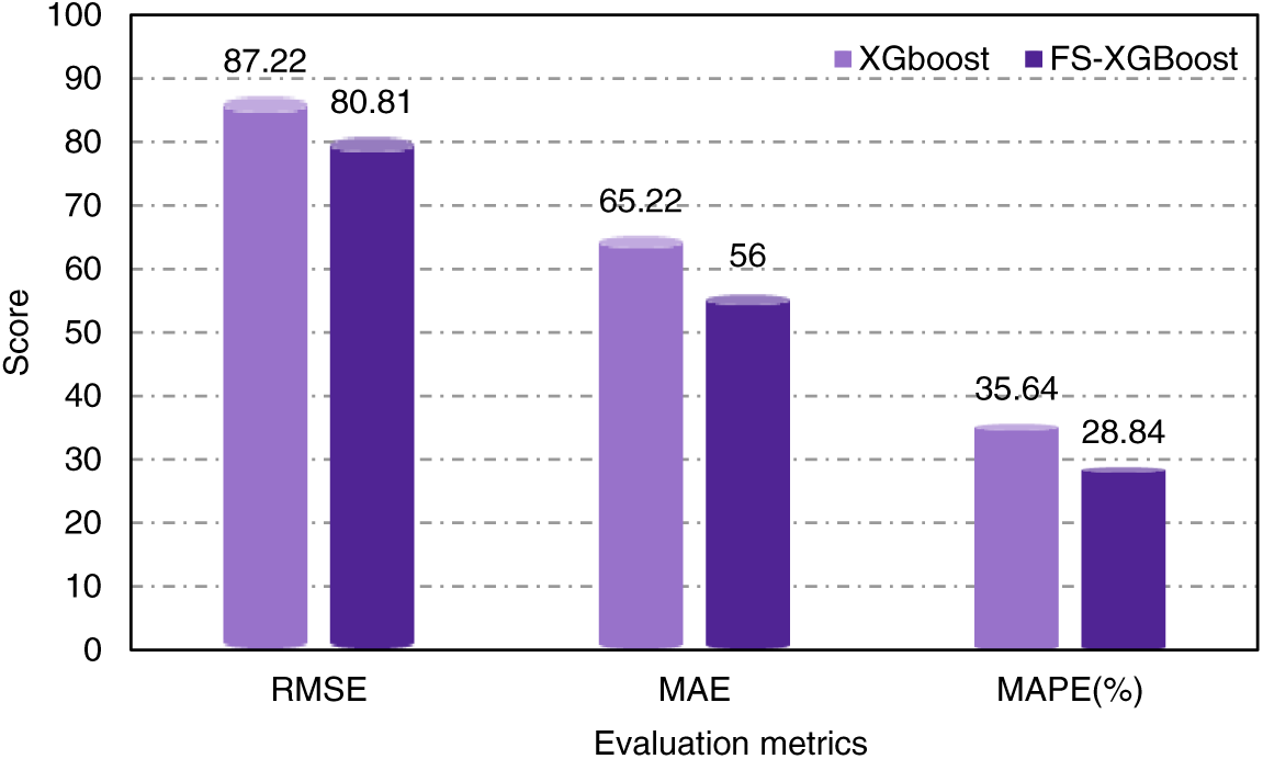
Figure 6: Ablative analysis of feature selection
Fig. 6 demonstrates that FS–XGBoost improves RMSE, MAE, and MAPE by 7.35%, 14.14%, and 19.08%, respectively, compared with XGBoost, indicating that reasonable FS helps improve the prediction performance of the model. Subsequently, this paper compares the effect of XGBoost and FS–XGBoost icing warnings on the test set (Fig. 7).
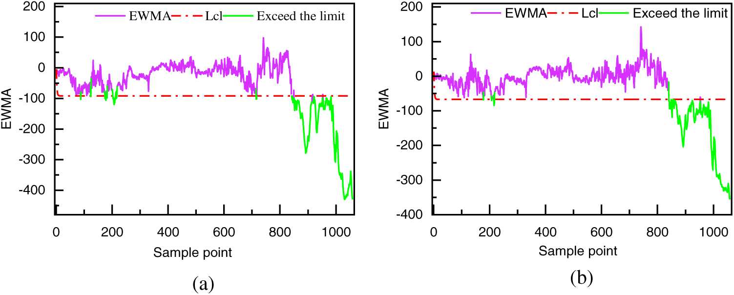
Figure 7: Feature selection ablativity analysis
Fig. 7a shows the warning effect of XGBoost on the test set, and Fig. 7b depicts the warning effect of FS–XGBoost on the test set. XGBoost has more sample points beyond the control limit in the normal part of the test set compared to FS–XGBoost, indicating that FS–XGBoost fits the normal samples better and has a lower probability of false alarms in the future.
To further validate the generalization performance of the icing warning strategy, the strategy proposed in this paper is migrated to #4 and #6 wind turbines for validation, and the predicted values of the normal behavioral model on #4 and #6 wind turbines are depicted in Fig. 8.
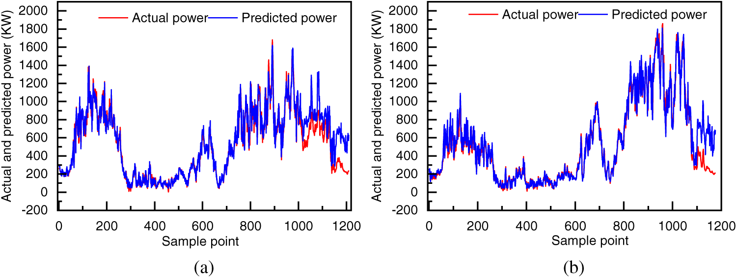
Figure 8: Actual and predicted power of #4 and #6 wind turbines
Figs. 8a and 8b show the actual and predicted values of the power of the #4 wind turbine and #6 wind turbine, respectively. Fig. 8 reveals that in the normal part of the test set, the predicted and actual values of the proposed model are highly fitted. In the place close to the severe icing of the wind turbines, there is a deviation between the model’s predicted and actual values, which can better reflect the differences between the residuals of the predictions of the normal samples and those of the icing samples.
The residuals of the two wind turbines are further analyzed using EWMA (Fig. 9).
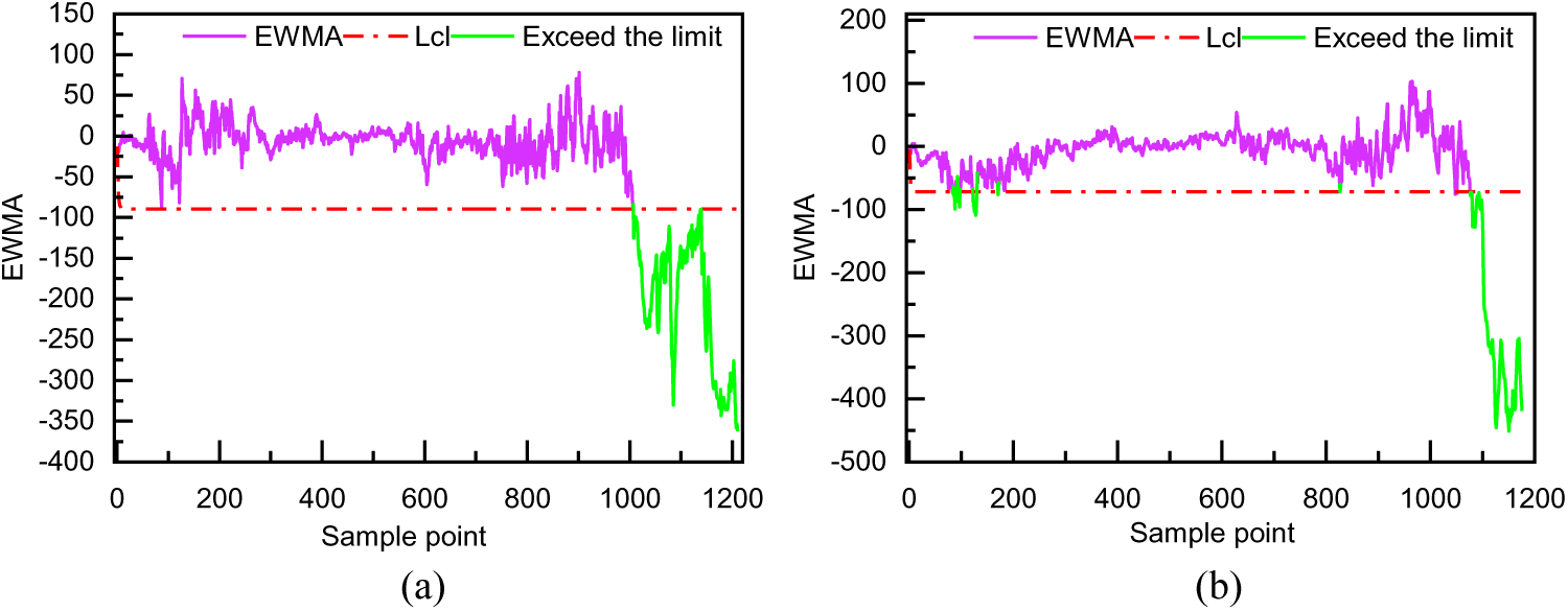
Figure 9: EWMA residual test of #4 and #6 wind turbines
The results of the EWMA analysis are shown in Fig. 9 of the #4 wind turbine and #6 wind turbine. Combined with the judgment criterion proposed in Fig. 1 and the temperature variation curve in Fig. 10, the method proposed in this paper achieves good performance on both #4 and #6 wind turbines. It can respond promptly to the operating status of the wind turbines. Compared with the downtime recorded in the wind turbine’s operation log, the proposed method’s warning time is advanced by 3 and 1.5 h, respectively. Although the normal part of #6 wind turbine exceeds the threshold curve at individual points, it does not exceed the control limit for ten consecutive minutes; thus, it can still provide a reliable assurance for the safe operation of the wind turbine.
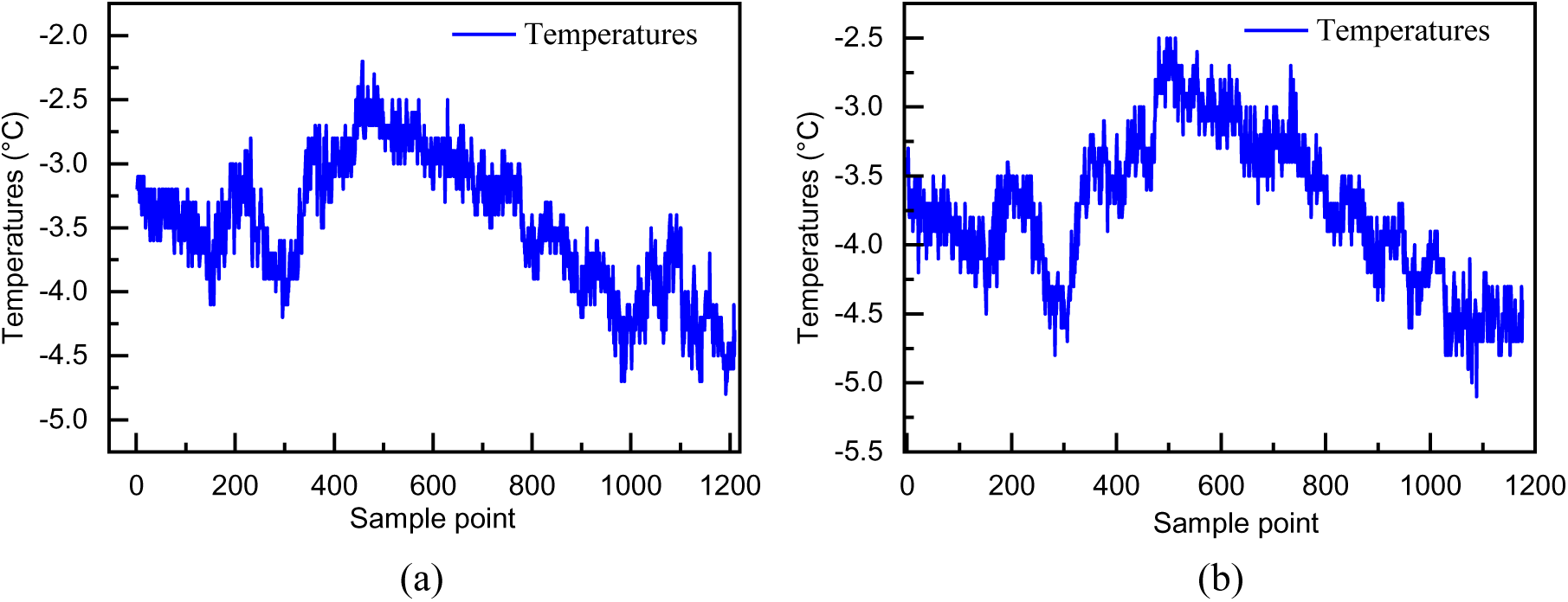
Figure 10: Environment temperature change curve of #4 and #6 wind turbines
3.4 Condition Monitoring of Wind Turbine under Normal Condition
To prevent the possibility of false alarms in the proposed method, this paper further verifies the effectiveness of the proposed method on a normal wind turbine. Fig. 11 illustrates the test results of a normal wind turbine, the prediction and actual value of the 60 s average active power, the EWMA control chart, and the temperature change of the test set. Fig. 11 shows that the actual value of the 60 s average active power and the model’s predicted value fit well. Most EWMA values are within the lcl threshold, despite individual sample points exceeding the threshold limit. According to the judgment criteria, there is no continuous exceeding of the phenomenon, which will not issue an alarm, proving the effectiveness of the proposed method for monitoring the status of normal wind turbines and avoiding false alarms.
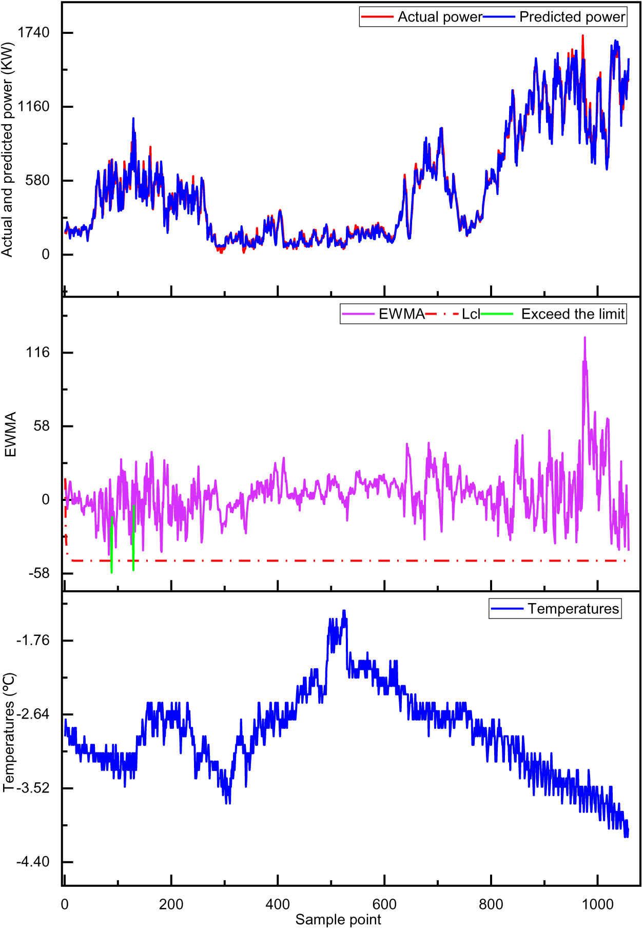
Figure 11: Normal wind turbine condition monitoring effect
To address the issue of limited training samples and insufficient icing samples in data-driven methods, this paper proposes an FS–XGBoost–EWMA–based icing warning strategy for wind turbines. The strategy adopts XGBoost to establish a normal behavior model for wind turbine icing warnings and takes the discrepancy between the residuals of the model’s predicted and the actual values as the warning indicator. Next, it selects Pearson, Spearman, and Kendall methods to determine the model inputs and introduces the EWMA method to analyze the predicted residual in real time during the online monitoring stage. If the monitoring data exceeded the control limits for ten consecutive times, and the temperature was below 0°C the wind turbines were considered to be iced.
The main conclusions are presented as follows:
1. Compared with RF, SVM, AdaBoost, and GBDT algorithms, the XGBoost algorithm has better generalization ability and is more suitable for the high-dimensional and nonlinear characteristics of SCADA data.
2. Compared with XGBoost, FC–XGBoost has higher prediction accuracy, and the use of Pearson, Spearman, and Kendall helps improve the model’s performance.
3. Introducing EWMA to analyze the prediction residuals of the model can provide robust thresholds.
The proposed strategy is validated on three icing wind turbines and one normal wind turbine. It can predict the icing trend of wind turbines in time and monitor the normal operation of wind turbines stably. However, this paper still has the following shortcomings:
1) This paper only uses seven days of validation data, which is relatively less for the data-driven approach. In the future, it is necessary to collect more wind turbine data samples to validate the method proposed in this paper more comprehensively.
2) A wind turbine is a multi-coupled complex system, and this paper only considers monitoring the 60 s average active power. In the future, it is necessary to consider more monitoring features to comprehensively monitor the operating status of wind turbines with multiple parameters.
Acknowledgement: None.
Funding Statement: This research was funded by the Basic Research Funds for Universities in Inner Mongolia Autonomous Region (No. JY20220272), the Scientific Research Program of Higher Education in Inner Mongolia Autonomous Region (No. NJZZ23080), the Natural Science Foundation of Inner Mongolia (No. 2023LHMS05054), and the National Natural Science Foundation of China (No. 52176212). We are also very grateful to the Program for Innovative Research Team in Universities of Inner Mongolia Autonomous Region (No. NMGIRT2213) The Central Guidance for Local Scientific and Technological Development Funding Projects (No. 2022ZY0113).
Author Contributions: Jicai Guo: Writing, Original draft, Conceptualization, Methodology. Xiaowen Song: Conceptualization, Writing–review & editing, Supervision, Funding acquisition. Chang Liu: Data curation, Visualization. Yanfeng Zhang: Investigation, Formal analysis. Shijie Guo: Investigation, Data curation. Jianxin Wu: Supervision, Validation. Chang Cai: Supervision, Methodology. Qing’an Li: Project administration, Supervision, Funding acquisition. All authors reviewed the results and approved the final version of the manuscript.
Availability of Data and Materials: The data used in this study are confidential at the request of the wind farm operators.
Conflicts of Interest: The authors declare that they have no conflicts of interest to report regarding the present study.
References
1. Lei, X., Alharthi, M., Ahmad, I., Aziz, B., Abdin, Z. (2020). Importance of internationalrelations for the promotion of renewable energy, preservation of natural resources andenvironment: Empirics from SEA nations. Renewable Energy, 196, 1250–1257. [Google Scholar]
2. Zhang, S., Wei, J., Chen, X., Zhao, Y. (2020). China in global wind power development: Role, status and impact. Renewable and Sustainable Energy Reviews, 127, 109881. https://doi.org/10.1016/j.rser.2020.109881 [Google Scholar] [CrossRef]
3. Ali, Q., Kim, M. (2021). Design and performance analysis of an airborne wind turbine for high-altitude energy harvesting. Energy, 230, 120829. https://doi.org/10.1016/j.energy.2021.120829 [Google Scholar] [CrossRef]
4. Lehtomäki, V., Rissanen, S., Wadham-Gagnon, M., Sandel, K., Moser, W. et al. (2016). Fatigue loads of iced turbines: Two case studies. Journal of Wind Engineering and Industrial Aerodynamics, 158, 37–50. https://doi.org/10.1016/j.jweia.2016.09.002 [Google Scholar] [CrossRef]
5. Jia, Y., Cheng, B., Li, X., Zhang, H., Dong, Y. (2020). Research on effect of icing degree on performance of NACA4412 airfoil wind turbine. Energy Engineering, 117(6), 413–427. https://doi.org/10.32604/EE.2020.012019 [Google Scholar] [CrossRef]
6. Tao, T., Liu, Y., Qiao, Y., Gao, L., Lu, J. et al. (2021). Wind turbine blade icing diagnosis using hybrid features and stacked-XGBoost algorithm. Renewable Energy, 180, 1004–1013. https://doi.org/10.1016/j.renene.2021.09.008 [Google Scholar] [CrossRef]
7. Tian, W. (2022). Icing detection of wind turbine blades based on machine learning (Master Thesis). Tianjin University of Technology, China. [Google Scholar]
8. Muñoz, C. Q. G., Márquez, F. P. G., Tomás, J. M. S. (2016). Ice detection using thermal infrared radiometry on wind turbine blades. Measurement, 93, 157–163. https://doi.org/10.1016/j.measurement.2016.06.064 [Google Scholar] [CrossRef]
9. Kim, D. -G., Sampath, U., Kim, H., Song, M. (2017). A fiber-optic ice detection system for large-scale wind turbine blades. Proceedings of the Optical Modeling and Performance Predictions IX, pp. 52–57. San Diego, USA. [Google Scholar]
10. Wang, Q., Yi, X., Liu, Y., Ren, J., Li, W. et al. (2020). Simulation and analysis of wind turbine ice accretion under yaw condition via an improved multi-shot icing computational model. Renewable Energy, 162, 1854–1873. https://doi.org/10.1016/j.renene.2020.09.107 [Google Scholar] [CrossRef]
11. Manatbayev, R., Baizhuma, Z., Bolegenova, S., Georgiev, A. (2021). Numerical simulations on static vertical axis wind turbine blade icing. Renewable Energy, 170, 997–1007. https://doi.org/10.1016/j.renene.2021.02.023 [Google Scholar] [CrossRef]
12. Tautz-Weinert, J., Watson, S. J. (2016). Using SCADA data for wind turbine condition monitoring—A review. IET Renewable Power Generation, 11(4), 382–394. [Google Scholar]
13. Zhang, L., Liu, K., Wang, Y., Omariba, Z. B. (2018). Ice detection model of wind turbine blades based on random forest classifier. Energies, 11(10), 2548. https://doi.org/10.3390/en11102548 [Google Scholar] [CrossRef]
14. Bai, X., Tao, T., Gao, L., Tao, C., Liu, Y. (2023). Wind turbine blade icing diagnosis using RFECV-TSVM pseudo-sample processing. Renewable Energy, 211, 412–419. https://doi.org/10.1016/j.renene.2023.04.107 [Google Scholar] [CrossRef]
15. Tong, R., Li, P., Lang, X., Ling, J., Cao, M. (2021). A novel adaptive weighted kernel extreme learning machine algorithm and its application in wind turbine blade icing fault detection. Measurement, 185, 110009. https://doi.org/10.1016/j.measurement.2021.110009 [Google Scholar] [CrossRef]
16. Jia, P., Chen, G. (2020). Wind power icing fault diagnosis based on slow feature analysis and support vector machines. Proceedings of the 2020 10th International Conference on Power and Energy Systems (ICPES), pp. 398–403. Chengdu, China. [Google Scholar]
17. Liu, Y., Cheng, H., Kong, X., Wang, Q., Cui, H. (2019). Intelligent wind turbine blade icing detection using supervisory control and data acquisition data and ensemble deep learning. Energy Science & Engineering, 7(6), 2633–2645. https://doi.org/10.1002/ese3.v7.6 [Google Scholar] [CrossRef]
18. Cheng, X., Shi, F., Zhao, M., Li, G., Zhang, H. et al. (2022). Temporal attention convolutional neural network for estimation of icing probability on wind turbine blades. IEEE Transactions on Industrial Electronics, 69(6), 6371–6380. https://doi.org/10.1109/TIE.2021.3090702 [Google Scholar] [CrossRef]
19. Kou, L., Li, Y., Zhang, F., Gong, X., Hu, Y. et al. (2022). Review on monitoring, operation and maintenance of smart offshore wind farms. Sensors, 22(8), 2822. https://doi.org/10.3390/s22082822 [Google Scholar] [PubMed] [CrossRef]
20. Chen, X., Lei, D., Xu, G. (2019). Prediction of icing fault of wind turbine blades based on deep learning. Proceedings of the 2019 IEEE 2nd International Conference on Automation, Electronics and Electrical Engineering (AUTEEE), pp. 295–299. Shenyang, China. [Google Scholar]
21. Xu, J., Tan, W., Li, T. (2020). Predicting fan blade icing by using particle swarm optimization and support vector machine algorithm. Computers & Electrical Engineering, 87, 106751. https://doi.org/10.1016/j.compeleceng.2020.106751 [Google Scholar] [CrossRef]
22. Peng, D., Liu, C., Desmet, W., Gryllias, K. (2021). An improved 2DCNN with focal loss function for blade icing detection of wind turbines under imbalanced SCADA data. Proceedings of the International Conference on Offshore Mechanics and Arctic Engineering, V001T01A018. Cancún, Mexico. [Google Scholar]
23. Ding, S., Wang, Z., Zhang, J., Han, F., Gu, X. et al. (2021). A PCC-ensemble-TCN model for wind turbine icing detection using class-imbalanced and label-missing SCADA data. International Journal of Distributed Sensor Networks, 17(11). [Google Scholar]
24. Sagi, O., Rokach, L. (2021). Approximating XGBoost with an interpretable decision tree. Information Sciences, 572, 522–542. https://doi.org/10.1016/j.ins.2021.05.055 [Google Scholar] [CrossRef]
25. Li, J., An, X., Li, Q., Wang, C., Yu, H. et al. (2022). Application of XGBoost algorithm in the optimization of pollutant concentration. Atmospheric Research, 276, 106238. https://doi.org/10.1016/j.atmosres.2022.106238 [Google Scholar] [CrossRef]
26. Chen, T., Guestrin, C. (2016). XGBoost: A scalable tree boosting system. Proceedings of the 22nd ACM SIGKDD International Conference on Knowledge Discovery and Data Mining, pp. 785–794. San Francisco, USA. [Google Scholar]
27. Wang, J., Bi, L., Zhang, K., Sun, P., Ma, X. (2023). Short-term photovoltaic power generation prediction based on multi-feature fusion and XGBoost-LightGBM-ConvLSTM. Acta Energiae Solaris Sinica, 44(7), 168–174 (In Chinese). [Google Scholar]
28. Yu, H., Wang, X., Ren, B., Zheng, M., Wu, G. et al. (2023). IAO-XGBoost ensemble learning model for seepage behaviour analysis of earth-rock dam and interpretation of prediction results. ShuiLiXueBao, 54(10), 1195–1209 (In Chinese). [Google Scholar]
29. Fan, D., Liu, B., Guo, P. (2021). Wind turbine blades icing detection with multi-parameter models based on AdaBoost algorithm. Huadian Technology, 43(8), 20–26 (In Chinese). [Google Scholar]
30. Su, X., Shan, Y., Zhou, W., Fu, Y. (2021). GRU and attention mechanism-based condition monitoring of an offshore wind turbine gearbox. Power System Protection and Control, 49(24), 141–149 (In Chinese). [Google Scholar]
Cite This Article
 Copyright © 2024 The Author(s). Published by Tech Science Press.
This work is licensed under a Creative Commons Attribution 4.0 International License , which permits unrestricted use, distribution, and reproduction in any medium, provided the original work is properly cited.
 Downloads
 Citation Tools