An Algorithm for Short-Circuit Current Interval in Distribution Networks with Inverter Type Distributed Generation Based on Affine Arithmetic

Nomenclature

1  Introduction

Distributed power generation is the main force driving clean energy and power production. Establishing a high proportion of distributed power generation is important for promoting sustainable development and ensuring energy security. In the future, DGs will be linked to distribution networks in a multipoint, decentralized, and dense manner. Moreover, their influence on distribution networks cannot be neglected [1]. From the perspective of energy utilization, distributed power supplies represented by photovoltaic and wind power are not limited by fuel supply, which can reduce systemic dependence on energy imports and improve energy independence. Therefore, distributed power sources have clear advantages and are worthy of strong promotion and development. However, the extensive integration of distributed power sources also brings enormous challenges to power systems.

Inverted distributed power supplies rely mainly on photovoltaic and permanent magnet direct drive fans. We can study their fault characteristics from two aspects: steady-state analysis and transient analysis. In terms of the steady-state characteristics of faults, reference [2] suggested that the output current of distributed power supplies during faults is constant. However, in the actual situations, this clearly does not occur. Although the power supply model in reference [3] reflects the adjustment ability of the power supply after a fault occurs, it is assumed that the voltage phase angle and current phase angle are always the same, and only active power is output. This method, which requires less computation, does not consider the reactive power output of distributed power supplies under fault conditions [4,5]. The equivalent model that is currently being used to represent distributed power when a fault occurs is usually a VCCS model. The set values of the active and reactive currents are determined using the grid-connected voltage [6]. To calculate the transient characteristics of faults, researchers have mainly focused on establishing electromagnetic models in simulation software [7–10]. Although the description of waveforms is intuitive, obtaining the transient expression of the fault current from strict mathematical derivation is not possible, and it is not possible to generalize the unified model of transient current in different networks. Therefore, transient characteristics cannot be used as a basis for fault diagnosis in distribution networks with distributed power supplies.

Based on the above analysis of the fault characteristics of inverter distributed power sources, the analysis of the steady-state characteristics of fault currents in inverter DGs is currently relatively mature, while the analysis of their transient characteristics is not comprehensive; rather, many variables are neglected, and fewer factors are considered. Therefore, the short-circuit current of an inverter DG is often used as the basis for fault diagnosis and relay protection actions.

Based on the uncertain power output of distributed power supplies and how this affects the short-circuit current of distribution networks, references [11–13] established a random evaluation model for the low-voltage disconnections of a PV power generation system and proposed a probability evaluation method for SCCs in distribution networks. This method is equivalent to considering the probability of the DG-injected current being set to zero after a short circuit occurs. Based on this concept, it can be further concluded that the SCCs of distribution networks with DG connections are affected by the injection current of the distributed power source after fault occurrences. After a short-circuit fault occurs, fluctuations in the power of the DG will have an impact on the injected current. Therefore, considering the influence of the power uncertainty of the DG on the range of the SCC at a certain point is highly important for future research. Regarding the interval calculation method for power systems, References [14,15] introduced interval problems into the power flow calculation and used the Krawczyk Moore interval iteration method to obtain a solution. Reference [16] applied affine arithmetic to iterative interval power flow algorithms, replacing interval operations with affine operations and effectively reducing the scalability of intervals. Reference [17] established an interval power flow model based on the fast decoupling method. The model and algorithm were used to distinguish the active and reactive power interval equations, and the interval Gaussian elimination method was still used to solve the two linear interval equation systems in the iterative process after decoupling. Reference [18] addressed the conservation problem by utilizing interval affine arithmetic in the fast decomposition method for power flow calculations to consider the correlation between variables, and introducing linear optimization in each iteration to suppress interval growth. Reference [19] proposed an interval power flow method based on the current injection model. In this method, the current injection form of the power flow model is adopted. The solution can still be determined by using the Krawczyk operator iteration method. After using this model, most of the elements in the iterated Jacobian matrix are non-interval variables, which can be implemented to improve the computational efficiency. References [20–22] applied the interval power flow calculation method based on the current injection method to calculate the state variables corresponding to the maximum load of the system under uncertainty and proposed an effective method for setting the initial interval of the Krawczyk operator iteration method. In addition to power flow calculations, the application of interval calculation methods in power systems can involve power system planning, operation, control, and other aspects. The algorithm presented in this article is intended for calculating SCC intervals in distribution networks with inverter-type DG access based on affine arithmetic, thus allowing for modeling in which the uncertain power outputs of DGs are considered.

In this paper, the impact of the power uncertainty of distributed power supplies on the calculation of short-circuit currents in distribution network lines is considered, and an algorithm for short circuit current intervals in distribution networks with inverter type distributed power supplies based on affine arithmetic is proposed. The algorithm proposed in this article obtains an interval range containing accurate results through an interval operation. Compared with traditional point value calculation methods, interval calculation algorithm can provide more reliable analysis and calculation results, improving the safety and stability of power systems. Comparing the calculation results of the proposed algorithm with those of the Monte Carlo algorithm and the Latin hypercube sampling algorithm, the SCC range calculated by the proposed algorithm envelops the range obtained by the Monte Carlo algorithm and the Latin hypercube sampling algorithm. Thus, the proposed algorithm has good conservatism, and the proposed method does not require iterative calculations, resulting in a significant improvement in computational speed compared to the Monte Carlo algorithm and the Latin hypercube sampling algorithm.

2  Research on the Output Characteristics of Inverted Distributed Power Sources

In inverter power supplies dual closed loop control is generally implemented with an outer loop as the power loop and an inner loop as the current loop. The corresponding control methods are relatively transient compared to those of synchronous generators. Therefore, the output characteristics of the reverse-transformed new energy are affected only by the reference value of the current inner loop.

Many regulations have been issued for low-voltage rides through the control of full-power inverter distributed power sources connected to distribution networks [23], and these regulations can be divided into the following four main situations:

Situation 1: When the voltage drop is comparatively small, the inverter’s low-voltage ride-through mode will not start, reactive current will not be provided, and the inverter will continue to output active current according to the active current value during normal operation. Situation 2: When the voltage drop is between 10% and 80%, for every 1% drop in voltage, the inverter provides at least k1% of the reactive current, and the inverter output current amplitude does not reach the limit. Situation 3: When the voltage drop is between 10% and 80%, for every 1% drop in voltage, the inverter provides at least k1% of the reactive current, and the inverter output current amplitude reaches the limit. To continue to provide a proportional reactive current, the active current supply starts is reduced. Situation 4: When the voltage drop exceeds 80%, the grid-connected inverter needs to provide a reactive current k2 times the instantaneous current when a fault occurs and stop outputting active power.

Based on these four situations, it is possible to express the reference current value of the inverter-type distributed power supply on the dq-axis under different voltage drops at grid-connected nodes when the inverter adopts a d-axis control strategy. We propose that the output current can quickly follow the current reference value, such that the current reference value can be regarded as the actual output current steady-state value:

{Id=I0Iq=0,α∈[0.9,1)(1)

{{Id=I0Iq=k1×(0.9−α)×I0,α∈[0.458,0.9){Id=(1.2×I0)2−Iq2Iq=k1×(0.9−α)×I0,α∈[0.2,0.458)(2)

{Id=0Iq=k2×I0,α∈[0,0.2)(3)

where I0 is the amplitude of the distributed power source output current during normal operation, α is the degree of voltage drop, α=Udg/U0, Udg is the voltage after the fault occurs, and U0 is the voltage amplitude of the distributed power grid connection point during normal operation. When simplifying the analysis, the voltage U0 of the distributed power node before the fault is can be considered. At this point, α is equal to Udg.

Additionally, Idg=(Id2+Iq2)1/2. Under different voltage drops of an inverter distributed power source, the amplitude expression of the injected current in distributed power sources can be derived as follows:

Idg={I0,α∈[0.9,1)I02((1.35−1.5α)2+1),α∈[0.458,0.9)1.2×I0,α∈[0.2,0.458)1.05×I0,α∈[0,0.2)(4)

where Idg is the injected current amplitude at the grid connection point after malfunction.

Therefore, the expression for the phase difference between the injection current and node voltage of the inverter-type DGs can be obtained under different voltage drop ranges:

arg⁡(Idg)=arctan⁡(IqId)(5)

where Id is the active current, and Iq is the reactive current. According to Eqs. (4) and (5), the equivalent model of an inverter-type distributed power supply during a fault is a voltage-controlled current source whose current amplitude and power factor angle are related to the voltage amplitude at the grid connection point of the DG, as well as the output current amplitude of the power supply during normal operation.

3  Affine Arithmetic

Affine arithmetic can be implemented to represent each interval variable x~ in an affine form by linearly combining its midpoint value with several noise elements:

x^=x0+x1ε1+⋯+xnεn=x0+∑i=1nxiεi(6)

where the value of the noise element is [− 1, 1], and xi is the corresponding coefficient of εi.

Each noise element εi represents an error source that has a certain impact on the value range of interval x~. When the same element εi occurs in two or more affine modalities, there is some connection and interdependence between two or more interval variables [24].

The interval and affine forms of interval variables can be transformed to each other. After obtaining another interval x~=[x_,x¯], its affine form can be expressed as follows:

{x^=x0+x1ε1x0=x_+x¯2x1=x¯−x_2(7)

Otherwise, it can be expressed in the following affine form:

x^=x0+x1ε1+⋯+xnεn=x0+∑i=1nxiεi(8)

The corresponding interval form can be obtained as [x_,x¯]=[x0−ε,x0+ε], where ε=∑i=1n|xi|.

In nonlinear operations, affine arithmetic requires the use of certain estimation methods, approximating nonlinear operations to linear operations, which also generate new noise elements caused by the approximation. We consider a multiplication process as an example:

x^y^=(x0y0)+x0∑i=1nyiεi+y0∑i=1nxiεi+(∑i=1n|yi|)(∑i=1n|xi|)εh(9)

where a is the newly added noise element in the affine arithmetic multiplication operation, which is a quadratic term obtained by multiplying the noise elements. Linearizing nonlinear operations expands the range of the intervals.

Therefore, reasonably solving for noise element coefficients is key to addressing the nonlinearity of affine operations. Using different linearization methods will result in different error results. The commonly used linear approximation methods in nonlinear affine operations currently include the Chebyshev approximation and minimum range approximation [25]. The Chebyshev approximation is also called the best approximation because of its minimum approximation error property, and its approximation error is smaller than the minimum range approximation.

4  Affine Calculation Method for the Injection Current Range of Distributed Power Sources during Normal Operation

At the moment of fault occurrence, the power and current of the distributed power supply are not thought to undergo sudden changes; rather, they maintain the same values as those during normal operation. When neglecting the load changes of other nodes, the injection current size of the distributed power grid connection points is related to their power. Therefore, the impact of uncertainty in distributed power sources on their injection current should be considered first. Because distributed power sources usually use single power factor control before a fault occurs, only the active power is output, and the phase angle between the node voltage and current is the same [26]. Therefore, based on affine arithmetic, the range of node voltage amplitude fluctuations during active power fluctuations can be determined, and the conservative range of node injection current amplitudes can be determined.

4.1 Node Voltage Amplitude and Phase Angle Affine Model

In a system with n nodes, we let the node numbers 1~n-1 be PQ nodes and the node number n be balanced nodes. The power flow equation using the polar coordinate system can be expressed as follows:

{Pi=Ui∑j=1n⁡Uj(Gijcos⁡θij+Bijsin⁡θij),i∈(1,n−1)Qi=Ui∑j=1n⁡Uj(Gijsin⁡θij−Bijcos⁡θij),i∈(1,n−1)(10)

where Ui and Uj are the voltage amplitudes of Nodes I and j, respectively; θij is the voltage phase difference between Nodes i and j; Pi and Qi are the injected active and reactive powers of Node i; and Gij and Bij are the real and imaginary parts of the elements in the i-th row and j-th column of the node admittance matrix, respectively.

Considering the uncertainty of injecting active power into DG nodes, the active power Pi may be expressed in the interval form [P_i,P¯i], where the node voltage amplitude Ui and phase angle θi can be written in the interval forms [U_i,U¯i] and [θ_i,θ¯i], respectively. According to Eq. (6), the affine forms U^ and θ^ of the node voltage and phase angle can be obtained as follows:

{θ^i=θi0+∑k=1n−1+m⁡θikεk,i∈(1,n−1)U^i=Ui0+∑k=1n−1+m⁡Uikεk,i∈(1,n−1)(11)

where θi0 and Ui0 are the system’s determined power flow solutions when the power of the distributed power supply is taken as the midpoint; εk is the k-th noise element, with values of [−1, +1]; and θik and Uik are the coefficients of the k-th noise element of the node voltage phase angle and amplitude, respectively. The solution method is as follows:

{θik=∂θi∂Pk|0ΔPk,k∈(1,n−1)θik=∂θi∂Qk|0ΔQk,k∈(n,n+m−1)Uik=∂Ui∂Pk|0ΔPk,k∈(1,n−1)Uik =∂Ui∂Qk|0ΔQk,k∈(n,n+m−1)(12)

where ∂θi∂Pk|0 is an (n-1) × (n-1) order square matrix, representing the partial derivative of the voltage phase angle to the active power of the node when the node power takes the midpoint value; ∂θi∂Qk|0 is an (n-1) × m order matrix, representing the partial derivative of the voltage phase angle to the node reactive power when the node power takes the midpoint value; ∂Ui∂Pk|0 is an m × (n-1) order matrix, representing the partial derivative of the voltage amplitude to the active power of the node when the node power takes the midpoint value; ∂Ui∂Qk|0 is an m×m order square matrix, representing the partial derivative of the voltage amplitude to the node reactive power when the node power takes the midpoint value; and ΔPk and ΔQk are the fluctuation interval radii of the corresponding node’s active and reactive power, respectively. When the active and reactive powers do not fluctuate, they are considered to be 0.

4.2 Node Power Affine Model

Combining Eqs. (11) and (12) yields the following affine form of UiUj and θij:

{U^iU^j=Ui0Uj0+(Ui0∑k=1n−1+mUjkεk+Uj0∑k=1n−1+mUikεk)+(∑k=1n−1+m|Uik|+)(∑k=1n−1+m|Ujk|))εhθ^ij=θij0+∑k=1n−1+m(θik−θjk)εk(13)

By incorporating Eq. (13) into the power flow Eq. (10), the affine forms of the node active power and reactive power are represented as follows:

{P^i=U^i∑j=1nU^j(Gijcos⁡θ^ij+Bijsin⁡θ^ij)=Pi0+∑k=1n−1+mPikεk+PihεhQ^i=U^i∑j=1nU^j(Gijsin⁡θ^ij−Bijcos⁡θ^ij)=Qi0+∑k=1n−1+mQikεk+Qihεh(14)

where Pi0 and Qi0 are the midpoint values of the active and reactive powers, respectively; Pik and Qik are the affine coefficients of noise element εk after linear approximation of the active and reactive affine forms, respectively; εh represents the newly added noise element; and Pih and Qih are the newly added noise element coefficients.

4.3 A Conservative Interval Affine Optimization Model for Injecting Current into Distributed Power Supplies

Eq. (14) relates the power of a node to its voltage amplitude and phase angle. Furthermore, it can serve as a constraint for solving for the amplitude and phase angle of the node voltage. Based on this constraint, the range of the voltage phase angle and amplitude can be determined and transformed into an objective function with minimum and maximum values of the node voltage amplitude and phase angle affine forms as the objective functions and a linear programming problem constrained by the node power and noise element value range. The corresponding model is given as follows:

{min(max){θ^i,i∈(1,n−1)U^i,i∈(1,n−1)s.t.{P_i≤P^i(εk)≤P¯i,i∈(1,n−1)Q_i≤Q^i(εk)≤Q¯i,i∈(1,n−1)−1≤εk≤1,k∈(1,2n−2)(15)

where the upper and lower bounds of the interval variables θ~i and U~i in the affine optimization model can be obtained by using linear optimization algorithms. Due to the phase angle of the same phase between the output current and the voltage of the distributed power sources, the conservative range of the node injection current can be obtained as follows:

I~i=[I_i,I¯i]=[P_iU¯i,P¯iU_i](16)

5  Short-Circuit Current Interval Affine Algorithm for Distribution Network Lines with Inverter-Type Distributed Power Supplies

Based on the analysis in the previous section, [I_0i,I¯0i] 1 is the range of current amplitude fluctuations injected by distributed power sources at the moment of fault occurrence. The upper and lower limits of [I_0i,I¯0i] are squared to obtain the fluctuation interval [I_0i2,I¯0i2] of the square of the injection current amplitude of the distributed generation. In this section, the SCC fluctuation interval [I_ij,I¯ij] of the distribution network containing the DG after a fault is calculated based on the interval [I_0i2,I¯0i2].

5.1 Affine Model of Node Voltage Amplitude and Phase Angle

By assuming that the real and imaginary parts of the injection current of the distributed node i are ai and bi, respectively, we can obtain the following expressions:

ai2+bi2Ni=I02(17)

biai=tan⁡(θi−g(Ui))(18)

Ni={1,αi∈[0.9,1)(1.35−1.5αi)2+1,αi∈[0.458,0.9)1.22,αi∈[0.2,0.458)1.052,αi∈[0,0.2)(19)

Based on the Newton method, for the distributed node i, the equations of the imbalance between the real and imaginary parts of the injected current, the square imbalance of the current amplitude, and the imbalance of the current power factor angle can be expressed as follows:

{ΔFrei=∑j=1n(GijUjcos⁡θj−BijUjsin⁡θj)−aiΔFimi=∑j=1n(BijUjcos⁡θj+GijUjsin⁡θj)−biΔFsqi=ai2+bi2Ni−I0i2ΔFthi=biai−tan⁡(θi−g(Ui))(20)

where ΔFrei and ΔFimi are the imbalances of the real and imaginary parts of the current flowing into node i, ΔFsqi is the imbalance of the injected current amplitude squared at the distributed power supply nodes, and ΔFthi is the imbalance of the injected current phase angle for the distributed power supply nodes.

Considering other nodes, we can obtain the system’s entire node imbalance equation system as follows:

{ΔFrei={∑j=1n⁡(GijUjcos⁡θj−BijUjsin⁡θj)−Iiscos⁡(βi),i∈slack bus∑j=1n⁡(GijUjcos⁡θj−BijUjsin⁡θj)−ai,i∈distributed power node∑j=1n⁡(GijUjcos⁡θj−BijUjsin⁡θj),i∈short circuit node or load nodeΔFimi={∑j=1n⁡(GijUjcos⁡θj−BijUjsin⁡θj)−Iissin⁡(βi),i∈slack bus∑j=1n⁡(GijUjcos⁡θj−BijUjsin⁡θj)−bi,i∈distributed power node∑j=1n⁡(GijUjcos⁡θj−BijUjsin⁡θj),i∈short circuit node or load nodeΔFsqi=ai2+bi2Ni−I0i2,i∈distributed power nodeΔFthi=biai−tan⁡(θi−g(Ui)),i∈distributed power node(21)

If the number of distributed power supply access nodes is dgn, then Eq. (21) contains a total of 2n+2dgn equations, and this number of equations is equal to the number of unknown quantities. For Eq. (21), a correction equation can be written as follows:

[ΔFreiΔFimiΔFsqiΔFthi]=[∂Frei∂θj∂Frei∂Uj∂Frei∂aj∂Frei∂bj∂Fimi∂θj∂Fimi∂Uj∂Fimi∂aj∂Fimi∂aj∂Fsqi∂θj∂Fsqi∂Uj∂Fsqi∂aj∂Fsqi∂aj∂Fthi∂θj∂Fthi∂Uj∂Fthi∂aj∂Fthi∂aj]×[ΔθjΔUjΔajΔbj](22)

Taking the inverse of the Jacobi matrix in Eq. (22) results in the following expression:

[ΔθiΔUiΔaiΔbi]=[∂θi∂Frej∂θi∂Fimj∂θi∂Fsqj∂θi∂Fthj∂Ui∂Frej∂Ui∂Fimj∂Ui∂Fsqj∂Ui∂Fthj∂ai∂Frej∂ai∂Fimj∂ai∂Fsqj∂ai∂Fthj∂bi∂Frej∂bi∂Fimj∂bi∂Fsqj∂bi∂Fthj]×[ΔFrejΔFimjΔFsqjΔFthj](23)

The affine form of the system node voltage and phase angle is as follows:

{θ^i=θi0+∑k=12×n+2×dgnθikεk,i∈(1,n−1)U^i=Ui0+∑k=12×n+2×dgnUikεk,i∈(1,n−1)(24)

where θik and Uik are the affine coefficients of the noise element and are calculated as follows:

{θik=∂θi∂Fk|0ΔFk,k∈(1,2×n+2×dgn)Uik=∂Ui∂Fk|0ΔFk,k∈(1,2×n+2×dgn)(25)

where ΔFk=[ΔFreiΔFimiΔFsqiΔFthi] is a k-dimensional column vector. Only ΔFsqi in ΔFk is not 0. Instead, it is the fluctuation radius of the square of the injected current amplitude for the distributed power node; ∂θi∂Fk|0 is the partial derivative of the node voltage phase angle to variable F when the square of the node-injected current amplitude is the midpoint value; and ∂Ui∂Fk|0 is the partial derivative of the node voltage amplitude to variable F when the square of the node injection current amplitude is the midpoint value.

5.2 Affine Model of the Line Current and Distributed Node Injection Current Amplitude Squared

The square of the amplitude of the line current is expressed as follows:

Iij2=(U˙j−U˙iZij)2=(Uicos⁡θi−Ujcos⁡θj)2+(Uisin⁡θi−Ujsin⁡θj)2(26)

According to Eqs. (25) and (26), the affine form of A can be written as follows:

I^ij2=U^i2+U^j2−2U^iU^jcos⁡(θ^ij)=Iij02+∑k=12×n+2×dgnIijk2εk+Iijh2εh(27)

where Iij02 is the square of the amplitude of the SCC on Line i-j when the square of the injected current amplitude at the distributed power node is the midpoint value during normal operation; Iijk2 is the noise element coefficient; εh is a new noise element; and Iijh2 is a new noise element coefficient.

According to linearization of the Chebyshev quadratic function, the affine form of the square of the injected current amplitude at the distributed node can be expressed as follows:

I^i2=Ii02+∑k=12×n+2×dgn(α1aik+α2bik)εk+δ1εerr1+δ2εerr2(28)

where Ii02 is the square of the injected current amplitude after the fault occurs when the squared value of the injected current amplitude of the distributed generation is the midpoint value during normal operation; εerr1 and εerr2 are the new noise elements; δ1 and δ2 are the new noise element coefficients; and aik and bik are the noise element affine coefficients, which are calculated as follows:

{aik=∂ai∂Fk|0ΔFk,k∈(1,2×n+2×dgn)bik=∂bi∂Fk|0ΔFk,k∈(1,2×n+2×dgn)(29)

5.3 Line Short-Circuit Current Interval Affine Optimization Model

Eq. (29) relates the square of the injected current amplitude of the distributed nodes at the moment of fault occurrence to the voltage amplitude and phase angle of the nodes after the fault occurs. Based on this equation, the problem of determining the range of short-circuit current amplitude after a fault can be transformed into a linear programming problem with the minimum and maximum values of the short-circuit current amplitude as objective functions and the square value of the injected current amplitude of distributed nodes at the moment of fault occurrence as a constraint. The corresponding model is as follows:

{min(max)(I^ij2),i,j∈(1,n−1)s.t.{I_0i2≤I^i2(εk)N0i≤I¯0i2,i∈distributed power node −1≤εk≤1,k∈(1,2(n−1)+2dgn)(30)

By solving the linear programming model shown in Eq. (30), the fluctuation interval [I_ij2,I¯ij2] of the square of the line current amplitude can be obtained, and the fluctuation interval [I_ij,I¯ij] of the SCC can be obtained by extracting the upper and lower bounds.

6  Case Study

6.1 Calculation of the Injection Current Range of the Distributed Power Supply during Normal Operation

Using the improved IEEE15 node system, as shown in Fig. 1, the position and number of distributed power supply access nodes remain unchanged. Assuming that the active power fluctuation range of each distributed output is [−34%, +25%], the load of the load nodes does not fluctuate. The injection current interval affine algorithm proposed in Section 4, the Monte Carlo algorithm and the Latin hypercube sampling algorithm adopted in references [27,28] are used to determine the injection current interval of distributed power supplies. Latin hypercube sampling is a statistical method that improves the Monte Carlo algorithm, which can improve computational accuracy and speed while ensuring the same sample size. In both Monte Carlo sampling and Latin hypercube sampling, a uniform distribution mode is used, and 2000 samples are randomly obtained within the range of the power fluctuations. Due to the limitations of random sampling, it is impossible to sample all the possible results, and the interval results obtained by the random Monte Carlo and Latin hypercube sampling solutions are slightly smaller than the actual interval. However, as the number of samples continues to increase, we assume that the interval results obtained by Latin hypercube sampling can be infinitely close to the actual interval.

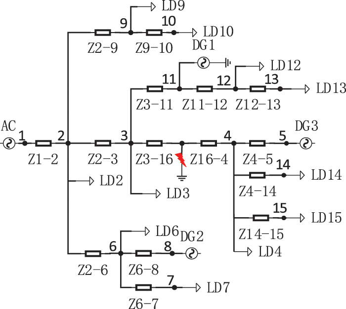
Figure 1: IEEE15 node network model

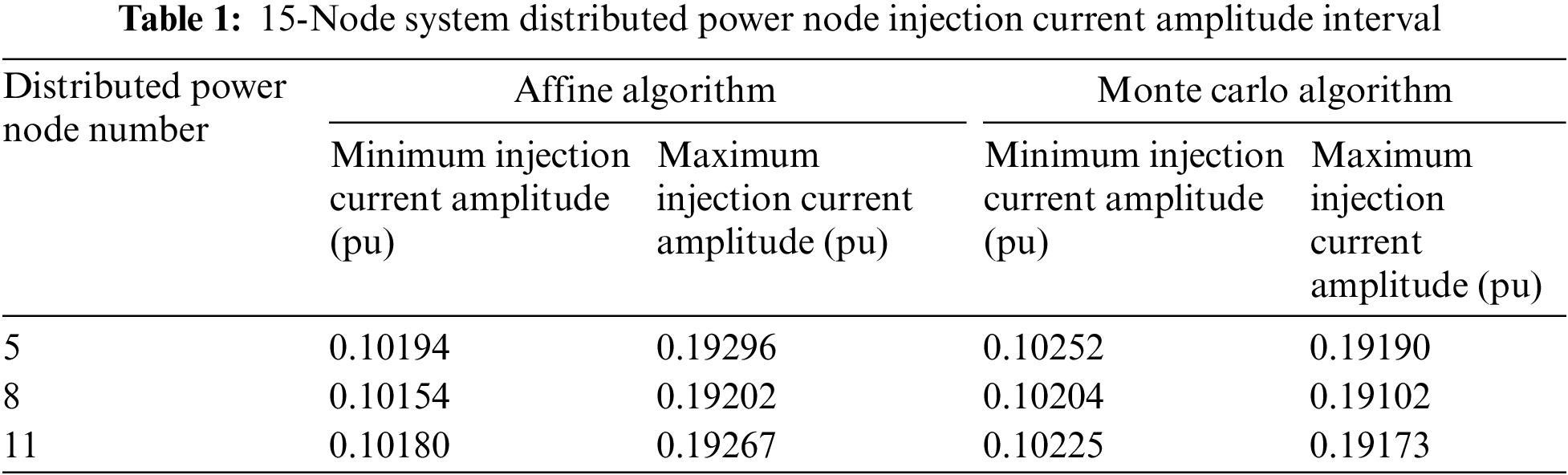
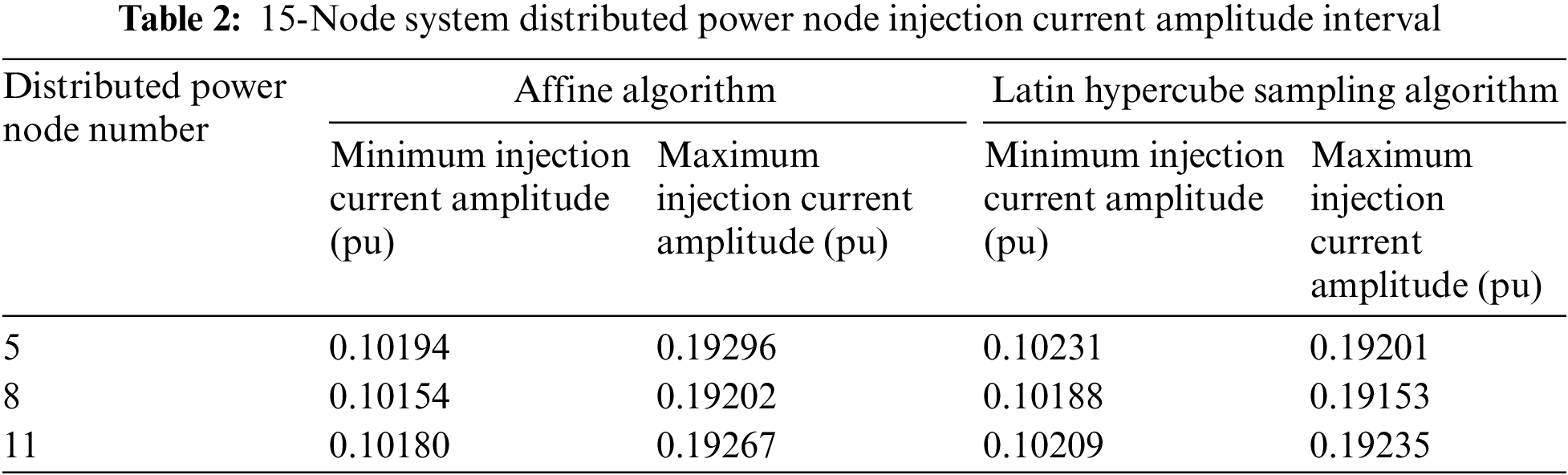
Tables 1 and 2 show the injection currents of the DG nodes. Among them are the maximum and minimum injection current amplitude calculated using the algorithm proposed in this article, Monte Carlo algorithm, and Latin hypercube sampling algorithm, respectively. The injection current amplitude intervals obtained by the affine algorithm for distributed power nodes are slightly larger than the intervals obtained by the Monte Carlo algorithm and Latin hypercube sampling algorithm.

6.2 Calculation of the Line Current Range during a Short Circuit Fault

The improved IEEE15 node system introduced in Section 6.1 is also used in this section. We assume that the fluctuation range of the active power export for each distributed power source is [−34%, +25%]. When a three-phase short circuit with a transition resistance of 10 Ω occurs at the midpoint of the 4–3 transmission line, the affine algorithm proposed in Section 5 and the Monte Carlo algorithm and Latin hypercube sampling algorithm are used to solve for the short-circuit current range of the distribution network with DGs. The SSC values after the fault are shown in Tables 3 and 4. Monte Carlo sampling and Latin hypercube sampling are applied to achieve a uniform distribution mode and to obtain 2000 random samples within the power fluctuation range.

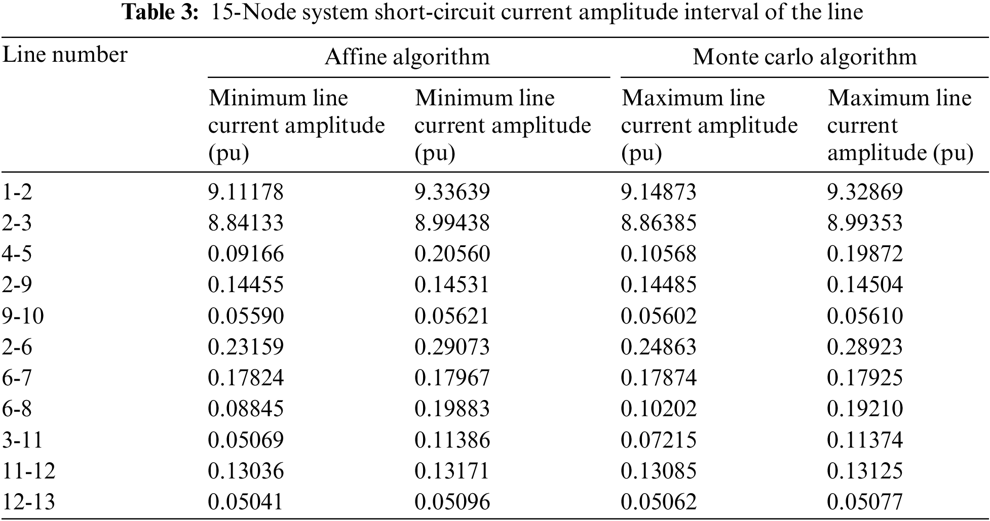
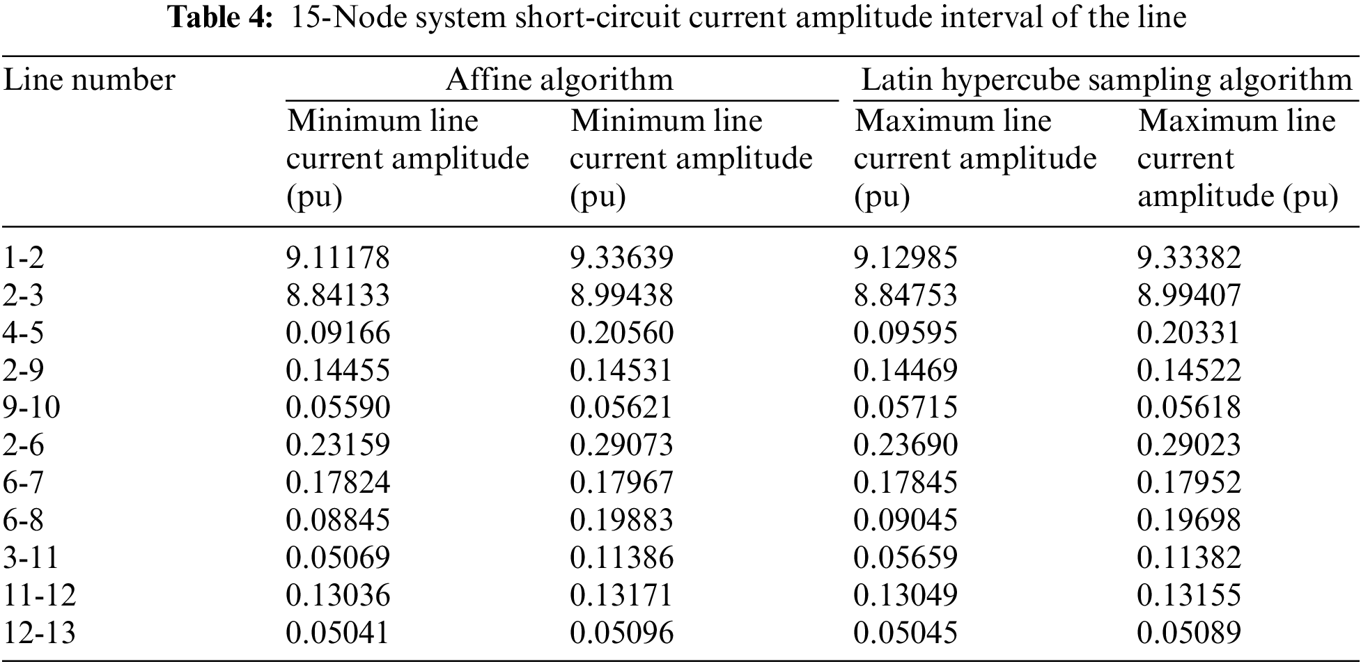
As shown in Tables 3 and 4, the short-circuit current amplitude obtained using the Latin hypercube sampling algorithm has a larger range than that obtained using the Monte Carlo algorithm. Using the affine algorithm proposed in this article, the minimum amplitude of the line current after a system short circuit is calculated to be lower than that of the Latin hypercube sampling algorithm, and the maximum amplitude of the line current is higher than that of the Latin hypercube sampling algorithm. Therefore, the affine algorithm proposed in this article calculates a larger range of short-circuit current amplitudes in the transmission line. Since the interval results obtained by the Monte Carlo algorithm are actual values, the average calculation error is defined as follows to characterize the error value of the interval results obtained by the proposed algorithm:

μx=12N∑i=1N(|x_i−x_i∗x_i∗|+|x¯i−x¯i∗x¯i∗|)(31)

where μx is the error value of the affine algorithm for the interval variable x~i; N is the number of lines; x_i and x¯i are the upper and lower bounds of the interval variables obtained by the affine algorithm; and x_i∗ and x¯i∗ are the interval variables’ upper and lower bounds obtained by the Monte Carlo algorithm.

Based on Eq. (31), the average calculation error of the affine algorithm line current interval is calculated to be 2.85%. Most errors originate from the inevitable interval expansion effect of affine interval algorithms. Additionally, some errors are caused by the linearization of trigonometric and quadratic functions using the Chebyshev approximation.

To test the performance of the proposed algorithm under different distribution node fluctuation ranges, the distributed power node’s power fluctuation range can be set to [−18%, +15%], [−34%, +25%], and [−58%, +35%]. The affine algorithm proposed in Section 5 and the Monte Carlo algorithm are used to solve the SSC range of the distribution network with DGs.

Fig. 2 shows the average error results of the upper and lower bounds for the SSC of the 15-Node system branch under different power fluctuation ranges. As the range of power fluctuations in distributed power supplies increases, the calculation error of the proposed algorithm increases.

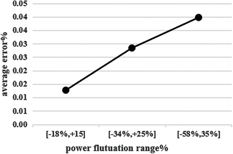
Figure 2: Average error of the short-circuit current in different fluctuation ranges

The proposed affine arithmetic algorithm is noniterative. After calculating the short-circuit current at the midpoint of the output power, the short-circuit current interval under power fluctuations can be calculated according to the affine optimization model proposed in this article. To verify the computational speed of the proposed noniterative method, calculations were performed using the proposed algorithm and the Monte Carlo algorithm and Latin hypercube sampling algorithm for the improved IEEE15 node, IEEE69 node, and IEEE118 node systems. The calculation times are shown in Table 5.

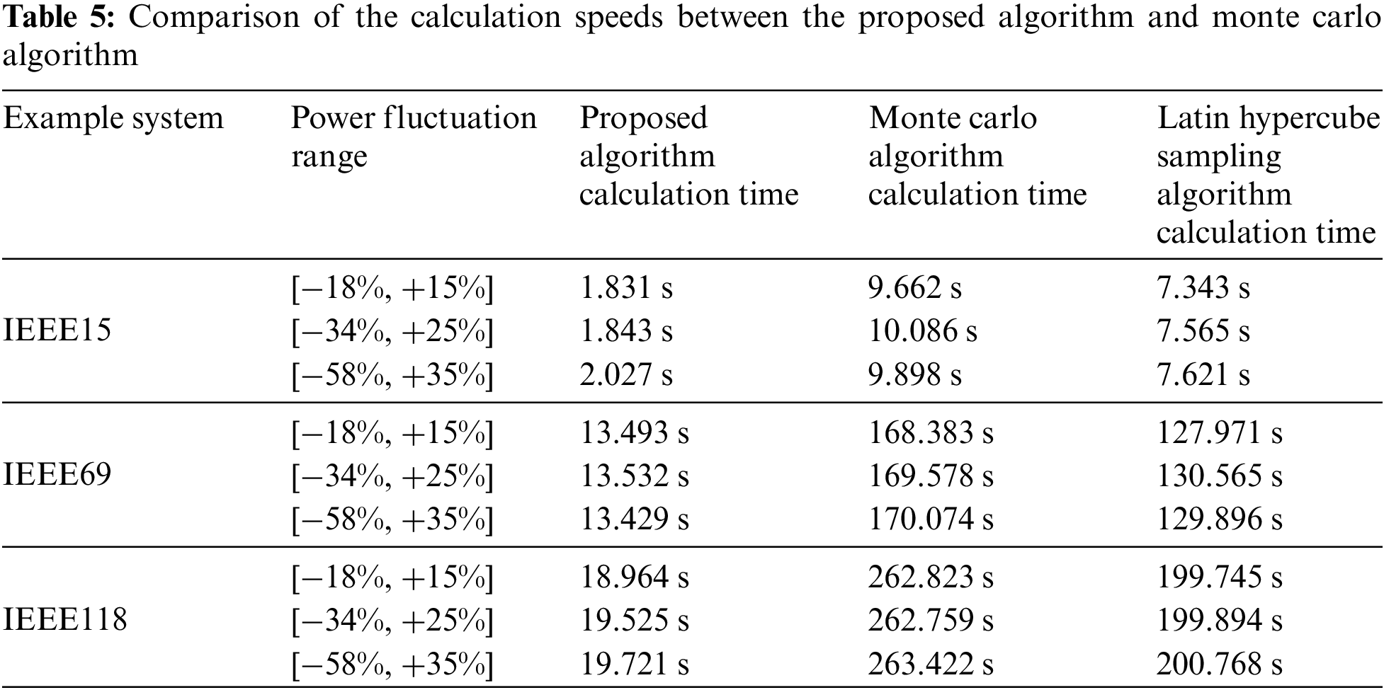
As shown in Table 5, under different fluctuation ranges in the same calculation example, the calculation times of the proposed algorithm, the Monte Carlo algorithm and the Latin hypercube sampling algorithm are not significantly different, indicating that the calculation speed is not directly related to the fluctuation range. In different examples, as the network size increases, the calculation times of the proposed algorithm, the Monte Carlo algorithm and the Latin hypercube sampling algorithm increase. However, the calculation time of the proposed algorithm is much shorter than that of the Monte Carlo algorithm and the Latin hypercube sampling algorithm. The larger the network size is, the clearer the speed improvement effect of the proposed algorithm. Therefore, the proposed algorithm has good calculation speed and is more suitable for systems with larger networks.

7  Conclusion

In this study, an affine arithmetic algorithm for calculating the SSC of distribution networks with DGs is presented. The conclusions of this study are as follows:

(1) The proposed algorithm is divided into two parts. The first establishes affine relationships between the power of the DG during normal operation and the injection current during normal operation. The second establishes affine relationships between the injection current of the DG during normal operation and the SCC after a fault occurs.

(2) Comparing the calculation results of the proposed algorithm with those of the Monte Carlo algorithm and the Latin hypercube sampling algorithm, the SCC range calculated by the proposed algorithm envelops the range obtained by the Monte Carlo algorithm and the Latin hypercube sampling algorithm; thus, the proposed algorithm has good conservatism. The lower bound of the SCC calculated by the proposed algorithm is considered slightly smaller than the lower bound of the actual value, which can be used as a basis for determining relay protection actions and fault diagnosis. The upper bound of the SCC of the line is slightly larger than the actual upper bound, which can be used as a basis for selecting and verifying robust power equipment. Thus, the algorithm proposed in this article has good practical significance for the design of power system equipment.

(3) As the power fluctuation range increases, the average calculation error of the proposed algorithm increases. However, all errors are within an acceptable range. Most errors are mainly attributed to the use of a trigonometric function and a quadratic function Chebyshev linear approximation. Compared with the Monte Carlo algorithm and the Latin hypercube sampling algorithm, the proposed algorithm significantly reduces the computational time and resource consumption.

Acknowledgement: None.

Funding Statement: This article was supported by the general project “Research on Wind and Photovoltaic Fault Characteristics and Practical Short Circuit Calculation Model” (521820200097) of Jiangxi Electric Power Company.

Author Contributions: The authors confirm the following contributions to this paper: study conception and design: Yan Zhang; data collection and methodology: Bowen Du; analysis and interpretation of results: Benren Pan and Guannan Wang; draft manuscript preparation: Guoqiang Xie and Tong Jiang. All authors reviewed the results and approved the final version of the manuscript.

Availability of Data and Materials: Data supporting this study are included within the article.

Conflicts of Interest: The authors declare that they have no conflicts of interest to report regarding the present study.

References

1. Peng, K., Zhang, C., Xu, B. Y. (2017). Key issues of fault analysis on distribution system with high-density distributed generations. Automation of Electric Power Systems, 41(24), 184–192. [Google Scholar]

2. Jia, K., Hou, L. Y., Liu, Q. (2022). Analytical calculation of transient current from an inverter-interfaced renewable energy. IEEE Transactions on Power Systems, 37(2), 1554–1563. https://doi.org/10.1109/TPWRS.2021.3107580 [Google Scholar] [CrossRef]

3. Zhang, H. Z., Li, Y. L. (2015). Short-circuit current analysis and current protection setting scheme in distribution network with photovoltaic power. Power System Technology, 39(8), 2327–2332. [Google Scholar]

4. Arani, Mohammadreza, Fakhari (2016). Assessment and enhancement of a full-scale PMSG-based wind power generator performance under faults. IEEE Transactions on Energy Conversion, 31(2), 1–12. [Google Scholar]

5. Mirhosseini, M., Pou, J., Karanayil, B. (2016). Resonant versus conventional controllers in grid-connected photovoltaic power plants under unbalanced grid voltages. IEEE Transactions on Sustainable Energy, 7(3), 1–9. [Google Scholar]

6. Yang, S., Tong, X. Q. (2016). Short-circuit current calculation of distribution network containing distributed generators with capability of low voltage ride through. Automation of Electric Power Systems, 40(11), 93–99. [Google Scholar]

7. Bi, T. S., Liu, S. M., Xue, A. C. (2016). Fault characteristics of inverter-interfaced renewable energy sources. IEEE Transactions on Sustainable Energy, 7(3), 1–9. [Google Scholar]

8. Nzimako, O., Wierckx, R. (2015). Modeling and simulation of a grid-integrated photovoltaic system using a real-time digital simulator. Clemson University Power Systems Conference (PSC), vol. 56, no. 10, pp. 89–95. IEEE. [Google Scholar]

9. Shi, T. (2018). Detailed modelling and simulations of an all-DC PMSG-based offshore wind farm. The Journal of Engineering, 8(16), 109–117. [Google Scholar]

10. Wang, L., Li, M., Deng, X. (2019). Research on modelling and simulation of converters for electromagnetic transient simulation in photovoltaic power generation system. Generation, Transmission & Distribution, IET, 13(20), 4558–4565. https://doi.org/10.1049/gtd2.v13.20 [Google Scholar] [CrossRef]

11. Wu, G. F. (2016). Three-phase short-circuit current calculation and probability assessment of power systems with photovoltaic power generations (Master Thesis). Chongqing University, China (In Chinese). [Google Scholar]

12. Li, Z. Y., Zhou, N. C., Hou, J. S. (2020). Probabilistic evaluation of short-circuit currents in active distribution grids considering low voltage ride-through uncertainty of photovoltaic. Electrical Engineering Magazine, 35(3), 564–576. [Google Scholar]

13. Qian, W. Y. (2021). Probability analysis of short-circuit current and research on critical proportion of inverter-interfaced generators connected to power system (Master Thesis). Chongqing University, China (In Chinese). [Google Scholar]

14. Pereira, L. E. S., da Costa, V. M., Rosa, A. L. S. (2012). Interval arithmetic in current injection power flow analysis. Electrical Power and Energy Systems, 43, 1106–1113. https://doi.org/10.1016/j.ijepes.2012.05.034 [Google Scholar] [CrossRef]

15. Wang, S. X., Xu, Q., Zhang, G. L. (2009). Modeling of wind speed uncertainty and interval power flow analysis for wind farms. Automation of Electric Power Systems, 33(21), 82–86. [Google Scholar]

16. Ding, T., Cui, H. T., Gu, W. (2012). An uncertainty power flow algorithm based on interval and affine arithmetic. Automation of Electric Power Systems, 36(13), 51–55+115 (In Chinese). [Google Scholar]

17. Wang, S., Wang, C., Zhang, G. (2009). Fast decoupled power flow using interval arithmetic considering uncertainty in power systems. Advances in Neural Networks-ISNN 2009, pp. 1171–1178. Wuhan, China. [Google Scholar]

18. Hu, J., Fu, L. J., Ma, F. (2016). Fast decomposition method for interval power flow in uncertain systems based on affine arithmetic optimization. Transaction of China Electrotechnical Society, 31(23), 125–131 (In Chinese). [Google Scholar]

19. Pereira L.E., S., da Costa, V. M., Rosa A.L., S. (2012). Interval arithmetic in current injection power flow analysis. International Journal of Electrical Power & Energy Systems, 43(1), 1106–1113. https://doi.org/10.1016/j.ijepes.2012.05.034 [Google Scholar] [CrossRef]

20. Pereira L.E., S., da Costa, V. M. (2014). Interval analysis applied to the maximum loading point of electric power systems considering load data uncertainties. International Journal of Electrical Power & Energy Systems, 54, 334–340. https://doi.org/10.1016/j.ijepes.2013.07.026 [Google Scholar] [CrossRef]

21. Pereira L.E., S., da Costa V, M., (2016). An efficient starting process for calculating interval power flow solutions at maximum loading point under load and line data uncertainties. International Journal of Electrical Power & Energy Systems, 80, 91–95. https://doi.org/10.1016/j.ijepes.2016.01.040 [Google Scholar] [CrossRef]

22. Liu, T. J., Jiao, W. L., Tian, X. H., Zhang, X. (2022). Dispatching optimization of city gas station district energy systems with multiple uncertainties based on an improved affine arithmetic method. Energy Reports, 9, 37–47. [Google Scholar]

23. Kim, I. (2019). Short-circuit analysis models for unbalanced inverter-based distributed generation sources and loads. IEEE Transactions on Power Systems, 34(5), 3515–3526. https://doi.org/10.1109/TPWRS.59 [Google Scholar] [CrossRef]

24. Cheng, S., Zuo, X. W., Yang, K., Wei, Z. B., Wang, R. (2022). Improved affine arithmetic-based power flow computation for distribution systems considering uncertainties. IEEE Systems Journal, 17(2), 1918–1927. [Google Scholar]

25. Zheng, W. D., Wang, X. J., Shao, Z. G., Zhang, M., Li, Y. X. (2022). A modified affine arithmetic-based interval optimization for integrated energy system with multiple uncertainties. Journal of Renewable and Sustainable Energy, 1(14), 125–136. [Google Scholar]

26. Liao, X. B. (2020). Extended affine model and its application in power system interval power flow analysis (Ph.D. Thesis). Wuhan University, China (In Chinese). [Google Scholar]

27. Gan, Y., Huang, J. W., Wu, J., Lu, H. L., Chen, J. et al. (2023). Research on probabilistic power flow calculation improvement method of power system including wind and photovoltaic power generation. Journal of Electric Power Science and Technology, 38(5), 34–43. [Google Scholar]

28. Shields, M. D., Zhang, J. (2016). The generalization of latin hypercube sampling. Reliability Engineering & System Safety, 148, 96–108. https://doi.org/10.1016/j.ress.2015.12.002 [Google Scholar] [CrossRef]