Carbon Emission Factors Prediction of Power Grid by Using Graph Attention Network

Nomenclature

1  Introduction

The continuous development of global climate change and the greenhouse effect have been acknowledged worldwide [1]. There is an international consensus to implement effective measures to reduce carbon dioxide emissions, so governments around the world have been proposing the peak of carbon emissions and the deadline for carbon neutralization [2]. In the process of reducing carbon emissions, it is crucial to reduce the carbon emitted by fossil energy combustion [3]. In the power industry, fossil energy is still dominant, which results in significant carbon emissions. The statistics of carbon emissions are typically based on macro data, several studies have identified the generational factors related to carbon emissions and have proposed carbon reduction methods based on the generational side [4–6]. Reference [6] considers the influence of environmental operating characteristics on carbon emissions of gas turbine power plants, which will help to reduce carbon dioxide emissions. However, these carbon emissions are counted on the production side, all carbon costs are eventually distributed equally to all users, which cannot encourage users to reduce carbon emissions. According to the carbon flow model [7], several demand-side-based carbon reduction methods have been proposed [8–10]. The carbon cost is distributed to each node of power grids based on certain principles, which clarify the actual carbon responsibility between power plants, power grids, and users.

The carbon flow model attaches the virtual carbon flow to the actual power flow to realize the traceability of carbon responsibility, the model defines carbon emission factors of nodes in a power grid through the weighted sum of all branch power carbon flow densities flowing into the node. However, it requires real-time parameters of power generation, loads, and power flows of the power grid. But these data cannot do real-time updates. Therefore, the existing method relies on past grid data to assess the past carbon emission factors of nodes, which makes it unable to provide users with carbon emission factors in the future.

Currently, there are few studies on predicting demand-side carbon emission factors. Load is the initial factor that affects the carbon emission factors of each node in power grids, and load prediction methods for power grids are relatively well-established and developed [11], including a statistical method based on historical data [12], artificial intelligence algorithm based on machine learning and deep learning [13–15], a combination of long-term and short-term memory [16–18] and other methods. So, a neural network model with load as input can predict the corresponding carbon emission factors in the future. Considering the spatial characteristics of carbon emission factors distribution of power grid nodes, this paper proposes a prediction model based on a graph attention network (GAT) [19], compared with a Convolutional Neural Network (CNN) [20] and Recurrent Neural Network (RNN) [21] which can deal with irregular graph structure data by adopting the same topology as the power grid. Our model designs a supervised network by training the node’s loads and its corresponding carbon emission factors data.

2  Calculation of Carbon Emission Factors Based on Tidal Flow Results and Carbon Flow Theory

2.1 Principle of Power Grid Carbon Flow Calculation

Existing carbon flow analysis methods include the proportional sharing model [22], complex power tracking method, power grid distribution method, and others. Among them, the carbon flow analysis method based on the proportional sharing method is easy and widely used to calculate. Based on the power flow calculation results, the carbon emission factors of a node in power grids can be defined. Energy consumption and carbon emissions in power grids are mainly related to the active power output of generators and are slightly affected by the reactive power output of generators. Therefore, the carbon emissions flow can be considered only affected by the system’s calculation results [23]. Based on carbon flow analysis, the carbon emission factors can be defined as the weighted sum of the active power of each branch flowing into the node. According to the principle of proportional sharing [24], the carbon emission factors of the node are calculated as Eq. (1) [24]:

δpi=Pgi⋅δgi+∑j∈Ω1Pij⋅δpjDi+∑k∈Ω2Pki(1)

where δpi and δpj(kgCO2/kWh) are carbon emission factors of nodes i and j, respectively; δgi(kgCO2/kWh) is the carbon emission factors of generators connected to node i; Pgi(kW) represents active power of generators connected to node i;Pij(kW) and Pki(kW) are active power flows of node j to node i and node i to node k, respectively, meanwhile, Ω1 is the collection of branch nodes that flow into node i, and Ω2 is the collection of branch nodes of the outflow node i; Di(kW) is the load of node i.

2.2 Solution of Carbon Emission Factors for Nodes

The following equation can be obtained by processing the Eq. (1):

(Di+∑k∈Ω2Pki)⋅δpi−∑j∈Ω1Pij⋅δpj=Pgi⋅δgi(2)

The overall expression can be written based on the calculation principle by Eq. (2):

Aδ=Eg(3)

Aij={Di+∑k∈Ω2Pki(j=i)−Pij(j∈Ω1)0(otherwise)(4)

Eg=[Eg1,⋯,Egi,⋯,Egn]T(5)

Egi=Pgi×δgi,i=1,2,⋯,n(6)

where δ(kgCO2/kWh) is the carbon emission factors vector of all nodes in a power grid; A(kW) is the solution coefficient matrix, A=[Aij]∈Rn×n; Eg(kgCO2/h) is the injected power vector of all generators; n is the number of nodes in the grid. Since Eq. (2) is a nodal energy conservation equation, Eq. (3) is the collection of n independent formulas. Eq. (3) can be changed as follows:

δ=A−1Eg(7)

From the above equations, it can be seen that the carbon emission factors of a node are only related to the load and active power flow when generators power and their carbon emission factors are known. Considering that the power flow calculation is highly dependent on the operation parameters of power grids and has problems of high complexity and long time consumption, this paper takes node loads D=(D1,D2,D3,⋯,Dd) as the input characteristics of the network model.

3  Carbon Emission Factors Prediction Based on The GAT

3.1 The GAT Principle and Its Network Design

3.1.1 Principle of GAT

The Graph Neural Network (GNN) [25] is a deep neural network model that processes structured data. Unlike traditional neural networks, GNN considers the relationships between nodes, where the core is the mutual aggregation of features between each node, then its surrounding nodes can form new node features to complete information transmission. After iteration, the GNN can obtain all the structural information of the graph. Graph Attention Network (GAT) is an important branch of GNN that considers the topological relationships between nodes in the graph and applies attention to updating feature vectors.

3.1.2 Design for GAT

1)   Topological structure of a power grid

Our model adapts topological structure same as a power grid, A graph is a representation of entities through nodes, edges, and their connections. It is comprised of three elements, namely, nodes, edges, and global information. The global information is based on nodes and edges according to a certain topological structure. Power grids are an entity consisting of transmission lines between user nodes, so their composition may correspond entirely to the graph structure. Therefore, we set the same number of nodes in the model as the power grid, then set the edges between nodes according to the distribution of power lines in the power grid. In this way, nodes can aggregate the information of neighboring nodes to fit power flows in the power grid. The carbon emission factors of the power grid are essentially the power flow of nodes, which represents the information transmission between nodes. This makes GAT suitable for structures of power grids and enables it to properly reflect the transmission characteristics of power grids.

2)   Method of updating parameters

We use multilayer GAT to build the model, which can increase the receptive area of the network [26] so that the information of the marginal nodes can be aggregated to the central node. The attention mechanism specifically integrates the information of the neighboring nodes through the attention correlation coefficient between the feature vectors. The structure of the model is shown in Fig. 1 and the specific propagation mode between the layers is as Eqs. (8)–(12) [19].

Figure 1: Structure of model

H(l+1)=(h1(l+1),h2(l+1),h3(l+1)⋯hn(l+1))(8)

hi(l+1)=σ(∑j∈NiαijW(l)hj(l))(9)

αij=exp⁡(LeakyReLu(aT[Whi||Whj])∑c∈Niexp⁡(LeakyReLu(aT[Whi||Whc])(10)

hi(l+1)=σ(1E∑e=1E∑j∈NiαijWe(l)hj(l))(11)

H(m+1)=σ(W(m)H(m)+B(m))(12)

where H(l+1) is the output feature matrix of layer l and H(l) is the input feature matrix of layer l, n is the total number of nodes in the power grid; GAT update parameters are calculated point-by-point, and Eq. (9) shows the process of this calculation, σ is the non-linear activation function with optional ReLU, softmax, etc. Ni is the set of nodes connected to the node i, αij is the attention correlation coefficient, which reflects the importance of each other by measuring the correlation of the feature vectors of two nodes, that will determine the weighted value of different connections when the node features are aggregated. W is a learnable weight matrix whose function is to convert the dimension of the input feature vector into the output dimension; αij can be calculated by Eq. (10), aT is a weight vector and it can transform the two feature vectors into a one-dimensional correlation coefficient by multiplying with the splice vector Whi||Whj, then we can introduce LeakyReLu for nonlinear activation. To compare the correlation coefficients, different correlation coefficients connected to node i are regularized by the softmax; Eq. (11) introduces a multi-head mechanism, which adds E-1 channel relative to Eq. (9), and the average value of all channels is taken as the final output result.

After the last graph attention layer, the full connection layer is connected to organize the output characteristics and adjust the output dimensions for the prediction task. Eq. (12) is the mode of propagation between the fully connected layers, H1 is the output of the input layer of the fully connected layer and the last layer of GAT. W(m) is the weight vector of layer m, B(m) is the bias vector of layer m, the former is a non-shared parameter while the latter is a shared parameter.

3)   Evaluating indicator

The backpropagation algorithm is a common and effective parameter updating method based on supervised loss. Because the predicted carbon emission factors of the power grid are small, the error value is generally less than 1, which makes the mean square error function (MSE) slow in this range. Therefore, the mean absolute error (MAE) can be trained as a loss function, and MAPE is an indicator to evaluate the effect of the model as follows:

MAE=1n∑i=1n|y~i−yi|(13)

MAPE=100%n∑i=1n|y^i−yiyi|(14)

where y~i and yi indicate the predicted and true values of the carbon factors at node i, respectively, n is the number of samples of the data set.

3.1.3 Training Method

In this paper, the gradient descent method of the small batch is used to train the prediction model. For the convenience of training, setting the batch size of samples, and then the corresponding network parameters updated according to the gradient descent direction of a batch can avoid the fluctuation of the descent direction.

3.2 Procedure of Carbon Emission Factors Prediction

The prediction process can be divided into four steps which are shown in Fig. 2.

Figure 2: Procedure of carbon emission factors prediction

•   Fixed loads from the standard test system are used as means, and 30% of means as the variance generate a random load sequence to provide the load data for power flow calculation;

•   Based on the random load sequence and power generation data, power flow is analyzed, then the theoretical carbon emission factors of each node are calculated according to the carbon emissions flow data (regarded as the theoretical value);

•   The GAN model is trained offline using the load data (input) generated in Step 1 and the carbon emission factors data (output) calculated in Step 3. The best epoch is generated according to the results of the test set, and then the model of the best epoch is used as the best model.

•   The load to be predicted is input into the prediction model trained offline in Step 3 to realize the online prediction of carbon emission factors in the power grid.

4  Test Analyse

4.1 Data Specification

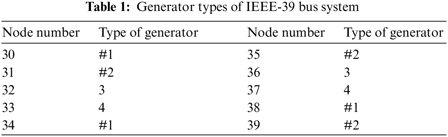
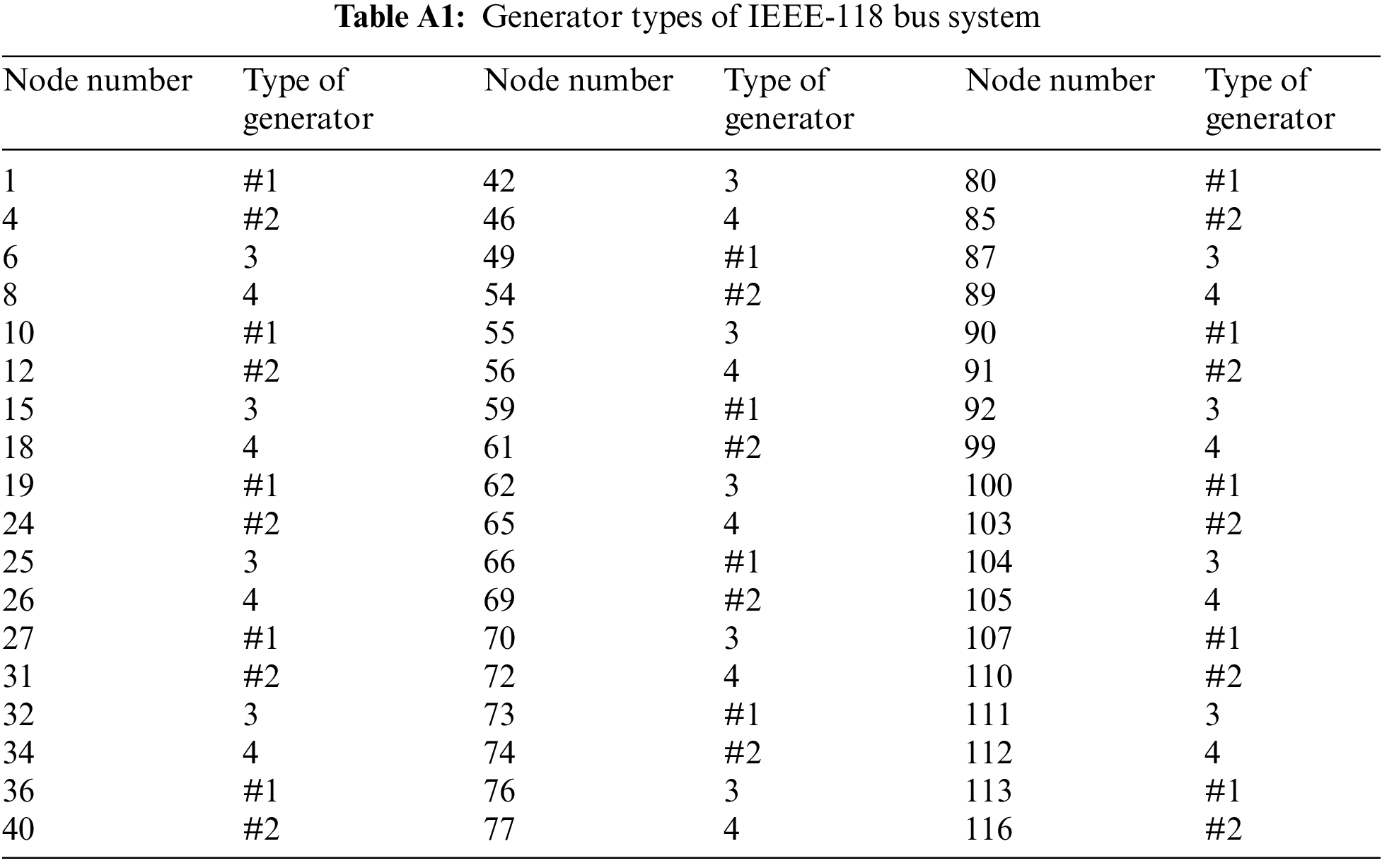
Generator set: In this paper, four types of generator sets are used in the IEEE-39 bus and IEEE-118 bus systems to verify the effectiveness of the proposed method. The four types of generating units include coal-fired unit #1, coal-fired unit #2, gas unit, and hydropower unit, with carbon emissions intensity of 1.5, 0.95, 0.5, and 0 (kg/kWh) [27], respectively.

Input data: Due to a lack of actual load data, we generated an input data set with a dimension of 10000 × n, where 10000 is the number of samples and n is the number of nodes in the test grid. The specific process is as follows: Taking the default load values of each node given by “case39” and “case118” [28,29] in MATPOWER as the mean values, then generate 10000 groups of random normal distribution sequences with 30% of the mean values as the variance. Considering that some nodes in the power grid have no load, the columns corresponding to these nodes are supplemented with 0, so the dimension of the load data set reaches 10000 × n. The 10000 sets of training data are randomly divided into a training set, a validation set, and a test set according to 7:2:1.

4.2 Test for IEEE-39 Bus System

4.2.1 Parameter Settings for IEEE-39 Bus System

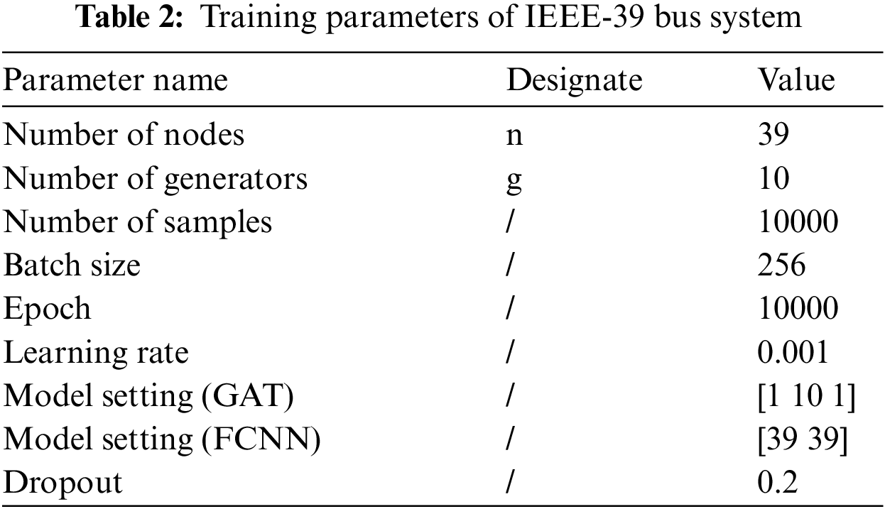
The generator typesetting of the IEEE-39 bus system is shown in Table 1 and the network training parameters are shown in Table 2.

4.2.2 Test Results of IEEE-39 Bus System

The effectiveness of GAT in predicting the node carbon emission factors is tested using the IEEE-39 bus system. Due to the excessive number of nodes in the system, typical nodes are selected based on their representativeness. The degree (degree represents the number of neighboring nodes) of each node in the IEEE-39 bus system is shown in Fig. A1 of Appendix A. Node 16 has the highest degree, indicating that it is the central node, this kind of node is a hub node in the actual power grid, and its power flow is easily influenced by the surrounding nodes, so its carbon emission factors fluctuate greatly. The node 39 is connected to the generator and has a large load, which makes it a complex node. This kind of node is close to the generator in the actual power grid, when its load is greater than the input power of the connected generator, the carbon emission factors will also be affected by the carbon emission factors of other nodes, otherwise, the carbon emission factors of this node will be consistent with the power generation carbon emissions intensity of the generator. Additionally, there is a typical class of nodes (such as node 10), whose carbon emission factors do not change with the load. Therefore, they are selected as typical nodes for analysis.

Fig. 3 presents a comparison between the predicted values and the true values (the top 50 samples of the test set) in the dataset. The prediction error rates of nodes 39 and 10 are overall at a low level, but that of node 16 is slightly larger. Specifically, the MAPE of the three typical nodes is 4.63%, 1.20%, and 0.06%, respectively.

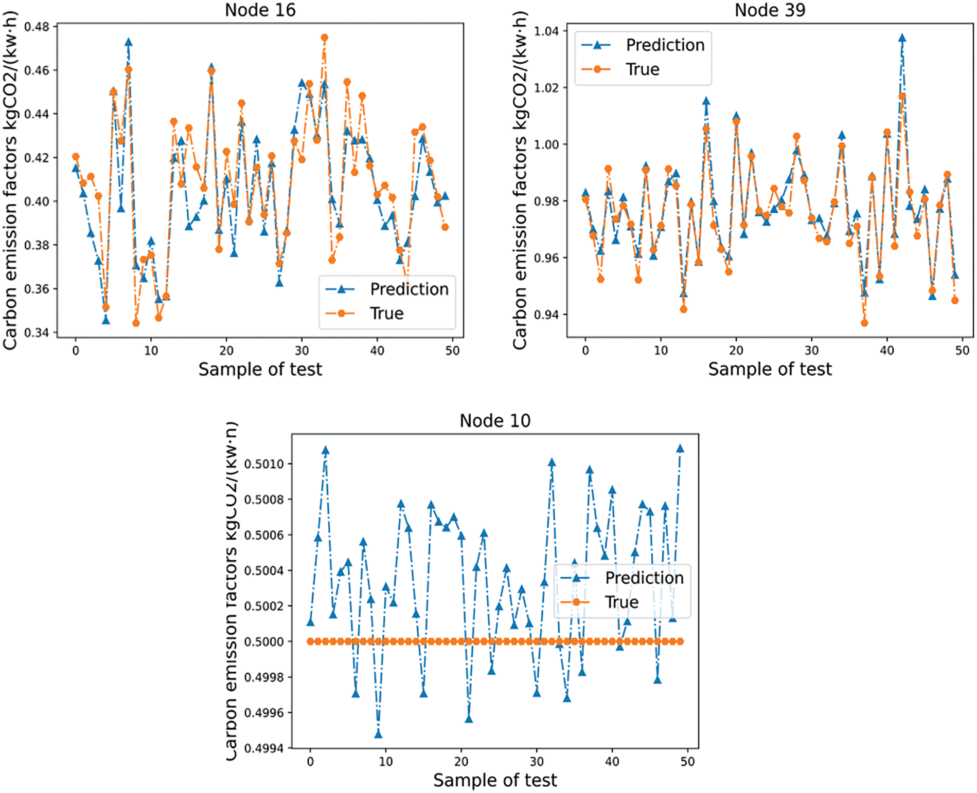
Figure 3: Prediction of carbon emission factors of some nodes in IEEE-39 bus system

To illustrate the prediction results more intuitively, a 3D scatter plot is drawn in Fig. 4, where blue and red scatter points are test samples and predicted carbon emission factors values, respectively. Due to a large number of nodes, only some nodes are displayed. Fig. 5 is a violin figure that presents the distribution of the prediction error rates for all the nodes, The wider width of the x-axis direction represents the greater corresponding error rate, and four lines in the graph represent the maximum, mean, median, and minimum. It shows that most node’s prediction error values are below 10%, the maximum error rate is 17.5% and the relative average error between them is only 2.46%. In conclusion, This model achieves an average node prediction error rate of less than 5% and a maximum node prediction error rate of less than 20% under the dataset of this paper.

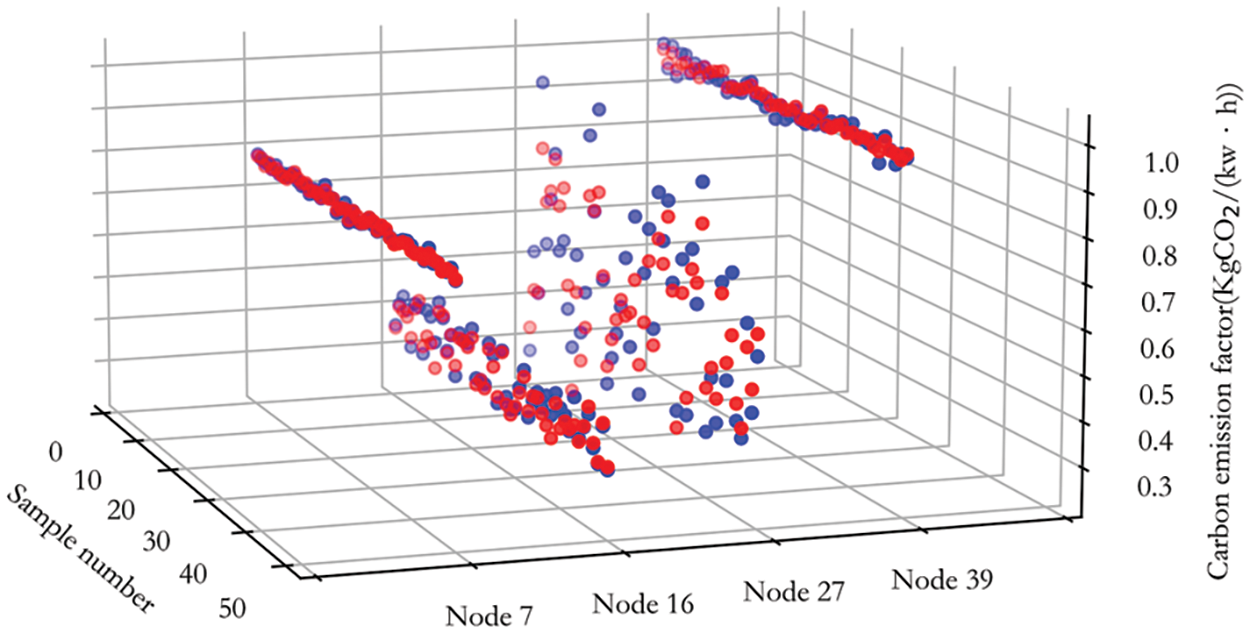
Figure 4: 3D scatter plot of partial nodes in IEEE-39 bus system

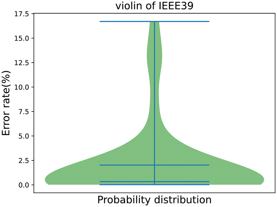
Figure 5: Forecast radar chart of IEEE-39 bus system

4.3 Test for IEEE-118 Bus System

4.3.1 Parameter Settings for IEEE-118 Bus System

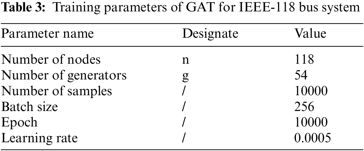
The number of generator nodes and complexity of nodes in the IEEE-118 bus system have been greatly improved compared with the 39 system. Types and settings of generators in the system are given in Table A1 of Appendix A. The network training parameters are shown in Table 3, and the training parameters of the contrast algorithm are shown in parentheses.

4.3.2 Test Results of IEEE-118 Bus System

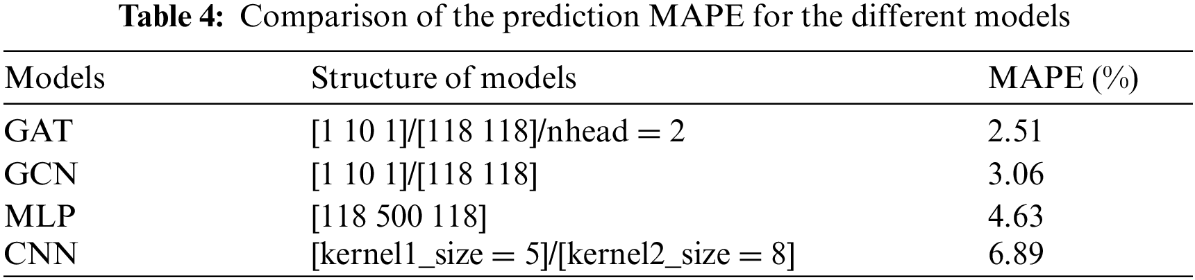
To objectively evaluate the effectiveness of the proposed method, Table 4 statistics the MAPE of MLP, GCN [30,31], and GAT with the same dataset. We can see that using the GAT model yielded a minimum MAPE of 2%, The largest is the MLP model whose value reaches 4.63%.

Similar to the IEEE-39 bus system, the degrees of each node in the IEEE-118 bus system are shown in Fig. A2 of Appendix A. The selected typical nodes are 59 (complex node), 49 (central node), and 62 (carbon emission factors constant node). MAPE of the three typical nodes is 0.55%, 0.20%, and 1.82%, respectively, The prediction results of each typical node are similar to those in the IEEE-39 bus system, as shown in Fig. 6, the scatter plots of some nodes are shown in Fig. 7.

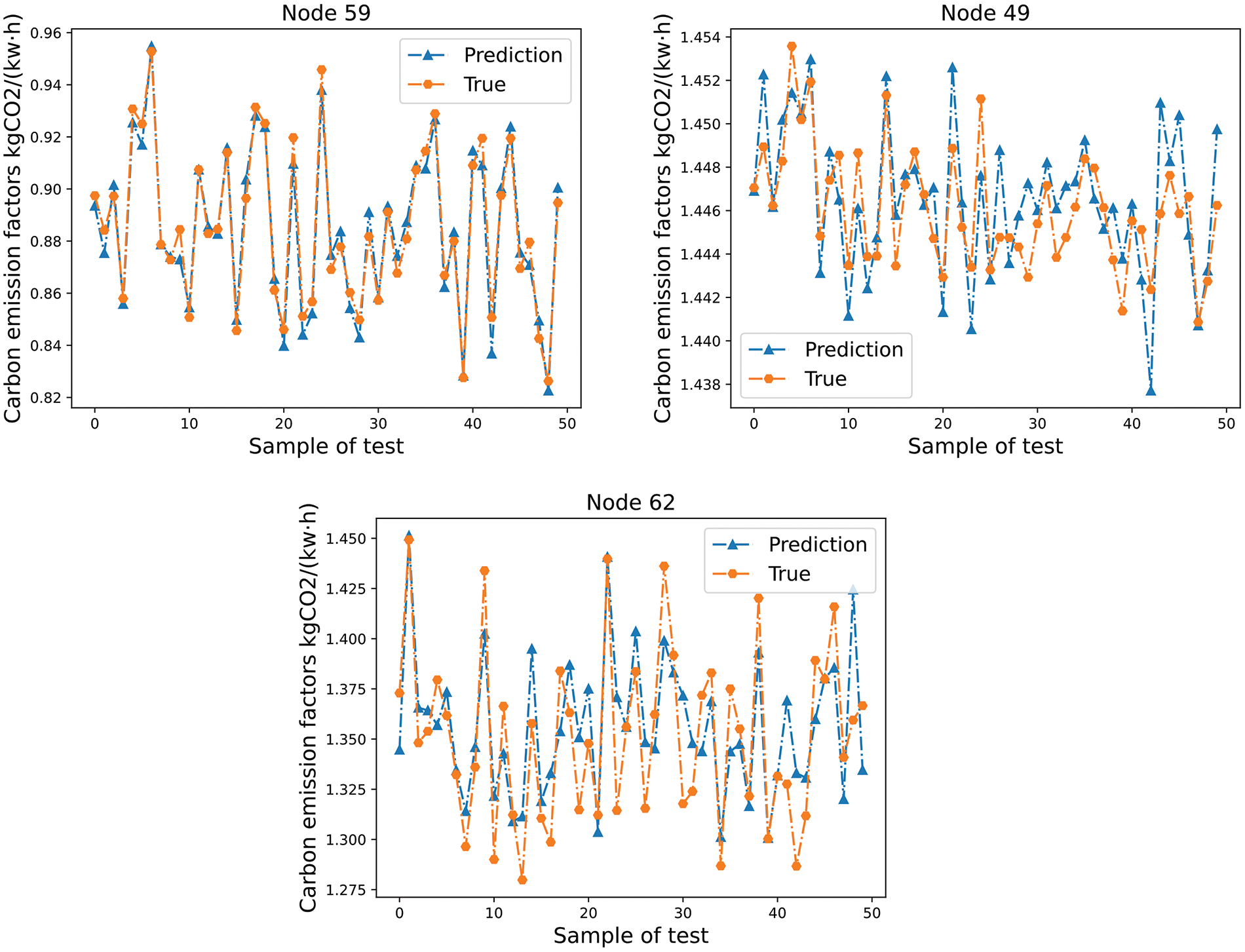
Figure 6: Prediction of carbon emission factors of some nodes in the IEEE-118 bus system

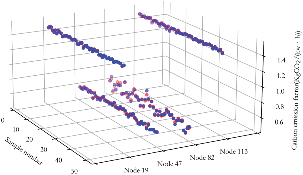
Figure 7: 3D scatter plot of partial nodes in IEEE-118 bus system

Fig. 8 shows that the prediction error values of most nodes are below 10%, the maximum error rate is 30% and the relative average error between them is only 2.51%, which indicates that the GAT is still effective in large-scale node systems.

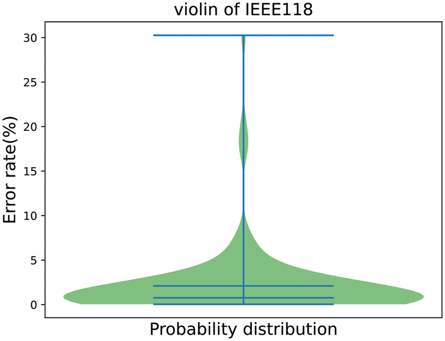
Figure 8: Forecast radar chart of IEEE-118 bus system

4.4 Practical Implications

The carbon responsibility allocation system with carbon emission factors as the core can activate the demand-side carbon reduction power. Put the future load data of each node into the forecasting model, and output the carbon emission factors data of each node in the future, which can give users a reference for carbon reduction, when the carbon emission factors are low at a certain moment, users can move the peak of electricity consumption to this period to reduce the overall carbon emissions. At present, this paper has only done preliminary work on the prediction method of load-carbon emission factors, which is still far from practical application. The possible application steps that the author thinks are as follows: First, the parameters for theoretical calculation should be accurate and complete, such as power grid operation parameters, generator power data, and load data, all the parameters needed for database processing are established to ensure the timeliness of data; Secondly, different models are trained to cope with different system topologies caused by different operating scenarios; Predicting the load data in the future is the key link in practical application; The prediction accuracy of the model should be evaluated, which gives a reference for the adjustment of model parameters.

5  Conclusion

Because of the current power carbon emission factors calculation methods have serious assessment characteristics, which make it impossible to provide power grid and users with prospective guidance. This paper proposes a node carbon emission factors prediction method based on GAT, which puts the grid topology into the neural network to build a supervised prediction model. Based on the example analysis of the IEEE-39 bus and IEEE-118 bus systems, the following conclusions can be obtained:

GAT integrated into the topology information of a power grid can effectively extract the feature information of nodes, and then learn the interrelationship between nodes. Lastly, it achieves better prediction results than MLP, GCN, and CNN.

The prediction method based on GAT achieves similar prediction results and performance in IEEE-39 bus and IEEE-118 bus systems, which shows that the model is scalable and easy to migrate.

It must be pointed out that the load data used in this model are randomly generated according to the normal distribution, and the actual load distribution law has not been taken into account. The setting of carbon emissions intensity of generators in the test system is relatively traditional. In future work, we will improve the quality of the load data set and consider introducing a high proportion of new energy generators.

Acknowledgement: We want to thank for the help of Dr. Zhang and Dr. Guo.

Funding Statement: This work is supposed by the Science and Technology Projects of China Southern Power Grid (YNKJXM20222402).

Author Contributions: The authors confirm contribution to the paper as follows: conceptualization and investigation: Xin Shen, Weibin Lin; formal analysis: Xin Shen, Yujun Yin; methodology: Mi Zhou; project administration: Jianlin Tang; resources: Jianlin Tang; software: Yujun Yin; supervision: Jiahao Li, Yujun Yin; validation: Weibin Lin, Mi Zhou; draft manuscript preparation: Xin Shen, Jiahao Li, Jianlin Tang, Mi Zhou. All authors reviewed the results and approved the final version of the manuscript.

Availability of Data and Materials: The authors confirm that the data used in this study are available on request.

Conflicts of Interest: The authors declare that they have no conflicts of interest to report regarding the present study.

References

1. Mateos, R. M., Sarro, R., Díez-Herrero, A., Reyes-Carmona, C., López-Vinielles, J. et al. (2023). Assessment of the socio-economic impacts of extreme weather events on the coast of Southwest Europe during the period 2009–2020. Applied Sciences, 13(4), 2640. https://doi.org/10.3390/app13042640 [Google Scholar] [CrossRef]

2. Yao, J., Han, H., Yang, Y., Song, Y., Li, G. (2023). A review of recent progress of carbon capture, utilization, and storage (CCUS) in China. Applied Sciences, 13(2), 1169. https://doi.org/10.3390/app13021169 [Google Scholar] [CrossRef]

3. Zhao, X., Luo, D. (2018). Forecasting fossil energy consumption structure toward low-carbon and sustainable economy in China: Evidence and policy responses. Energy Strategy Reviews, 22, 303–312. [Google Scholar]

4. Dehghani-Sanij, A., Kashkooli, F. M. (2023). Special issue: New developments and prospects in clean and renewable energies. Applied Sciences, 13(17), 9632. https://doi.org/10.3390/app13179632 [Google Scholar] [CrossRef]

5. Pourakbari-Kasmaei, M., Lehtonen, M., Contreras, J., Mantovani, J. R. S. (2019). Carbon footprint management: A pathway toward smart emissions abatement. IEEE Transactions on Industrial Informatics, 16(2), 935–948. [Google Scholar]

6. Egware, H. O., Kwasi-Effah, C. C. (2023). A novel empirical model for predicting the carbon dioxide emissions of a gas turbine power plant. Heliyon, 9(3), e14646. https://doi.org/10.1016/j.heliyon.2023.e14645 [Google Scholar] [PubMed] [CrossRef]

7. Kang, C., Zhou, T., Chen, Q., Xu, Q., Xia, Q. et al. (2012). Carbon emissions flow in networks. Scientific Reports, 2, 479. https://doi.org/10.1038/srep00479 [Google Scholar] [PubMed] [CrossRef]

8. Coskun, C. (2019). A time-varying carbon intensity approach for demand-side management strategies with respect to CO2 emissions reduction in the electricity grid. International Journal of Global Warming, 19(1–2), 3–23. [Google Scholar]

9. Sarker, E., Halder, P., Seyedmahmoudian, M., Jamei, E., Horan, B. et al. (2021). Progress on the demand side management in smart grid and optimization approaches. International Journal of Energy Research, 45(1), 36–64. [Google Scholar]

10. Feng, J., Nan, J., Wang, C., Sun, K., Deng, X. et al. (2022). Source-load coordinated low-carbon economic dispatch of electric-gas integrated energy system based on carbon emissions flow theory. Energies, 15(10), 3641. https://doi.org/10.3390/en15103641 [Google Scholar] [CrossRef]

11. Ghulam, H., Khurram, S., Alimgeer, I. K. (2020). Electric load forecasting based on deep learning and optimized by heuristic algorithm in smart grid. Applied Energy, 269, 114915. https://doi.org/10.1016/j.apenergy.2020.114915 [Google Scholar] [CrossRef]

12. Nti, I. K., Teimeh, M., Nyarko-Boateng, O. (2020). Electricity load forecasting: A systematic review. Journal of Electrical Systems and Information Technology, 7, 13. https://doi.org/10.1186/s43067-020-00021-8 [Google Scholar] [CrossRef]

13. Wu, W. T., Li, P., Liu, R. H., Jin, W. Z., Yao, B. Z. et al. (2020). Predicting peak load of bus routes with supply optimization and scaled Shepard interpolation: A newsvendor model. Transportation Research Part E: Logistics and Transportation Review, 142, 102041. https://doi.org/10.1016/j.tre.2020.102041 [Google Scholar] [CrossRef]

14. Wu, W. T., Lin, Y., Liu, R. H., Jin, W. Z. (2022). The multi-depot electric vehicle scheduling problem with power grid characteristics. Transportation Research Part B: Methodological, 155, 322–347. [Google Scholar]

15. Chahikoutahi, F., Khashei, M. (2017). A seasonal direct optimal hybrid model of computational intelligence and soft computing techniques for electricity load forecasting. Energy, 140, 988–1004. [Google Scholar]

16. Dietrich, B., Walthe, J., Weigold, M., Abele, E. (2020). Machine learning based very short term load forecasting of machine tools. Applied Energy, 276, 115440. https://doi.org/10.1016/j.apenergy.2020.115440 [Google Scholar] [CrossRef]

17. Yin, L. F., Xie, J. X. (2021). Multi-temporal-spatial-scale temporal convolution network for short-term load forecasting forecasting of power system. Applied Energy, 283, 116–128. [Google Scholar]

18. Wang, J. Q., Du, Y., Wang, J. (2020). LSTM based long-term energy consumption prediction with periodicity. Energy, 197, 117–197. [Google Scholar]

19. Veličković, P., Cucurull, G., Casanova, A., Romero, A., Lio, P. et al. (2017). Graph attention networks. https://arxiv.org/abs/1710.10903 (accessed on 02/01/2024). [Google Scholar]

20. Teja, K., Jens, L., Felix, S., Stefan, H. (2021). Review on convolutional neural networks (CNN) in vegetation remote sensing. ISPRS Journal of Photo Grammetry and Remote Sensing, 173, 24–49. [Google Scholar]

21. Li, S., Li, W. Q., Chris, C., Zhu, C., Gao, Y. B. (2018). Independently recurrent neural network (IndRNNBuilding a longer and deeper RNN. Proceedings of the IEEE Conference on Computer Vision and Pattern Recognition (CVPR), pp. 5457–5466. Salt Lake City, USA. [Google Scholar]

22. Liu, Y. L., Li, Y. W., Zhou, C. L. (2023). Summary of carbon emissions measurement and analysis methods in power system (In Chinese). https://doi.org/10.13334/j.0258-8013.pcsee.223452 [Google Scholar] [CrossRef]

23. Zhou, T. R., Kang, C. Q., Xu, Q. Y. (2012). Discussion on the calculation method of carbon emissions flow in power system. Power System Automation, 36(11), 44–49 (In Chinese). [Google Scholar]

24. Nyamdash, B., Denny, E. (2013). The impact of electricity storage on wholesale electricity prices. Energy Policy, 58, 6–16. [Google Scholar]

25. Scarselli, F., Gori, M., Tsoi, A. C. (2009). The graph neural network model. IEEE Transactions on Neural Networks, 20(1), 61–80 [Google Scholar] [PubMed]

26. Chen, J. F., Zhu, J., Song, L. (2018). Stochastic training of graph convolutional networks with variance reduction. Proceeding of the International Conference on Machine Learning, pp. 941–949. New York, USA. [Google Scholar]

27. Zhang, X. S., Yu, T., Yang, B., Zheng, L. M., Huang, L. N. (2015). Approximate ideal multi-objective solution Q(λ) learning for optimal carbon-energy combined-flow in multi-energy power systems. Energy Conversion and Management, 106, 543–556. [Google Scholar]

28. Zimmerman, R. D., Murillo-Sánchez, C. E., Thomas, R. J. (2011). MATPOWER: Steady-state operations, planning and analysis tools for power systems re-search and education power systems. IEEE Transactions on Power System, 26, 12–19. [Google Scholar]

29. Zimmerman, R. D., Murillo-Sánchez, C. E. (2022). MATPOWER (Version 7.0) [Software]. https://doi.org/10.5281/zenodo.32365351.1 [Google Scholar] [CrossRef]

30. Zhang, S., Tong, H., Xu, J., Maciejewski, R. (2019). Graph convolutional networks: A comprehensive review. Computational Social Networks, 6(1), 1–23. [Google Scholar]

31. Wu, F., Souza, A., Zhang, T., Yu, T., Weinberger, K. (2019). Simplifying graph convolutional networks. International Conference on Machine Learning, pp. 6861–6871. Los Angeles, USA. [Google Scholar]

Appendix A

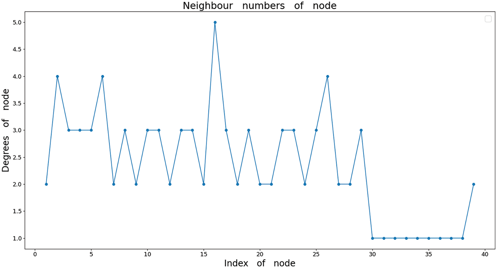
Figure A1: Degrees of nodes in IEEE-39 bus system

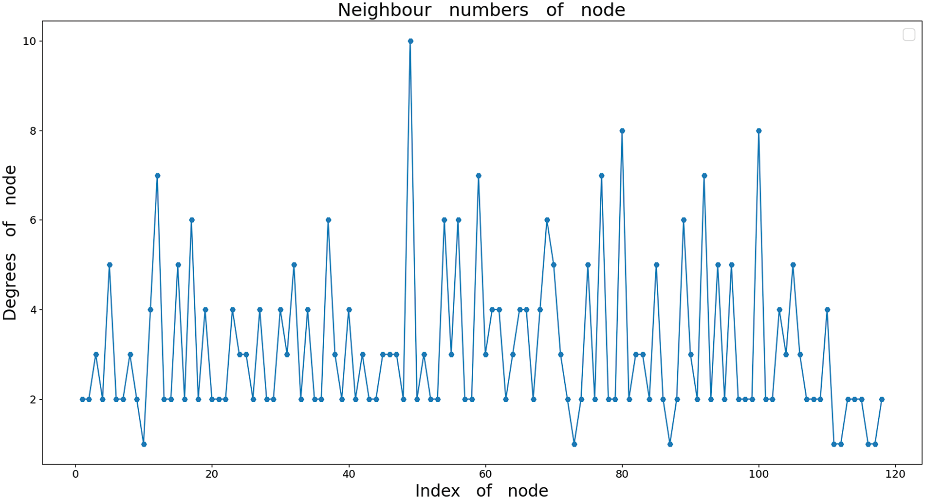
Figure A2: Degrees of nodes in IEEE-118 bus system