Migratable Power System Transient Stability Assessment Method Based on Improved XGBoost

1  Introduction

The rapid development of new energy poses a severe challenge to the stability of traditional power systems. The emerging power systems exhibit characteristics of a high proportion of new energy sources and a high proportion of power electronics [1]. The uncertainty in the grid has increased dramatically, making it crucial to identify the system operating state quickly and accurately to ensure the safety and stability of the power system. Although traditional time-domain simulation methods can accurately locate faults [2], the complexity and computation time increase exponentially with the enlargement of the power grid due to its high-dimensional nonlinear nature. Additionally, different power networks require re-modeling, further complicating the process. Therefore, there is an urgent need to introduce a transient stability assessment (TSA) method that combines speed, accuracy, and universality.

With the rapid development of artificial intelligence technology and measurement tools such as phase measurement units (PMUs), it has been support for research on data-driven TSA of power systems. Many scholars have conducted research on algorithms and data [3–5]. The data-driven TSA mainly includes offline training and online mapping. In the offline training stage, the preprocessed data is input into the machine learning model and tested for improvement to obtain the TSA model. In terms of algorithms, reference [6] employs deep random forest as a classification model. Compared to deep neural networks, it has simpler parameter settings and faster training speed. However, it also suffers from high computational complexity, sensitivity to noise, and a tendency to overfit. Reference [7] constructs a support vector machine based on a key sample set, which reduces the number of unstable samples being classified as stable. However, it has low efficiency when dealing with massive measurement data in power systems. Reference [8] builds a bidirectional long short-term memory network based on the temporal characteristics of transient process data in power systems, establishing a nonlinear mapping relationship between the underlying measurement data and the transient stability categories. However, due to the need for calculations in both forward and backward directions, the computational complexity and time required are large, making it difficult to meet the timeliness requirements of online applications. In reference [9], a real-time prediction model for power system transient stability after faults based on EOS-ELM is established by integrating OS-extreme learning machines and online boosting algorithms. What’s more, existing research generally fails to consider the increased misjudgment rate of models due to sample imbalance. Minority class samples often play a crucial role in model decision boundaries, significantly affecting the reliability of transient stability assessment results [10]. Additionally, when there are changes in the system’s topology and operating conditions, the existing research lacks adaptive generalization capabilities and fails to meet the requirements of fast online assessment.

In terms of data, the information collected in real-time by PMUs in the power grid often contains some noise, resulting in random errors between the measurement data and the true values. This increases the risk of overfitting in TSA models, making the selection of high-quality input features a prerequisite for accurate assessment [11]. Reference [12] employs an attention mechanism and utilizes a soft threshold function to automatically learn noise thresholds, reducing noise and irrelevant feature interference. However, when the data scale becomes large, the computation of attention factors becomes more complex. The reference [13] utilizes stacked sparse denoising autoencoders to reduce the interference of noise in the input data on feature extraction. However, it fails to fundamentally eliminate the noise, making it difficult to ensure the robustness of the model to noise under various operating conditions. The reference [14] addresses the issue of insufficient sample diversity by alternately training and learning the distribution characteristics of transient data, generating new samples that conform to the real distribution. But the generative-adversarial process requires a significant amount of time and is difficult to adapt to the real-time requirements of the power grid. The reference [15] introduces a histogram algorithm to discretize the original data, enhancing the model’s robustness to noise and reducing the risk of overfitting in noisy environments. However, it fails to consider the impact of sample imbalance on model evaluation. The reference [16] creates an initial dataset based on real-time dynamic information captured by PMUs, using a time set for sample labeling, and employs a least squares generative adversarial network for data augmentation, achieving effective data augmentation on a small-scale dataset. In summary, existing literature has not fundamentally addressed the detection of outliers and anomalies, and it cannot guarantee that artificially generated samples conform to the original time series distribution, which can easily interfere with the transient stability evaluation of the model.

In response to the practical problems of low quality of actual collected data, insufficient mining of minority class samples, and weak generalization ability in existing research on transient stability assessment, this paper proposes a transferable transient stability assessment method based on the XGBoost model. The main contributions of the paper are highlighted as follows:

1.    At the data level, to avoid noise interference, a data augmentation method based on the gradient detector (GD) is employed to eliminate the influence of extreme outliers on the model evaluation.

2.    At the model level, the paper proposes an improved transient stability assessment method for XGBoost. A regularization term is added to the original algorithm to prevent overfitting, and the focal loss (FL) function is introduced to guide the model training [17], thereby enhancing the mining of minority class samples.

3.    A transfer learning approach based on model parameters and sample augmentation is introduced. By fine-tuning the model parameters and augmenting the samples, the generalization ability of the model to changes in the power system’s topology and operating conditions is enhanced.

Overall, this paper presents a comprehensive approach based on the XGBoost model for transient stability assessment. It addresses the challenges of minority class sample exploration, noise interference, and generalization to different scenarios, providing an effective and accurate solution for power system stability evaluation.

This paper is organized as follows. In Section 2, a sample feature enhancement strategy is proposed for feature screening and noise interference elimination. In Section 3, The improved XGBoost model has been introduced, achieving a focus on minority class samples. In Section 4, a complete transient stability assessment process based on improved XGBoost has been introduced. Section 5 introduces the implementation of the proposed method in the IEEE 39 example. The conclusion is presented in Section 6.

2  Sample-Feature Enhancement Strategy

With the large-scale deployment of measurement components in power systems, an increasing amount of operational data can be collected and aggregated in real-time [18]. However, on the one hand, the data may be subject to noise and errors during measurement and transmission, which can affect the model’s ability to identify the power system’s operating state. On the other hand, collecting too many features can easily lead to the curse of dimensionality, reducing the efficiency of the model [19]. Therefore, the support vector machine algorithm is used to detect and correct bad data, in order to reduce the impact of bad data on situational awareness.

2.1 Sample Denoising

Taking advantage of the small magnitude of changes in the nearby region in a time series, the rolling standard deviation (RSD) approach is used. This approach involves sliding a fixed-length time window forward and, for each segment, calculating its mean and standard deviation. This process is represented by Eq. (1).

si=1t[(x1−x¯i)2+(x2−x¯i)2+…+(xt−x¯i)2](1)

In Eq. (1), i represents the window number; t represents the sliding time window length; x1…xt represents the feature value; x¯i is the average feature value of the segment, and si characterizes the degree of feature dispersion. If the data falls outside a certain multiple of the standard deviation of a sequence, the sample is likely to be an extreme outlier caused by noise interference and needs to be removed promptly to avoid affecting model evaluation. Compared with the currently used global outlier detection methods, this approach retains the trend of changes in power system time series, considers the differences in feature values caused by different states, maximizes the integrity of normal data, and the smaller the window length t, the more accurate the results.

2.2 Feature Dimension Reduction

Feature selection is crucial for evaluating the predictive accuracy of a model. However, the high-dimensional data obtained from PMU direct measurements can lead to the curse of dimensionality, increasing the time required for online evaluation and reducing the interpretability of the model. The principles of feature selection are as follows [20]: (1) The selected feature subset has a strong correlation with the target variable, meaning that the introduction of features can significantly reduce the confusion of label classification. (2) The features within the feature subset have low redundancy, so that the number of features is minimized without affecting accuracy.

Given a set of input variables X={x1,x.,…,xm} and an output variable y, the objective function for selecting the optimal feature subset using the incremental method can be expressed as:

x∗=arg⁡maxxα∈X−XSI({X,xα};y)(2)

where x∗ represents the feature to be added; xα is the set of remaining features, XS represents the target feature subset, and I(XS;y) represents the mutual information between feature subset XS and y, which represents the reduction in uncertainty of the target variable given the feature. Considering the principle of minimum redundancy and maximum relevance, the feature selection strategy can be equivalently expressed as:

x∗=arg⁡maxxα∈X−XS[I(xα;y)−∑xi∈XSI(xi;xα)](3)

Based on determining the optimal feature dimension, the selection of each feature is based on its contribution to the model evaluation. The shapley additive explanation (SHAP) method is an additive feature attribution approach that fits the input data using a trained generalized weighted linear model. The model’s prediction for any sample can be represented as the sum of the prediction expectation and the SHAP values of all features of that sample, as shown in Eq. (4).

Yi=Ybase+∑r=1Rφi,r(4)

In the equation,Yi represents the final prediction value of sample i by the model; Ybase represents the expectation of all sample predictions; r represents the feature index; R represents the total number of features in the sample; φi,r represents the SHAP value of feature r for sample i, which characterizes the marginal contribution of feature r to the prediction value.

3  Improved XGBoost Model

3.1 XGBoost Algorithm with Regular Terms

XGBoost is an ensemble algorithm that performs parallel computations with multiple base models [21]. Its objective function, denoted as Obj, is composed of the model’s loss function L and a regularization term that suppresses model complexity, as shown in Eq. (5).

Obj=∑i=1nL(y^i,yi)+∑t=1kΩ(t)(5)

where i represents the sample; t represents the base model; y^i represents the predicted value of the i-th sample; yi is the true value of the i-th sample. L denotes the loss function. n represents the sample capacity; k represents the number of iterations, and Ω is the complexity of each base model.

The loss function is typically chosen as either squared loss or logistic loss. When the base model is selected as a decision tree, the complexity of the model is determined by the number of leaves and the weights of the leaf nodes. By choosing the squared loss as the loss function and simplifying it appropriately using Taylor expansion, the objective function can be obtained as Eq. (6).

Obj=−12∑j=1TGj2Hj+λ+γT(6)

Gj=∑i∈Ijgi=∑i∈Ij∂y^(t−1)L(yi,y^(t−1))(7)

Hj=∑i∈Ijhj=∑i∈Ij∂2y^(t−1)L(yi,y^(t−1))(8)

where T represents the number of tree models; λ and γ are regularization coefficients used to prevent model overfitting.

Compute the first and second derivatives of each sample for each node, and then sum them up for each node to obtain the objective function by traversing the decision tree. To evaluate the quality of each tree structure, the exact greedy (EG) algorithm is adopted. When a tree splitting node is encountered, Eq. (9) is used to determine the split.

Ga=LL+LR−LF(9)

where LL represents the loss value obtained by splitting the left node; LR represents the loss value obtained by splitting the right node, and LF represents the loss value obtained by not splitting the node and passing through the parent node. If Ga is greater than 0, the node will continue to be split, otherwise the splitting will stop.

3.2 Improvement of Loss Function Based on Unbalanced Samples

Cross entropy (CE) is one of the most commonly used loss functions in the field of machine learning [22], and is often used to guide model training in classification tasks. Its formula is as follows:

ICE(Y,Y⌢)=−∑i[yi⋅ln(y⌢i)],i={0,1}(10)

According to Eq. (10), it can be observed that as the distance between X and Y increases, the value of Z becomes larger, resulting in a higher penalty for the model. In practical power systems, there are far fewer transient instability samples compared to stable samples, which leads to a model that is more biased towards predicting stable samples and increases the misjudgment of unstable samples. To address this class imbalance issue, there are currently two main methods [23]: at the data level, techniques such as oversampling, undersampling, and data augmentation are employed; at the algorithm level, weighted loss functions are used. In this paper, an improvement is made by introducing the focal loss function, which is formulated as follows:

IFL(Y,Y⌢)={−α(1−y⌢i)β⋅log⁡y⌢i,yi=1−(1−α)⋅y⌢iβ⋅log⁡(1−y⌢i),yi=0(11)

where (0,1) represents the balancing factor, which is used to balance the ratio between the majority class and the minority class samples; [0, +∞] represents the modulation factor, which can reduce the loss function value of the majority class samples, thereby enlarging the difference in loss function values between the minority and majority samples, and enhancing the weight of the minority samples in the model. The remaining parameters are consistent with the definition in Eq. (10).

3.3 Transfer Learning Based on Model Parameters and Sample Enhancement

The data-driven transient stability assessment method is trained specifically for the studied topology structure and operating conditions. However, when there are significant changes in the topology structure or operating modes, the classification model trained for the previous topology may no longer be applicable. Due to the large scale and diverse operating modes of practical power grids, it is difficult to retrain samples that are suitable for the current operating mode to meet the requirements of online real-time assessment. Therefore, this paper proposes to fine-tune the parameters of the original evaluation model through transfer learning, so that it can still have good evaluation performance under new operating modes.

Parameter fine-tuning is a method of model transfer, which transfers the network structure and parameters of the pre-trained model in the source domain to the new model as the initial values in the target domain, reducing the training time of the new model. Based on the model transfer mentioned above, the network is fine-tuned using the new training set in the target domain to quickly obtain a classification model suitable for the new operating conditions. The implementation of the transfer scheme relies on the new sample set in the target domain. In order to reduce the time for generating new operating condition samples and the number of samples in the target domain, this paper first generates samples in the source domain by combining similar topology structures, and then applies the data processing of the original system to the target domain system using sample transfer. The calculation formula for selecting transferable samples from the source system is shown in Eq. (12).

{DT|maxCE(Z,l,T)<σ,(Z,l)∈DT}(12)

where DT represents the sample set used for migration; CE(Z,l,T) is the Euclidean distance calculation function; Z denotes the input features of the source domain samples, l represents the state labels of the source domain samples; σ is a predetermined constant, and T represents the target domain sample set.

When the sum of all elements in the sample subset and the target domain sample set is less than a threshold value, the sample subset can be used as the migration sample set. By merging it with a small number of samples generated online, the goal is to ensure that the target domain data distribution is essentially consistent with the synthesized data distribution. The unstable samples are enhanced using Cross-Entropy (CE), as shown in Fig. 1. Finally, an appropriate transient stable prediction model for the target domain system is obtained, effectively addressing the time-consuming sample generation and sample selection issues in transfer learning.

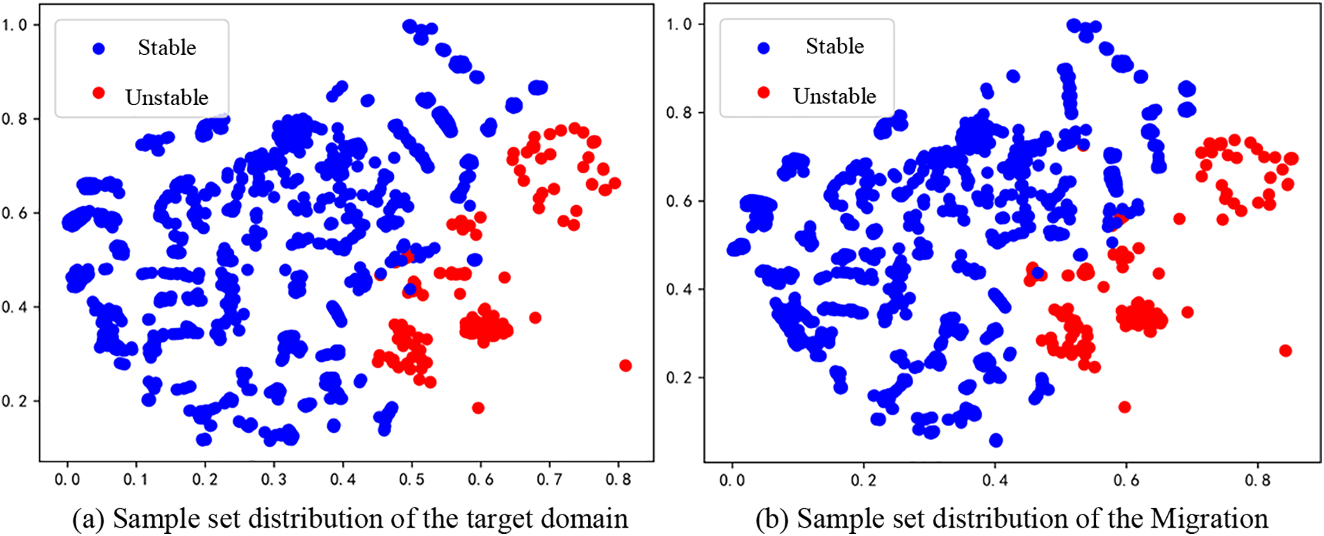
Figure 1: Comparison of sample set distribution before and after migration

4  Transient Stability Assessment Based on Improved XGBoost

4.1 Input Feature Selection

The selection and construction of input features directly impact the evaluation performance of the TSA model [24]. The existing research categorizes the transient stability feature sets into two types: the first type is based on expert knowledge, considering state variables that comprehensively reflect the dynamic characteristics of the system during transient processes. It utilizes combined features obtained through mathematical operations, but the calculations are complex and cannot guarantee real-time evaluation. The second type directly uses time-series measurements from PMUs as inputs, which can reduce subjectivity caused by human intervention and improve the computational speed of the algorithm.

This paper aims to construct a TSA model that can perform online analysis based on underlying measurement data. To ensure comprehensive coverage of transient information, the following electrical quantities are selected as initial input features: bus voltage magnitude, phase angle, generator rotor angle, angular velocity, active power, reactive power, active and reactive power of the AC transmission lines, active and reactive power of the load. All these electrical quantities can be directly obtained through PMUs [25].

4.2 Model Tag Construction

For the transient stability assessment (TSA) problem in power systems, it is typically classified as a binary classification problem [26]. This paper introduces a transient stability index (TSI) [27], which evaluates the power angle stability of the system after experiencing significant disturbances, as shown in Eq. (13).

TSI=360°−|Δδmax|360°+|Δδmax|(13)

where Δδmax represents the maximum angular difference in power angle between any two generators at any given time. When Δδmax is less than 360°, i.e., TSI is greater than 0, the system is in transient stability, and the sample is labeled as 0. Conversely, if the system is transiently unstable, with Δδmax exceeding 360°, the sample label is set as 1.

4.3 Model Evaluation Index

Accuracy is the most commonly used metric for evaluating the performance of machine learning models, but it cannot reflect the degree of attention paid to minority class samples. In practical applications, ignoring the judgment of unstable samples may cause large-scale cascading failures, resulting in more serious consequences than misjudging stable samples as unstable samples. Therefore, it is necessary to pay extra attention to the model’s ability to identify unstable samples, rather than using a single overall accuracy metric to measure the performance of the transient voltage stability assessment model. The confusion matrix for transient power angle stability evaluation is defined as shown in Table 1.

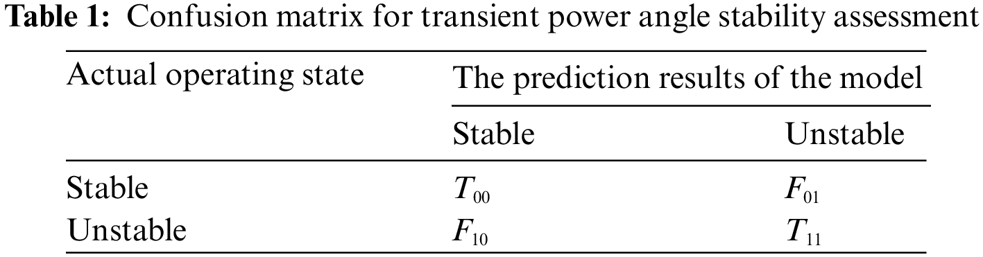
In Table 1, T00, T11, F01, F10 respectively represent the number of samples correctly predicted as stable, correctly predicted as unstable, stable samples incorrectly predicted as unstable, and unstable samples predicted as stable. Based on this, the model performance evaluation metrics accuracy, misjudgment rate, and recall are defined as shown in Eqs. (14)–(16).

ACC=T00+T11T00+F01+F10+T11(14)

MIS=F10T00+F01+F10+T11(15)

REC=T11F01+F10(16)

4.4 Evaluation Process

The TSA process based on improved XGBoost proposed in this paper consists of two parts, namely offline training and online evaluation, as shown in Fig. 2.

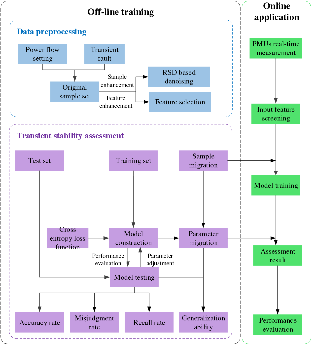
Figure 2: Transient stability assessment process

Firstly, the raw dataset reflecting different power flow operating modes and fault conditions is generated through time-domain simulation software, and the transient electrical quantities in 2.1 are extracted as input features. The dataset is randomly divided into a training set and a test set, with the training set used to construct the XGBoost model, and the test set used to evaluate the model’s performance and adjust the model parameters based on the test results. At the same time, the original sample set and model parameters are transferred to the target domain, and the model’s generalization ability is validated on the test set in the target domain. In online applications, the transient power angle stability of the system can be quickly determined by feature selection based on real-time measurement information provided by PMUs.

5  Analysis of Algorithms

5.1 Simulation Conditions

To validate the effectiveness of the proposed method, the commonly used IEEE 39-bus system is adopted as a case study for transient stability analysis. The simulation platform used is PSASP. Five different load levels are considered: 80%, 90%, 100%, 110%, and 120%. The fault type is three-phase short circuit, occurring at 1%, 50%, and 99% of each line, with fault durations of 0.1, 0.15, and 0.2 s. Samples are labeled as stable if they remain stable during the fault, otherwise they are labeled as unstable. A total of 12,000 samples are obtained through simulations, with 2,476 unstable samples and 9,524 stable samples. 70% of the samples are randomly selected as the training set, while the remaining 30% are used as the testing set.

5.2 Data Preprocessing

The time series extracted by PMU often contains outliers and outliers. In this paper, the gradient detection method is adopted and the sliding time window size is set to 5, so that sample points with the smallest gradient change can be screened out in each segment to avoid the interference of extreme data on sample prediction, as shown in Fig. 3.

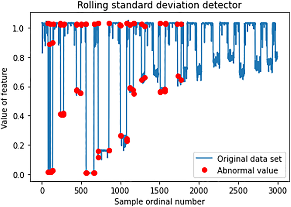
Figure 3: Sample denoising based on gradient detection

In terms of features, the first step is to select the number of feature subsets based on the incremental method and cross-validation. As shown in Fig. 4, when the number of features is 132, the model achieves the optimal evaluation accuracy of 0.987. This ensures that the model covers the essential transient information while minimizing the feature dimension as much as possible to improve computational efficiency.

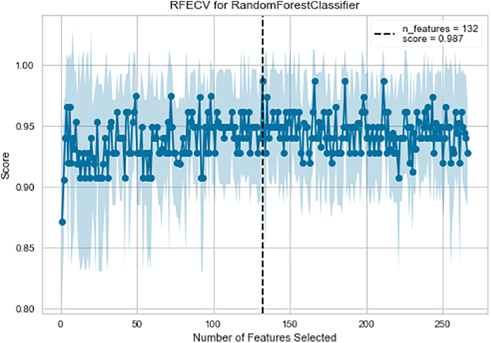
Figure 4: Sample denoising based on gradient detection

Next, the contribution of each input feature is ranked based on the SHAP principle, as shown in Fig. 5. G represents the generator, B represents the bus, L represents the load, AP represents the active power, PA represents the power angle, and VA represents the voltage amplitude. As shown in the figure, features such as the active power of the generator, power angle difference, bus voltage, and active power of the load have a significant impact on the transient stability of the system. Finally, 132-dimensional variables before contribution are selected as inputs to the data-driven model.

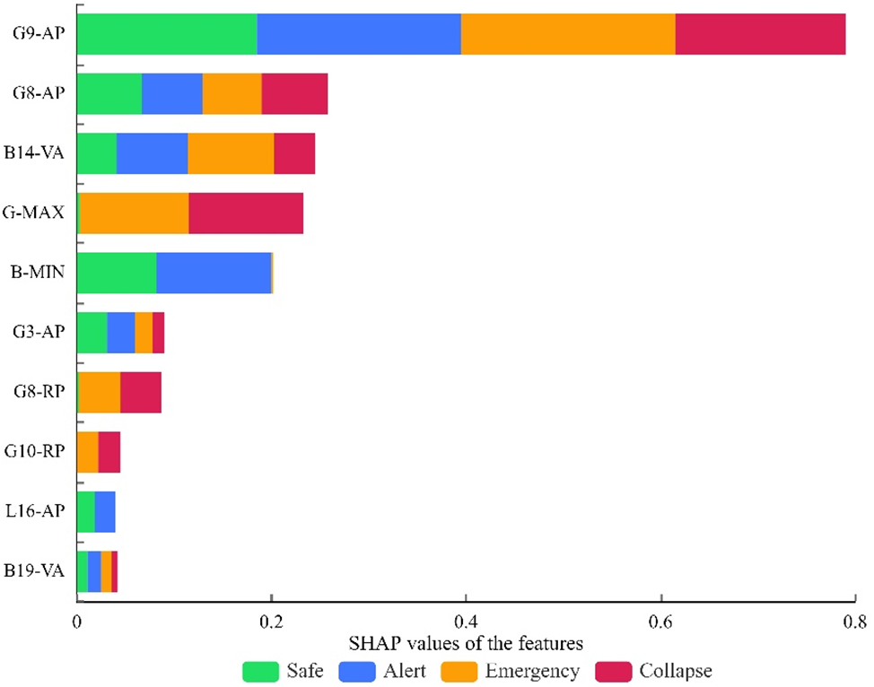
Figure 5: Feature contribution degree based on SHAP

5.3 Model Performance Comparison

To verify the impact of the proposed sample-feature enhancement strategy on model evaluation results, a comparison was made between the performance of the model using the original data, data denoised using only rolling standard deviation, data with only feature reduction, data denoised using the soft threshold method [12], and the proposed method in this paper, as shown in Table 2.

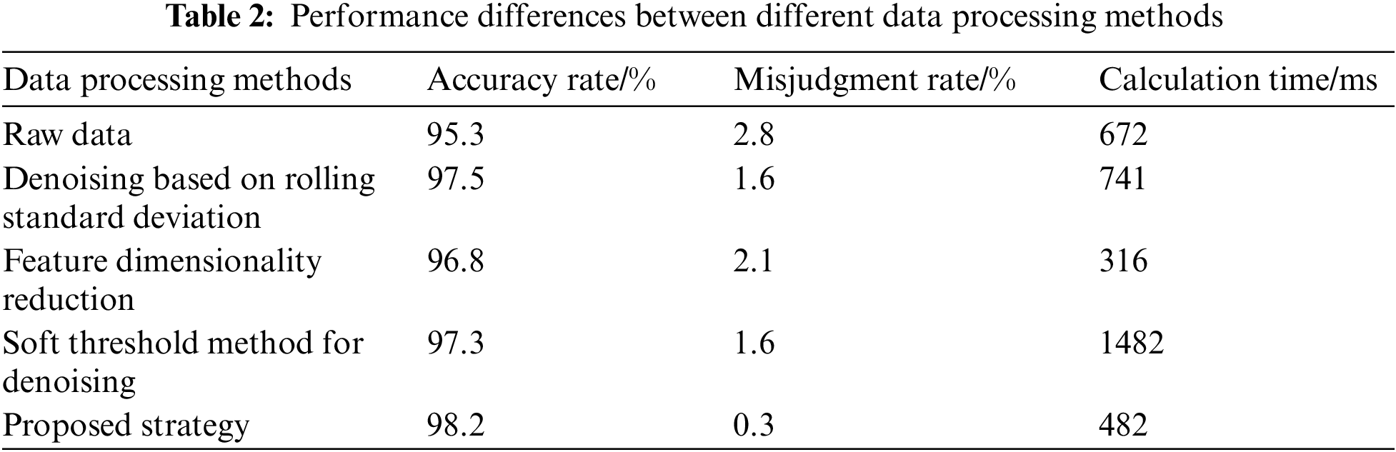
According to Table 2, the denoising method based on rolling standard deviation detection significantly improved the accuracy of the model and reduced the misjudgment rate by 1.2%. Although the soft threshold denoising method had a similar prediction accuracy, it greatly increased the evaluation time due to the need to calculate attention weights. The data enhancement strategy proposed in this paper comprehensively considered the feature dimension and noise impact, which improved the accuracy by 2.9% and reduced the computation time by 28.2%.

To compare the differences between commonly used machine learning models and the proposed method, this study selects artificial neural network (ANN), multi-layer perceptron (MLP), random forest (RF), convolutional neural networks (CNN), generative adversarial network (GAN), long short-term memory network (LSTM), and support vector machine (SVM) as benchmarks for transient stability assessment. The training and testing samples used are consistent across all models. The evaluation results of each model on the testing set are presented in Table 3.

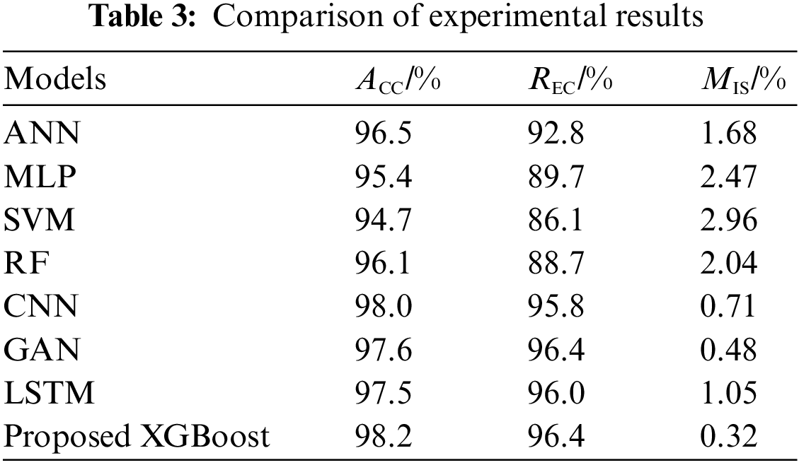
According to Table 3, it can be seen that XGBoost has the highest evaluation accuracy, reaching 98.2%. ANN and MLP, as neural networks, also achieve relatively ideal results after parameter optimization, but their accuracy is still 1.7% lower than that of XGBoost mentioned. SVM and RF, as shallow machine learning models, have lower accuracy, especially in terms of recall rate and misjudgment rate. CNN and GAN, after tuning and optimization, have an accuracy rate close to 98%, but there is still a higher probability of failing to detect faults. Overall, the XGBoost mentioned in this paper still has the highest recall rate, and the misjudgment rate can be reduced to 0.32%, which may simultaneously ensure the precision and recall of unstable samples.

5.4 Migration Effect Analysis

5.4.1 Migration under Topology Change

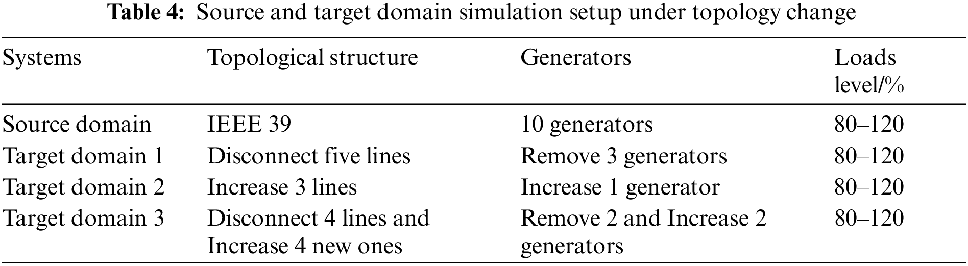
For the IEEE 39-bus system, in order to enhance the adaptability to changes in the system structure after line faults or emergency controls, modifications were made to its topology and operation. Three additional target scenarios were introduced, and their topology changes and simulation settings are shown in Table 4. For different topology structures, the sample migration method proposed in Section 3.3 was used to generate 3,000 training samples and 1,200 testing samples. The performance effects of pre-migration samples, fine-tuning of the sample set, and the sample-model migration method proposed in this paper were compared, and the test results are shown in Table 5.

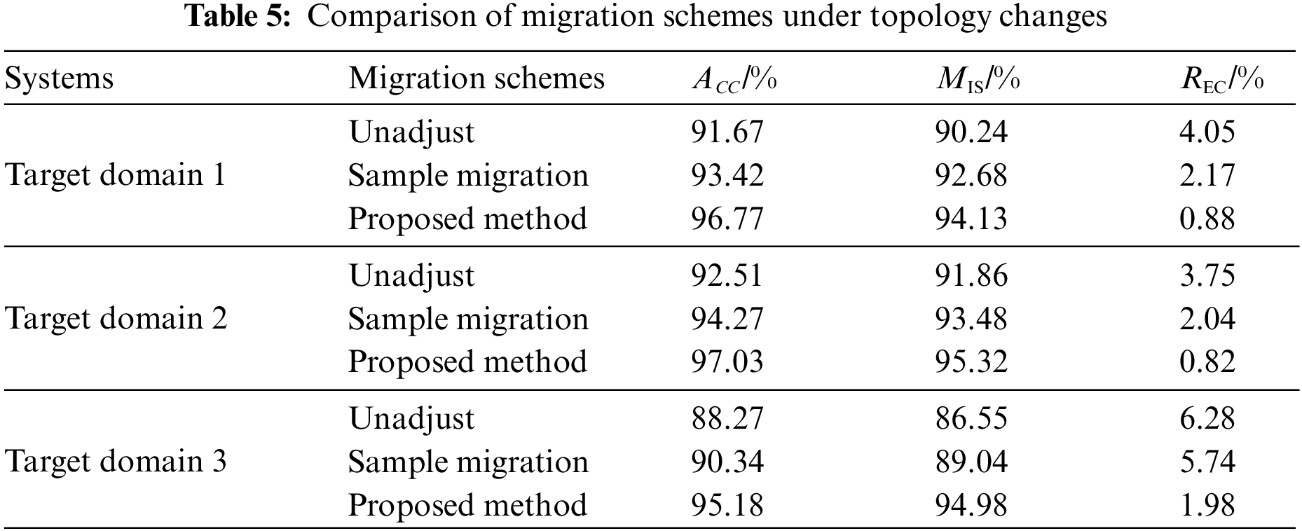
From Table 5, it can be seen that due to significant changes in the sample distribution of the target domain after topology changes, the performance of the model significantly decreases when directly evaluating it with the model before topology changes. When only using the sample migration method, there is some improvement, but the misjudgment rate and omission rate remain at a high level. Moreover, for target domain 3, which experiences significant changes in topology, all indicators show a noticeable decline, making it unsuitable for online applications. However, by using the method proposed in this paper, compared to before migration, there is a significant improvement of 6.91% and 8.43% in the highest achieved recall rate and precision rate for domains ACC and MIS, respectively. Additionally, there is a 4.3% reduction in REC. This method significantly reduces the probability of failing to detect instability in real power systems in a timely manner, achieving adaptive evaluation of transient stability under topology changes.

5.4.2 Migration under Changing Operating Conditions

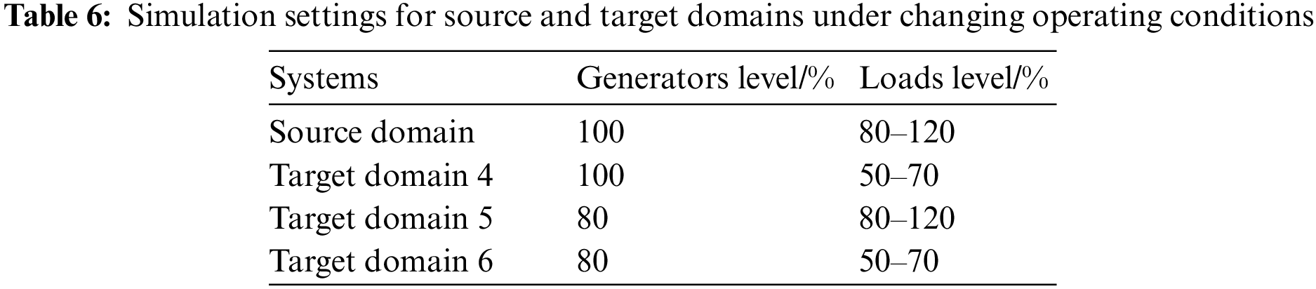
In order to enhance the adaptability under multiple operating conditions, we set up variations in generator and load levels under the same topological structure conditions, as shown in Table 6. For each operating condition, we generated 3,000 training samples and 1,200 testing samples. We compared the performance of pre-migration, fine-tuning on the sample set, and the sample-model migration method proposed in this paper, and the test results are shown in Table 7.

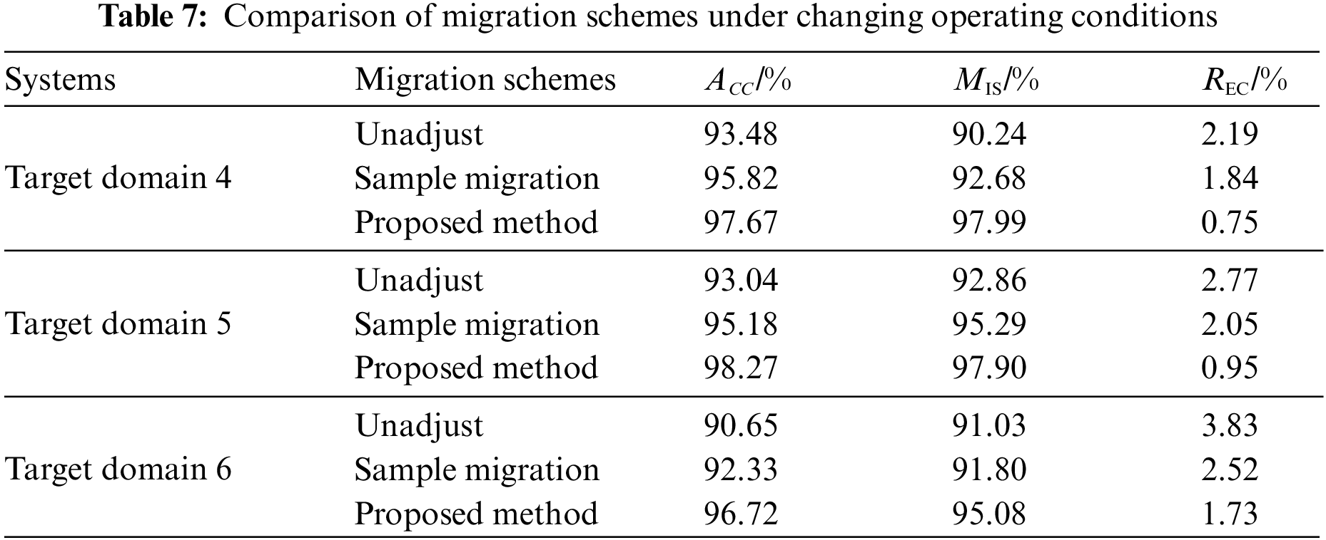
According to Table 7, it can be seen that the impact of changes in operating conditions on model evaluation is weaker than that of changes in topology. The model still maintains an accuracy of 93.48% without adjustment. However, when both the generator and load level are changed simultaneously, the accuracy drops to nearly 90%. The method proposed in this paper can adapt to various extreme changes, compared to single sample transfer, and has strong generalization ability, which can ensure real-time response of online evaluation.

5.4.3 Migration Time Comparison

For a power system with a new topology or operating conditions, traditional methods generate a large number of labeled samples by re-simulating and then retrain a new model based on these samples. This process usually takes a lot of time. The comparison of the time consumption between the proposed method and the retraining process is shown in Table 8.

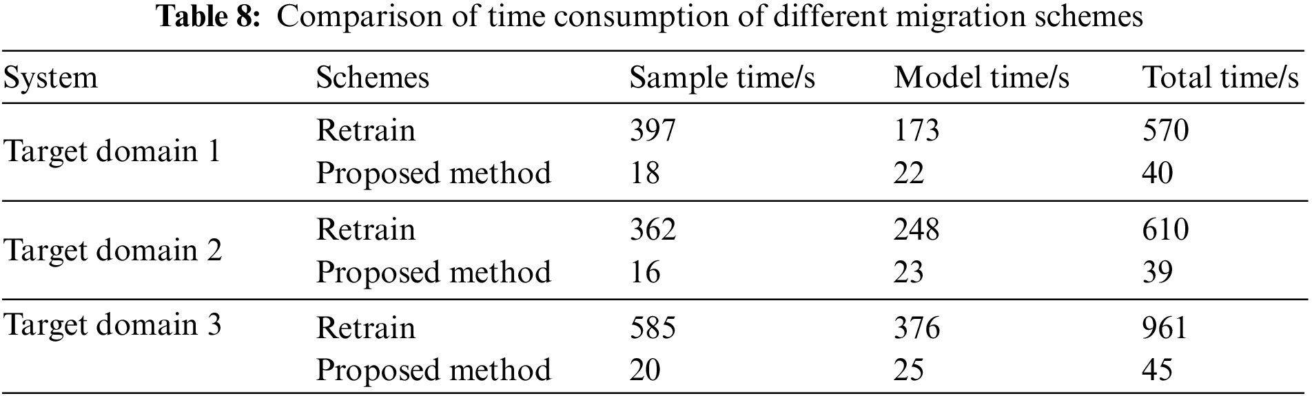
The test results indicate that the proposed transfer learning method is significantly faster in terms of training speed compared to retraining. For unidirectional adjustments in the topology structure, the model’s update efficiency is improved by 14–15 times. For complex structural adjustments, the efficiency improvement can exceed 20 times. This substantial reduction in online evaluation time meets the requirements for timeliness.

6  Conclusions

The paper proposes an improved XGBoost-based method for transient stability assessment, aiming to address the issues of low accuracy and insufficient generalization ability in the existing power system transient stability evaluation. The proposed method is tested and validated on the IEEE 39-bus system, and the conclusions are as follows:

1) The proposed sample-feature enhancement strategy reduces extreme data caused by noise interference, resulting in a 2.9% increase in accuracy and a 28.2% improvement in computational efficiency compared to existing algorithms.

2) The proposed transient stability assessment algorithm improves the loss function based on cross-entropy to guide the model’s attention towards unstable samples of the minority class. Compared to existing machine learning methods, the accuracy is improved to 98.2%, and the misjudgment rate is significantly reduced to below 0.35%.

3) The proposed transfer learning method based on model parameter and sample enhancement demonstrates strong adaptability to changes in topology structure and operating conditions. It achieves a 6.9% and 3.3% increase in accuracy respectively when facing changes in topology structure and operating conditions. Moreover, the computational efficiency is improved by more than 14 times, meeting the requirements for online evaluation.

The TSA method proposed in this paper qualitatively discriminates stable and unstable samples. In future work, the stability and instability margins will be further quantified, and faulted lines under transient instability conditions will be accurately identified using fault location techniques, providing a basis for power grid dispatchers to investigate potential hidden dangers in the system. Additionally, the offline sample set used for transient stability assessment is mostly generated through time-domain simulation methods. Future research will focus on the sample level to make the simulated samples more closely resemble actual measured data, thereby improving the evaluation model.

Acknowledgement: None.

Funding Statement: This work is supported by the State Grid Shanxi Electric Power Company Technology Project (52053023000B).

Author Contributions: The authors confirm contribution to the paper as follows: study conception and design: Ying Qu and Jinhao Wang; data collection: Xueting Cheng and Jie Hao; analysis and interpretation of results: Weiru Wang; draft manuscript preparation: Zhewen Niu. All authors reviewed the results and approved the final version of the manuscript.

Availability of Data and Materials: The datasets used and/or analysed during the current study are available from the corresponding author on reasonable request.

Conflicts of Interest: The authors declare that they have no conflicts of interest to report regarding the present study.

References

1. Zhu, S., Liu, K. Q., Qin, L., Li, G., Hu, X. L. et al. (2017). Analysis of transient stability of power electronics dominated power system: An overview. Proceedings of the CSEE, 37(14), 3948–3962 (In Chinese). [Google Scholar]

2. Karbalaei, F., Shabani, H. R., Abbasi, S. (2023). Pre- and post-disturbance transient stability assessment using intelligent systems via quick estimating of the critical clearing time. International Journal of Emerging Electric Power Systems, 24(3), 341–349. https://doi.org/10.1515/ijeeps-2021-0386 [Google Scholar] [CrossRef]

3. Zhang, Y., Han, X. Q., Zhang, C., Qu, Y., Liu, Y. et al. (2023). Parallel integrated model-driven and data-driven online transient stability assessment method for power system. Energy Engineering, 120(11), 2585–2609. https://doi.org/10.32604/ee.2023.026816 [Google Scholar] [CrossRef]

4. Shrivastava, D. R., Siddiqui, S. A., Verma, K., Singh, S., Alotaibi, M. A. et al. (2023). Data-driven unified scheme to enhance the stability of solar energy integrated power system in real-time. IEEE Access, 11, 118443–118461. https://doi.org/10.1109/ACCESS.2023.3325195 [Google Scholar] [CrossRef]

5. Chen, Q. F., Lin, N., Wang, H. Y. (2021). Transient stability assessment model with parallel structure and data augmentation. International Transactions on Electrical Energy Systems, 31(5), e12872. [Google Scholar]

6. Li, M., Lei, M., Zhou, T., Li, Y. L., Xiao, Y. et al. (2021). A deep forest-based transient stability assessment method for power systems. Electrical Measurement and Instrumentation, 58(2), 53–58. [Google Scholar]

7. Tian, F., Zhou, X. X., Yu, Z. H. (2017). Transient stability assessment of power system based on support vector machine integrated classification model and key sample set. Power System Protection and Control, 45(22), 1–8. [Google Scholar]

8. Sun, L. X., Bai, J. T., Zhou, Z. Y. (2020). Transient stability assessment of power system based on bidirectional long- and short-term memory network. Automation of Electric Power Systems, 44(13), 64–72. [Google Scholar]

9. Li, Y., Yang, Z. (2017). Application of EOS-ELM with binary jaya-based feature selection to real-time transient stability assessment using PMU data. IEEE Access, 5, 23092–23101. https://doi.org/10.1109/ACCESS.2017.2765626 [Google Scholar] [CrossRef]

10. Liu, S. C., Liu, S. K., Zhang, L. (2022). Robust transient stability assessment of power systems considering sample imbalance. Smart Power, 50(7), 16–22+73 (In Chinese). [Google Scholar]

11. Liu, F., Wang, X. D., Li, T., Huang, M. Z., Hu, T. et al. (2023). An automated and interpretable machine learning scheme for power system transient stability assessment. Energies, 16(4), 1956–1972. [Google Scholar]

12. Lu, J. L., Guo, L. Y. (2021). Transient stability assessment of power system based on improved deep residual shrinkage network. Journal of Electrical Engineering Technology, 36(11), 2233–2244. [Google Scholar]

13. Wen, T., Zhang, M., Wang, H. Y. (2022). Transient stability evaluation model based on stacked sparse noise-reducing self-encoder. Power Engineering Technology, 41(1), 207–212. [Google Scholar]

14. Yang, D. S., Ji, M. J., Zhou, B. W. (2021). A transient stability assessment method for power systems based on dual generator generative adversarial networks. Power System Technology, 45(8), 2934–2945. [Google Scholar]

15. Zhou, T., Yang, J., Zhou, Q. M. (2019). A transient stability assessment method for power systems based on improved LightGBM. Power System Technology, 43(6), 1931–1940. [Google Scholar]

16. Li, Y., Zhang, S., Li, Y., Cao, J., Jia, S. (2023). PMU measurements-based short-term voltage stability assessment of power systems via deep transfer learning. IEEE Transactions on Instrumentation and Measurement, 72, 1–11. [Google Scholar]

17. Lu, J. L., Guo, L. Y. (2021). Power system transient stability assessment based on improved deep residual shrinkage network. Transactions of China Electrotechnical Society, 36(11), 2233–2244. [Google Scholar]

18. Wang, B., Fang, B. W., Wang, Y. J., Liu, H. S., Liu, Y. L. (2016). Power system transient stability assessment based on big data and the core vector machine. IEEE Transactions on Smart Grid, 7(5), 2561–2570. https://doi.org/10.1109/TSG.2016.2549063 [Google Scholar] [CrossRef]

19. Zhao, D. M., Xie, J. K., Du, Z. H., Wei, Z. Q., Tian, S. F. et al. (2023). Transient feature selection and two-stage stability assessment of wind-fire system based on uniform information coefficient and Wasserstein-generative adversarial network. Electric Power Automation Equipment, 43(4), 106–113. [Google Scholar]

20. Zhang, F., Li, X. Y., Xu, W. T., He, L., Jing, Y. Q. (2012). An overlapping probability based feature selection method for evaluation of transient voltage stability. Power System Technology, 36(6), 116–121. [Google Scholar]

21. Wu, C. M., Ren, J. H. (2021). Power system transient stability assessment method based on XGBoost-EE. Electric Power Automation Equipment, 41(2), 138–143. [Google Scholar]

22. Peng, B. (2022). Research on operation stability evaluation of industrial automation system based on improved deep learning. International Journal of Manufacturing Technology and Management, 36(2–4), 141–153. [Google Scholar]

23. Du, Y. X., Hu, Z. J., Wang, F. Z. (2021). A hierarchical power system transient stability assessment method considering sample imbalance. Energy Reports, 7, 224–232. https://doi.org/10.1016/j.egyr.2021.08.052 [Google Scholar] [CrossRef]

24. Gu, X. P., Li, Y., Jia, J. H. (2015). Feature selection for transient stability assessment based on kernelized fuzzy rough sets and memetic algorithm. International Journal of Electrical Power and Energy Systems, 64, 664–670. https://doi.org/10.1016/j.ijepes.2014.07.070 [Google Scholar] [CrossRef]

25. Behdadnia, T., Yaslan, Y., Genc, I., A new method of decision tree based transient stability assessment using hybrid simulation for real-time PMU measurements. IET Generation, Transmission and Distribution, 15(4), 678–693. https://doi.org/10.1049/gtd2.v15.4 [Google Scholar] [CrossRef]

26. Wang, G. Z., Guo, J. B., Ma, S. C., Zhang, X., Guo, Q. L. et al. (2023). Data-driven transient stability assessment using sparse PMU sampling and online self-check function. CSEE Journal of Power and Energy Systems, 9(3), 910–920. [Google Scholar]

27. Liu, X. Z., Min, H., Chen, L., Zhang, X. H., Feng, C. Y. (2021). Data-driven transient stability assessment based on kernel regression and distance metric learning. Journal of Modern Power Systems and Clean Energy, 9(1), 27–36. https://doi.org/10.35833/MPCE.2019.000581 [Google Scholar] [CrossRef]