Research on Demand Response Potential of Adjustable Loads in Demand Response Scenarios

1  Introduction

The proposal of the dual carbon target has put forward higher requirements for the development of new energy and the transformation of energy [1]. With the massive integration of new energy, on the one hand, the gradual increase in the proportion of installed capacity and grid connection of new energy generation greatly weakens the flexible regulation ability of the power generation side [2]; on the other hand, the uncertainty of new energy output poses higher requirements for the implementation of system regulation. Relying solely on adjustable resources on the power generation side to maintain the stability of the power system is no longer sufficient [3]. Therefore, invoking demand-side resources has become an effective measure to solve the above problems [4]. In January 2022, the National Development and Reform Commission and the National Energy Administration issued the “Opinions on Improving the System, Mechanism, and Policy Measures for Energy Green and Low Carbon Transformation” [5] and the “14th Five Year Plan for Modern Energy System” [6], which pointed out: expand the implementation scope of electricity demand, explore demand side resources through various methods and encourage electricity users to participate in demand response (DR); carry out aggregation of various loads such as industrial loads, air conditioning loads and new energy vehicle loads; Actively promote the participation of emerging market entities such as load aggregators (LA) in the DR market. In participating in DR, LA will provide various incentive policies for users to choose and guide them to participate in DR.

DR guides users to change their electricity consumption behaviors through price or incentive signals so that electricity consumption is reduced/increased, which promotes the balance of supply and demand. When there are peaks or valleys in the the power grid operation, the DR demand side will determine the DR quantity and release relevant information to the DR market; The DR supply side shall bid based on its adjustable load of DR and obtain profits. Wherein, evaluating the demand response potential (DRP) of various adjustable loads is significant for formulating incentive policies.

For DRP evaluation, the initial research mainly focused on qualitative evaluation. In reference [7], the method of questionnaire survey was used to obtain survey results, and the main influencing factors of a user participating in DR were analyzed from the results. In reference [8], the internal relationship between energy usage and DR was analyzed through a survey questionnaire. However, questionnaire surveys have the problem of high workload and long time consumption. Afterward, some scholars proposed that the relationship between factors and DRP was analyzed directly. In reference [9], the functional relationship between DRP and temperature, and time was established based on the least squares method and fitted it. In reference [10], the method of using load rate to represent DRP was proposed and evaluated DRP based on the maximum load and average load rate of various users on typical days. In reference [11], the models of various loads, such as electric vehicles and temperature-controlled loads were established, and the DRP of each load was obtained based on the collected information. On this basis, feature mapping into DRP evaluation was introduced gradually. In reference [12], the DRP evaluation model based on deep adaptive neural networks was proposed, which evaluated the DRP by analyzing the similarity of their load characteristics. In reference [13], the DRP evaluation model based on a genetic algorithm sequence quadratic programming algorithm was established by analyzing characteristics of users’ energy consumption behavior and the proportion of electricity load. In reference [14], the user load was decomposed and features were extracted, by which a DRP evaluation model based on Gaussian process regression was established. Although the above research introduces feature mapping into DPR, it is difficult to represent the user’s DPR using DR power alone fully and accurately.

Moreover, due to the importance of information security and personal privacy, users have very strict protection measures for loading information. In reference [15], a revocable and lightweight blockchain access control for smart electronic products is proposed which achieves partial hiding of access information and forward and backward data security; In reference [16], a dynamic multi-keyword ranking search scheme is proposed based on encrypted cloud data privacy protection to ensure the security of cloud data sharing; In reference [17], a lightweight mutual authentication protocol is proposed based on blockchain technology which ensures the security and privacy of drone data. The above literature indicates that the protection of user data is getting better and better currently. Therefore, the difficulty of obtaining adjustable load data for LA increases and the amount of data obtained is insufficient, resulting in deviations in DPR evaluation and DR plan formulation for DRP.

In summary, the above research has the following shortcomings: (1) There is limited research on the characteristic relationship between influencing factors and DRP and there is a lack of data on adjustable loads, which affects the prediction and calculation of DRP; (2) In the process of DRP evaluation, only considering DR power without considering other factors in the DR cannot comprehensively and accurately evaluate DRP of adjustable loads; (3) There is no basis for developing different adjustable load participation plans for different DR scenarios, resulting in poor DR effectiveness.

Based on this, the article proposes a demand response potential feature extraction and prediction model based on data mining and a DRP evaluation model based on subjective and objective weight analysis. The innovation is reflected in: (1) By analyzing the DR process and DR behavior, the characteristics that affect DR are obtained, solving the problem of only using DR power to represent DRP. (2) Utilize the theory of data similarity and the relationship between various DR features, as well as between various DR features and DRP are mined fully to improve the efficiency and accuracy of model prediction. (3) The various DR feature prediction data obtained from the above prediction models represent different demand response scenarios and adjustable loads and a DRP evaluation model for subjective and objective weight allocation is established to calculate the DRP of different adjustable loads in different DR scenarios, overcoming the defect of poor demand response caused by unified calling.

2  Characteristics of DR

Because changing one’s electricity consumption behavior to achieve DR is a process rather than an instant, it is not comprehensive to solely reflect the adjustable load DRP through DR power [18]. Therefore, considering the factors of user participation in DR, the article comprehensively evaluates the DRP of adjustable load by characterizing the characteristics of the DR process and DR behavior.

2.1 The Process of DR

When users participate in DR: adjustable loads are initially in the normal electricity consumption process. When receiving the DR signal, users change their electricity consumption behavior and use electricity according to the response signal, which is a response reaction process; After meeting DR requirements, adjustable loads will operate in a new stable state, which is a continuous response process; After receiving the signal indicating the end of DR, users resume their electricity consumption behavior to normal electricity consumption, which is a response recovery process. As shown in Fig. 1.

Figure 1: The process of DR

Wherein, the characteristics that characterize the DR process are defined as follows:

(1) Initial output Pini: it represents the adjustable load that the user does not participate in DR.

(2) Min/Max output Pmin/max: it represents the maximum/minimum adjustable load that the user can participate in DR and the maximum adjustable load is used for upward adjustment; The minimum adjustable load is used for downward adjustment.

(3) Adjustment amplitude A: it represents the maximum ability of the user to participate in the up/down adjustment of DR, which is the difference between the initial output and the Min/Max output.

(4) Response time TR: it represents the response efficiency of the user to participate in DR. The shorter the response time, the better the response effect.

(5) Response duration TD: it represents the sustained stability of the user to participate in DR. The longer the duration, the better the response stability.

(6) Climbing rate R: it reflects the relationship between response regulation ability and response time. It is defined as the ratio of regulation amplitude to response time.

(7) Regulation ability D: it is defined as the user’s ability to participate in both upward and downward regulation of DR.

Because the DR demand side has strict requirements for the response time, efficiency, and regulation ability of the DR supply side (such as adjustable load). The closer the DR on the DR supply side is to the requirements of the DR supply side, the better the DR effect and the higher the DPR. The characteristics that characterize the DR process in the above models can serve as indicators of adjustable load DPR, representing the impact of the DR process on DPR.

2.2 The Behavior of DR

When a user is not involved in DR, the electricity load is the baseline load; when participating in DR, the user changes electricity consumption behavior, so that the load curve will change. At this time, the load is the actual load and the difference between the baseline load and the actual load is the DR quantity of the load. Therefore, DR quantity is related to both the baseline load and the actual load, which is shown in Fig. 2.

Figure 2: DR behavior curve

The solid line in Fig. 2 represents the baseline load curve and the dashed line represents the actual load curve. The difference between the solid line and the dashed line is DR quantity. As shown in the figure, when the baseline load is at its peak period, the load participating in DR shows a DRP of decrease; When the baseline load is in a valley period, the load participating in DR shows a DRP of upregulation.

Because DR quantity is an important factor reflecting DPR, which is the difference between baseline load and actual load is DR quantity, its result directly affects the economic benefits of DR demand side and supply side. Therefore, using baseline load and actual load as DPR indicators represents the impact of DR behavior on DPR.

In addition to the relevant characteristics of the DR process and DR behavior, the article introduces the concept of response capacity ratio, which is specifically represented as follows:

Rcr=Rk,iCk,i(1)

where Rk,i denotes the response load capacity of the user k during the period i; Ck,i denotes the actual load capacity of the user k during the period i. This physical quantity represents the adjustable capacity of an adjustable load and the smaller its value, the stronger its adjustability, reflecting the smaller proportion of the response quantity in the electricity consumption.

So, the characteristics that characterize DR behavior are as follows:

(1) Baseline load Bk,i: it reflects the load situation when users did not participate in DR.

(2) Actual load Ck,i: it reflects the load situation when users participate in DR.

(3) Response load Rk,i: it is defined as the DR amount of adjustable load, which is the difference between baseline load and actual load.

(4) Response capacity ratio Rcr: it reflects the difficulty of load regulation when users participate in DR, which is the ratio of response load to actual load.

3  DR Feature Extraction and Prediction Based on Data Mining

Data mining is an interdisciplinary field. Hand et al. provided a general definition: analyze datasets, explore the relationships between datasets, and express them in a novel and understandable way. Afterward, Tan et al. defined data mining as a method of extracting information hidden in the data. From those, it can be seen that data mining tasks include exploratory data analysis, descriptive data modeling, predictive data analysis, and so on. Wherein, temporal data mining is a method of discovering information and knowledge from time series data [19]. As shown in reference [20], data mining is used to extract data features that affect load. Load prediction is performed based on the extracted features to improve the efficiency and accuracy of model prediction. Therefore, the article adopts the data mining model to extract features and predict the extracted feature data. In the process of extracting and predicting DR features, differences in data can affect the accuracy of the results. There are two methods: continuous time series in periods and different date time series in the same period [21]. The model established based on continuous time data has more complex features and poor regularity; however, the data from the same period can better reflect the electricity usage habits of users during this period with more obvious and regular characteristics. Therefore, the article uses simultaneous data as input for the data mining model.

Using the historical date data of the same period mentioned above, the DR feature data of each response day are obtained through similar day clustering, temporal decomposition, redundancy processing, and data prediction. The specific flowchart is shown in Fig. 3.

Figure 3: Feature extraction and prediction flowchart based on data mining

Firstly, the article uses the Affinity Propagation (AP) algorithm for similar day clustering to improve the correlation between historical data and prediction results; Secondly, the Ensemble Empirical Mode Decomposition (EEMD) algorithm [22] is selected to decompose the data of the same segment sequence, making the data features singular; Thirdly, Pearson Correlation Coefficient (PCC) method is chosen to analyze the redundancy between feature quantities, ensuring that the input data volume and feature dimensions of the model prediction are reduced while fully expressing DRP; Finally, based on the extracted features mentioned above, corresponding historical data is obtained. A prediction model based on Gaussian Process Regression (GPR) is established to predict the extracted DR features, which are used as user response day DRP evaluation data.

3.1 Similar Day Clustering Based on AP

Due to the influence of time factors on electricity load, extracting dates with similar day types (such as workdays or weekends) can effectively improve the accuracy of load forecasting and calculation models. The article uses an AP clustering algorithm to determine historical dates similar to response dates. The advantage of AP algorithm clustering is that there is no need to determine the number of clusters; there is no sensitivity to the initial value of the data; there is no requirement for the symmetry of the initial similarity matrix data. The specific steps for clustering are as follows:

(1) Construct a cluster indicator set. The article uses seven electricity consumption indicators that can reflect the daily load usage, as shown in Table 1. Wherein, load rate is the ratio of average load to maximum load, minimum load rate is the ratio of minimum load to maximum load and peak valley difference rate is the ratio of peak valley difference to maximum load.

(2) The above seven features form a set of clustering indicators for each user, which serve as inputs to the AP clustering algorithm and ultimately obtain clustering results for similar days.

3.2 Load Timing Decomposition Based on EEMD

Based on the above clustering analysis results, adjustable loads of similar days before the response day are decomposed. The article adopts the EEMD algorithm. This algorithm utilizes Gaussian white noise, which has a statistical characteristic of uniform frequency distribution. By adding different white noise of the same amplitude each time, the extreme point characteristics of the signal are changed. Then, the corresponding IMF obtained from multiple EMDs is overall averaged to offset added white noise, which effectively suppresses the generation of modal aliasing. The steps are as follows: (1) add Gaussian white noise to the original sequence and set the average amplitude of the sequence to 0; (2) use the EMD algorithm to decompose sequences with added white noise; (3) repeat the above two steps to obtain different modulus functions until the EMD termination condition is met; (4) average sets of modular functions to cancel out the added white noise and obtain the final decomposition result.

Through the EEMD algorithm, the actual load curve and response load are decomposed into different characteristic components. Each curve represents a characteristic of the actual load/response load. The characteristics of the response load amount and actual load are represented as:

Rk,i=[r1,r2,…rm](2)

Ck,i=[c1,c2,…cm](3)

where Rk,i denotes the response load capacity of the user k during the period i; Ck,i denotes the actual load capacity of the user k during the period i; m is the characteristic number of decomposition; rm is the feature quantity of the item m after response load decomposition; cm is the feature quantity of the item m after actual load decomposition.

3.3 Redundancy Analysis Based on PCC

Based on the above analysis, the characteristics of the DR process and DR behavior, as well as the response capacity ratio will be represented as a set S, as follows:

F=[Pini,Pmin/max,A,TR,TD,D,r1,…,rm,c1,…,cm](4)

where Pini denotes the initial output of load; Pmin/max denotes the minimum/maximum output; A denotes the adjustment amplitude which is the difference between the initial output and the minimum/maximum output; TR denotes the response time of DR; TD denotes the duration of DR; D denotes the adjustable ability, with 1 for up-regulation and 0 for down-regulation; Rcr denotes the response capacity ratio.

Redundancy is the analysis of the correlation between features, to reduce the number of features and improve the prediction efficiency of the model while ensuring that there is not a significant loss of information. The article uses the PCC method to analyze the redundancy between features. Assume two characteristic variables-A={a1,a2,…,a96} and B={b1,b2,…,b96}. The correlation is expressed as:

Rc=∑i=196(ai−a¯)(bi−b¯)∑i=196(ai−a¯)2(bi−b¯)2(5)

where A and B denote two feature datasets; ai denotes the data value of the item i in feature A; bi denotes the data value of the item i in feature B; a¯ denotes the mean of data in feature A; b¯ denotes the mean of data in feature B.

By clustering, decomposition, and redundancy processing, DR features are extracted to form a DR feature set F.

3.4 Feature Prediction Based on GPR

To obtain the feature data of response day, the article takes the extracted similar daily historical data of each feature as input and constructs a response day prediction model to obtain the predicted data of each feature of response day. Predicting the various characteristics of response day can determine the adjustable load DRP of response day, which can provide data support for establishing a DRP assessment model for adjustable loads under DR scenarios on the response day.

Based on this, the article establishes a probability prediction model based on GPR for extracted features, to reduce the impact of result uncertainty while improving the prediction accuracy of the model. According to reference [23], a large amount of data follows a Gaussian distribution, so the article adopts the GPR algorithm. This algorithm has the following advantages: it has autonomous learning ability and can learn the mapping relationship between input and output; the output value of the model is the difference between observed values and different kernels have different functions; it can achieve online fitting, strong generalization ability, and few parameters. The specific process of the feature prediction model based on GPR is shown in Fig. 4.

Figure 4: Extracted feature prediction flowchart based on GPR

To analyze the performance of the model, the article selects two common mathematical quantities: Mean Absolute Error (MAE) and Root Mean Square Error (RMSE). The specific formula is as follows:

MAE=1n∑i=1n|y^i−yi|(6)

RMSE=1n∑i=1n|y^i−yi|2(7)

where y^i denotes the predicted value of the item i data in the test set; yi denotes the true value of the item i data in the test set; n denotes the predicted data volume.

In addition, there are mathematical quantities for evaluating interval distribution: interval coverage, and interval average bandwidth. The specific formulas are as follows:

PICP=1n∑i=1nε(i)

ε(i)={1,f∗∈[fdown∗,fup∗]0,f∗∉[fdown∗,fup∗](8)

where n denotes the predicted data volume, ε(i) denotes the variable used to determine whether the predicted data is within the confidence interval, 1 indicates it is within the confidence interval and 0 indicates it is not within the confidence interval; f∗ denotes the predicted data, fup∗ denotes the upper bound of the confidence interval and fdown∗ denotes the lower bound of confidence interval.

Relying on reliability solely may result in a wide prediction interval so that is a decrease in the practical application value of prediction. So, introduce the interval average bandwidth to measure prediction sensitivity. The formula is as follows:

PINAW=1nR∑i=1n(fup∗−fdown∗)(9)

where R denotes the range of changes in the actual value of DRP. The smaller the PINAW, the stronger the sensitivity of prediction.

The predicted values obtained from the GPR model form the response day DR feature set.

4  Calculation and Evaluation of DRP for Adjustable Load in DR Scenarios

DR is regulation and scheduling of diversified adjustable loads on the demand side: assist in the wind and solar consumption of new energy grid connection, promote peak shaving and valley filling of power grid operation, and achieve optimal resource allocation. For different purposes, DR has different scenarios, such as frequency modulation DR, Peak shaving DR, and so on. Different scenarios require different DR capabilities of loads due to different DR purposes. The DR features extracted above can comprehensively reflect the DRP of a certain DR response scenario or load. Therefore, the article utilizes extracted DR features to represent different DR scenarios and various adjustable loads.

4.1 Establishment of DR Scenarios

Based on the above analysis, the following will establish four DR scenarios: frequency modulation, peak shaving, valley filling, and new energy consumption to evaluate the DRP of adjustable loads.

(1) Frequency modulation DR scenario

Frequency modulation is a modulation method in which the instantaneous frequency of a carrier wave varies according to the desired signal transmission. This method requires that the delay of adjustable loads is 1 s, but does not require high DR volume, DR duration, and adjustment amplitude of loads [24]. When the system frequency difference is less than △f, loads are adjusted upwards to increase system frequency; When the system frequency difference is greater than △f, the load is adjusted downwards to reduce system frequency. The response power Pf and the model of response load CLf are represented as follows:

Pf(t)=−Kdc△f

{CL1f(t)=Q1f(t−1)−Pf⋅△t⋅ηupfQN1fCL2f(t)=Q2f(t−1)−Pf⋅△t⋅ηdownfQN2f(10)

where Kdc denotes the droop coefficient of DR, CL1f(t) and CL2f(t) denote DR quantities adjusted upwards and downwards, Q1f(t−1) and Q2f(t−1) denote load quantities at the previous moment of response to load, △t denotes the sampling interval time, ηupf and ηdownf denote DR efficiency adjusted upwards and downwards, QN1f and QN2f denote the total response loads adjusted upwards and downwards.

(2) Peak shaving/valley filling DR scenario

Peak shaving/valley filling DR scenario is a measure to adjust electricity loads. According to different electricity consumption patterns of users, arrange the electricity consumption time of various users in a reasonable and planned manner so that the peak load is reduced and the low load is increased, which achieves a balance between power generation and consumption. These scenarios require adjustable loads with a latency of seconds, a large load response, a longer response duration, and a larger adjustment amplitude [25]. The regulating ability of peak shaving is downward regulation. The regulating ability of valley filling is upward regulation. When the actual total load exceeds the peak load control target value Pconmax or the actual total load is less than the valley load control target value Pconmin, the model of response power Ppv and response load CLpv is represented as follows:

Ppv={Pac−Pconmaxpeak shavingPconmin−Pacvalley filling

{CL1pv(t)=Q1pv(t−1)−Ppv⋅△t⋅ηdownpvQN1pvCL2pv(t)=Q2pv(t−1)−Ppv⋅△t⋅ηuppvQN2pv(11)

where Pac denotes the actual total load, CL1pv(t) denotes the DR amount of peak shaving, CL2pv(t) denotes the DR amount of valley filling, Q1pv(t−1) denotes load amount at the previous moment of response load of peak shaving, Q2pv(t−1) denotes load amount at the previous moment of response load of valley filling, △t denotes the sampling interval time, η up f and ηdowopndenotes the DR efficiency of peak shaving, denotes the DR efficiency of valley filling adjustment, QN1pv denotes the total response load amount of upward adjustment, QN2pv denotes the total response load amount of downward adjustment.

(3) New energy consumption DR scenario

The installed capacity of new energy is increasing year by year, leading to enormous pressure on the system to consume new energy. The scenario of new energy consumption is when the power generation of new energy exceeds load consumption, some measures need to be taken to absorb the excess power generation of new energy. This service requires adjustable load latency at the minute level, large load response, long duration, and large adjustment amplitude [26]. The model of response power Pnec and response load CLnec is represented as follows:

Pnec=Pneg+PTP−PL

CLnec(t)=Qnec(t−1)−Pnec⋅△t⋅ηnecQNnec(12)

where Pneg denotes the total power generation of new energy, PTP denotes the thermal power generation, PL denotes the total power consumption of load, CLnec(t) denotes DR amount of new energy consumption, Qnec(t−1) denotes load amount at the previous moment of response load, △t denotes the sampling interval time, ηnec denotes the DR efficiency of new energy consumption, and QNnec denotes total response load amount of new energy consumption.

4.2 Various Adjustable Loads Participating in DR

There are various adjustable loads involved in DR, and each load has different electricity consumption patterns and DR behaviors. The following are analyses of electricity consumption patterns and DR characteristics: electric vehicles, air conditioning, industrial loads, residents loads, and energy storage.

(1) Electric vehicles

Electric vehicles are relatively flexible and adjustable loads, which can be seen as both transferable and interruptible loads. Electric vehicles have strong time characteristics, flexible response, relatively large response amount, and average response time [27]. However, one disadvantage of this type of load is that it may experience peak and low electricity consumption times and the response duration is poor.

(2) Air conditioning

The air conditioning loads (referred to here as commercial air conditioning) utilize the thermal energy storage characteristics of the building to ensure the comfortable indoor temperature needs of users during the regulation process, with minimal impact on users. The advantages of air conditioning load response are long response duration, stable response, and easy unified regulation [28]. The disadvantage is that response time is relatively slow, regulation ability is poor, and it is greatly affected by seasonal weather.

(3) Industrial loads

Industrial loads have well-equipped infrastructure and large power capacity. This type of load requires an equal increase/decrease in capacity within a certain scheduling period, so it can be considered a transferable load [29]. The disadvantage is that once the industrial load starts, it cannot be easily stopped, so adjustment ability is relatively poor.

(4) Residential loads

Residential electricity refers to the load used by households, including lighting, electric heating, etc. According to the distribution of load electricity consumption, the electricity consumption is mainly based on cooling load and heating load. The characteristic of this load is that the power is small and the peak value is small. The disadvantage is that the willingness and the uncertainty of the duration of DR are high.

(5) Energy storage

Energy storage is a final consideration for LA in participating in DR. The advantages of energy storage are fast response, low uncertainty in response, and free response duration. The disadvantage is limited storage capacity.

The specific representation of each load response characteristic is shown in Table 2 (note: the data comes from the load data of a certain location participating in DR response).

4.3 Establishment of DRP Evaluation System Based on Subjective and Objective Weights

The evaluation system is an entirety that is constituted by characteristics characterizing various aspects of the evaluation object. The DR features extracted above comprehensively demonstrate the DR effect of adjustable loads and DR scenarios. Therefore, the above-extracted features are used as evaluation indicators to construct a DRP evaluation system. By calculating and analyzing the weights of various evaluation indicators for adjustable loads and DR scenarios, the DRP is fully expressed.

The weight of evaluation indicators reflects the degree to which each indicator affects the evaluation results and their calculation results directly affect the rationality and accuracy of evaluation results. The article adopts the subjective and objective analysis method, combining the subjective weights determined by the Analytic Hierarchy Process (AHP) with the objective weights determined by CRITIC, to obtain the combined weights of the impact of each evaluation indicator on the DRP of evaluation results. This can not only reflect the influence of subjective will but also fully consider the objective connection between various indicator data. The details are as follows:

(1) Determination of Subjective Weights Based on Analytic Hierarchy Process

To reflect the influence of subjectivity in data selection, the article uses AHP for weighting. The steps are as follows [30]: construct a judgment matrix; consistency inspection; and the solution of subjective weights.

(2) Objective Weight Determination Based on CRITIC Weighting

To reflect the objective connection between data, the article adopts the CRITIC method for objective weighting. The CRITIC method is an improvement of the entropy weight method, which determines the weight based on the information contained in indicator data. The size of information content is represented by solving the correlation coefficient and standard between indicators, fully reflecting the correlation and difference between data of each indicator. The steps are as follows [31]: dimensionless processing of indicators; determination of correlation deviation coefficient and standard deviation; and the solution of objective weights.

(3) Determination of Combination Weights

Based on the subjective and objective weights obtained above, to ensure that the final weight reflects both the subjective behavioral impact of data and the objective connection between data, the combined weight is obtained through the following Eq. (13):

cwi=si⋅oi∑i=1Nsi⋅oi(13)

where si denotes the evaluation indicator subjective weight of the item i in the subjective weight; oi denotes the evaluation indicator subjective weight of the item i in the objective weight; N denotes the number of evaluation indicators.

(4) Calculation of Adjustable Load Potential Value in DR Scenario

Due to the different evaluation index data for each DR scenario and adjustable load under the established DR evaluation system, the DRP for each scenario and load is different; The DRP of different adjustable loads in the same scenario is different and the DRP of the same adjustable load in different DR scenarios is also different. Based on the calculation of the above combination weights, the weight of the indicator i in the response scenario m is Rm,is, and the weight of the indicator i in the adjustable load n is Ln,iA. Therefore, the potential value of adjustable load n in the DR scenario m can be expressed as:

Rm,np=∑i=1NRm,is⋅Ln,iA(14)

The specific steps for establishing an evaluation system are shown in Fig. 5.

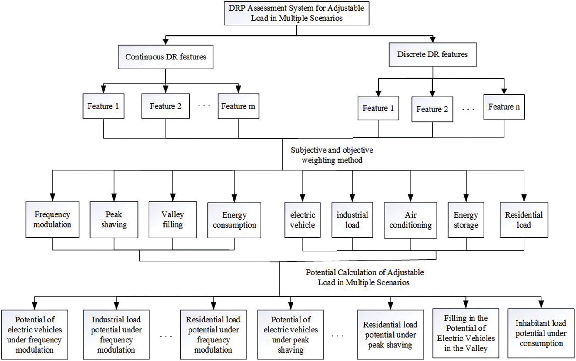
Figure 5: Potential assessment system for adjustable Load DR in DR scenarios

5  Example Analysis

To verify the effectiveness of the proposed model, the article analyzes the results of similar day clustering, time series decomposition, redundancy processing, and model prediction. And verify load DPR in frequency modulation, peak shaving/valley filling, and new energy consumption scenarios. The experimental environment used is a 12th Gen Intel (R) Core (TM) i5-12500H 2.50 GHz CPU, operating system win11, an algorithm written in Python.

The article takes the actual case of LA participating in DR in a certain area of Shanxi Province in February 2021 as the research object. LA obtains information on the participation of adjustable loads in DR through smart meters. Under this LA, 158 users represent adjustable loads, including electric vehicles, industrial loads, commercial loads (mainly air conditioning loads), residential loads, and energy storage. The frequency of data collection is 15 min per point. The following Fig. 6 shows the curve of electric vehicles and commercial loads participating in DR on February 5th under LA.

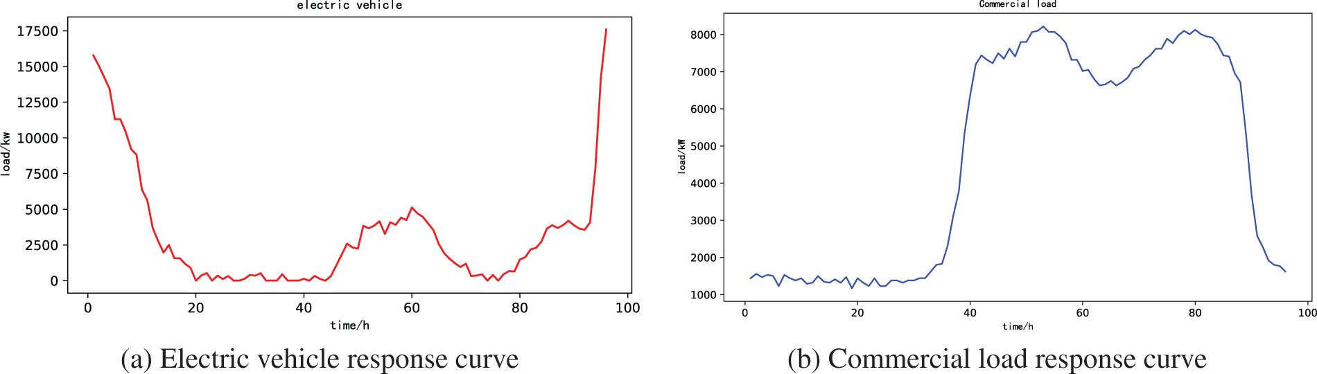
Figure 6: Adjustable load response curve chart

As shown in the figure, electric vehicles mainly participate in DR at night, following the rule of “working during the day and charging at night”; The period for commercial loads to participate in DR is mainly concentrated during the day, which conforms to the rule that “the day is the main electricity consumption period”.

5.1 Analysis of DRP Feature Results Based on Data Mining

5.1.1 Similar Day Clustering Results Based on AP

Cluster the electricity consumption of different loads for February using the AP clustering algorithm. The article takes the electric vehicle as an example and inputs 7 characteristic variables, such as maximum load and peak valley difference rate. The results are shown in Fig. 7 and Table 3 below.

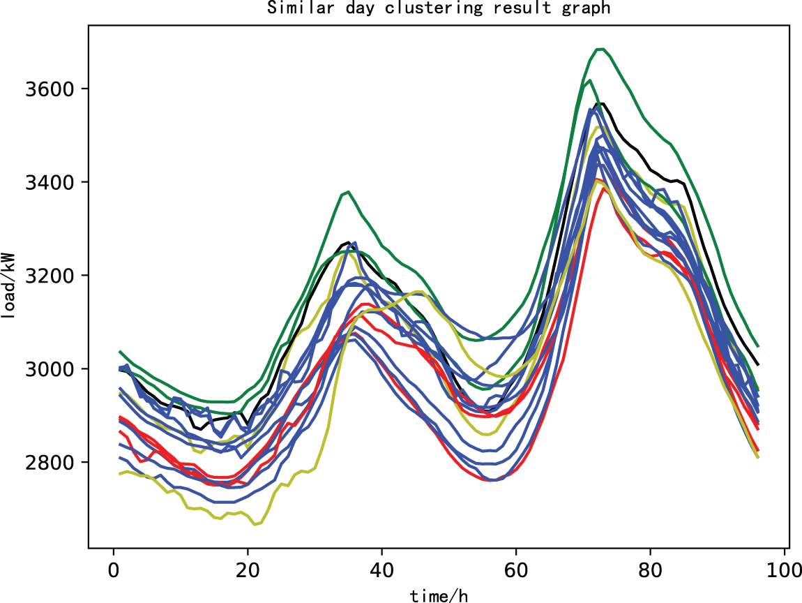
Figure 7: Similar day clustering curve based on AP algorithm

From Fig. 7, it can be seen that the daily electricity consumption pattern of the load is relatively fixed with peak electricity consumption periods at 12:00 noon and 20:00 evening; 5:00 am and 2:00 pm are the periods of low electricity consumption.

According to Table 3, the similarity day clustering based on the AP algorithm divides the data into 6 categories; similar days tend to have similar electricity consumption patterns between adjacent dates, such as February 3rd, February 4th, and February 5th in Cluster 2, which have similar daily load curves; the periodicity of similar days tends to be stronger, which confirms that the electricity consumption patterns of working days and rest days are not the same. For example, in Cluster 3, February 6th, February 7th, February 13th, and February 14th are rest days, while in Cluster 4, February 9th, February 10th, February 17th, and February 18th are working days.

To verify the superiority of the AP clustering algorithm, the AP algorithm is compared with the K-means algorithm, and the clustering results of the above algorithms are evaluated using the average contour coefficient. The average contour coefficient is the average of all sample contour coefficients, as follows:

S=1n∑i=1nbi−aimax{ai,bi}(15)

where ai denotes the average distance between the data of the item i and other samples in this cluster, used to characterize the clustering degree of this cluster; bi denotes the average distance between the data of the item i and samples in other clusters, used to characterize the degree of separation from other clusters. The closer the value is to 1, the better the clustering effect; the closer it is to −1, the worse the clustering effect.

The average contour coefficients obtained through two clustering methods are 0.6123 (AP) and 0.5034 (K-means), respectively. The results indicate that the AP algorithm performs better in clustering.

Based on Fig. 8 and Table 3, it can be concluded that Cluster 3 and Cluster 5 mainly consist of rest days with smaller fluctuations compared to working days. The article selects Cluster 2 data with the highest volatility for analysis with the 26th as DR day and the remaining data as historical data before DR day.

Figure 8: Actual load and response load decomposition curve

5.1.2 Load Time Series Decomposition Results Based on EEMD

Based on the data from similar days in Cluster 2 selected above, the article analyzes the 96-point response load and actual load of electric vehicles on February 3rd. Fig. 8 shows the decomposition curve of the actual load and response load based on the EEMD algorithm. The horizontal axis represents a time series of 96 points a day and the vertical axis represents the electricity consumption and response of load. The electricity consumption and response are both decomposed into five components: IMF1-IMF4 and REST.

According to the characteristics of the EEMD algorithm decomposition curve and the characteristics of actual load and response load, the actual meaning represented by each component is as follows:

For the actual electricity load curve, the fluctuation frequency of IMF1 is relatively high, reflecting the main electricity consumption behavior of adjustable load; The change in IMF2 exhibits symmetry, reflecting the regularity of users’ electricity consumption behavior; IMF3 and IMF4 exhibit significant volatility, reflecting electricity consumption behavior over a longer time scale and unique electricity consumption behaviors, such as peak electricity consumption periods; The last component is the residual component, which represents the trend of electricity consumption. Fig. 8a indicates that the daily electricity consumption of this load is gradually increasing.

For the response load curve, the fluctuation frequency and discrete type of IMF1 are relatively large, reflecting the main response behavior of adjustable load; IMF2 and IMF3 have significant volatility, reflecting electricity consumption behavior in a short period and their unique electricity consumption behavior; IMF4 reflects the electricity consumption behavior of users over a longer time scale; The last component is the remaining component, which generally represents the electricity consumption trend. Fig. 8b above shows an upward trend.

5.1.3 Analysis of Redundancy Processing Results

Based on the features obtained above, the redundancy relationship between features is explained through PCC. The specific results are shown in Fig. 9.

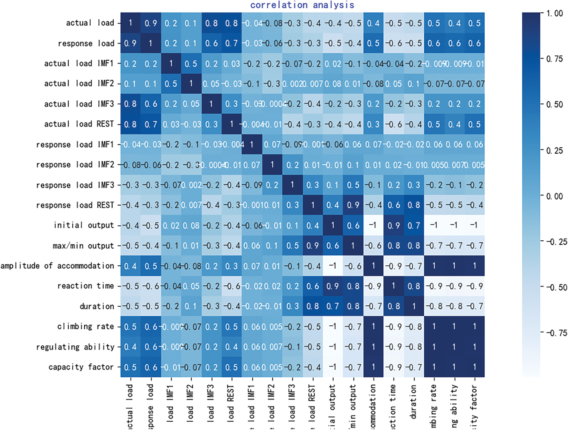
Figure 9: Redundancy analysis result chart

Fig. 9 shows the analysis of redundancy between various features in the obtained historical features. From the graph, it can be seen that there is a strong correlation between initial output, maximum/minimum output and adjustment amplitude, initial output and baseline load, maximum/minimum output and actual load, baseline load, actual load, and response load. Because the adjustment amplitude is the difference between the initial output and the maximum/minimum output; The initial output and baseline load both indicate that the user has not participated in DR; The maximum/minimum output and actual load both represent the user’s participation in DR; The response load is the difference between the baseline load and the actual load. So, keep the response load and remove other features. As a result, the number of features in the feature set is reduced, and the computational efficiency of the model is improved. Finally, after redundancy processing, the extracted DR features are DR quantity, DR reaction time, DR duration, regulating ability, and DR capacity ratio.

5.1.4 GPR-Based Feature Data Extraction and Prediction Results

Use the prediction model constructed above to predict the extracted DR feature set. The prediction results based on GPR are shown in Fig. 10.

Figure 10: Load response power curve with data mining

The algorithm used in general prediction models is a neural network algorithm. To verify the superiority of continuous data volume prediction models based on GPR compared to neural network prediction models, MAE and RMSE are used as indicators to compare the prediction results of GPR with BP and LSTM.

From Table 4, it can be seen that the error based on the GPR algorithm is the smallest; The error of the BP algorithm is the largest; The error of the LSTM algorithm meets the requirements, but it is only a numerical prediction, not a probability distribution. In summary, the GPR algorithm is the best algorithm for predicting continuous indicator data in articles.

To highlight the advantages of data mining, the article also directly inputs data that has not undergone data decomposition, redundancy processing, and other processes into the GPR model. The specific results are shown in Fig. 11.

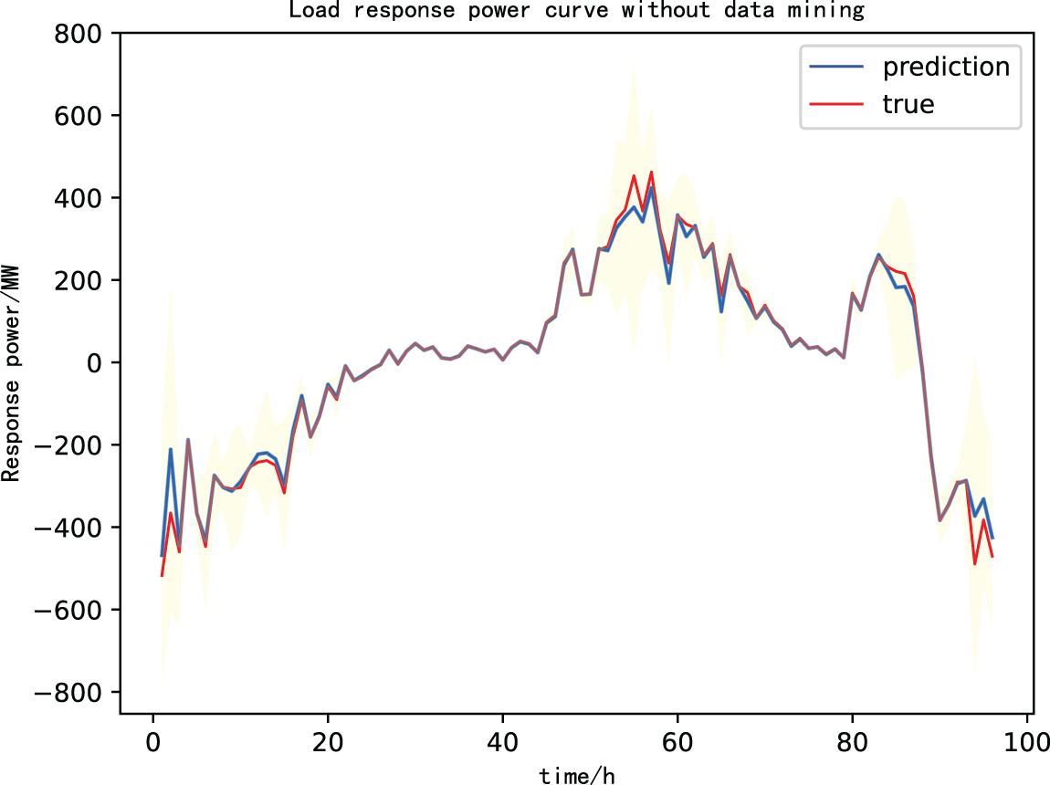
Figure 11: Load response power curve without data mining

From the comparison chart, it can be analyzed that the correlation between the dataset and the predicted values after data mining is higher, and the prediction accuracy is higher, especially for data with large response volumes, which can highlight the advantages of data mining. In addition, according to Fig. 11, it can be analyzed that the load has a strong ability to adjust at night, which means it can consume more electricity than normal electricity usage. It is suitable for consuming new energy at night and filling the electricity trough at night; The ability to reduce electricity usage is relatively strong around 3 pm, which is suitable for reducing electricity load during peak electricity usage in the afternoon.

5.1.5 Analysis of Feature Data Extraction and Prediction Results Based on Data Mining

Table 5 lists the predictive data of various evaluation indicators that characterize the DR process and DR behavior for 5 representative loads out of 158 adjustable load resources from 22:00 to 22:15.

As shown in the table, at this moment, the various indicators of different adjustable loads are different. In terms of response capacity, the industrial load has a significant advantage at 25.4 kw, which is in line with the high capacity characteristics of industrial load; The response between residential load and commercial load is small, only 1 kw, because the residential load and commercial load during this period are in a low electricity consumption period and are not suitable for participating in DR. In terms of reaction time, the energy storage time is the shortest, in the order of seconds, because energy storage is the last resort for DR regulation and operates completely following the DR signal. In terms of duration, industrial load and commercial load perform better, at the minute level. Because both types of loads are regulated uniformly. In terms of regulation ability, electric vehicles are the most flexible because as a new type of load, they can serve as both a means of peak shaving and valley filling regulation.

5.2 Establishment and Advantage Analysis of Evaluation System in DR Scenarios

The article selects four specific scenarios for analysis: frequency modulation, peak shaving, valley filling, and new energy consumption. For frequency modulation, there is usually a peak of electricity consumption, usually from 18:00 to 20:00 and the article is set to 19:00; for peak shaving scenarios, it is generally 8:30 to 10:30, 18:00 to 19:00, 20:00 to 23:00 and the article is set to 18:00, with a large DR volume; for grain filling scenarios, it is generally 0:00–8:00 and the article is set to 0:00, resulting in a large amount of DR; for new energy consumption, the typical scenario for this new energy consumption is set to have surplus wind power generation at night, and the article is set at 2:00 am.

5.2.1 Analysis of DR Potential for Adjustable Load in DR Scenarios

Through the modeling and analysis of the DR scenarios mentioned above. The specific parameters for the four scenarios of frequency modulation, peak shaving, valley filling, and new energy consumption established in the article are shown in Table 6.

The adjustable parameters of various indicators of adjustable load are shown in the predicted results in Table 6 above. Then, objective weights and combination weights of each DR scenario and adjustable load are obtained through the AHP and CRITIC weighted subjective and objective weight analysis, as shown in Tables 7 and 8.

According to Table 7, by calculating the subjective and objective weights for the characterization of DR processes and behaviors under different adjustable loads, it can be concluded that in terms of response quantity, large-scale industrial loads have the largest response quantity, for nearly 0.5; In terms of reaction time, energy storage enterprises have the fastest reaction time, for 0.38; In terms of response duration, the proportion of industrial load and air conditioning can both reach 0.3 due to the longer operating load time; In terms of regulation ability, electric vehicles, and energy storage enterprises have relatively flexible conditions, which can be manifested as both upward regulation response potential and downward regulation response potential; In terms of capacity ratio, energy storage, and electric vehicles exhibit a larger capacity ratio, making them more suitable as adjustable loads to participate in demand response. From both subjective and objective weights, it can be seen that large industrial loads, electric vehicle companies, and air conditioning have a stronger willingness to respond. Because industrial loads have the characteristics of large load capacity and unified regulation, DR has a strong DPR in terms of focusing on response quantity and duration; Electric vehicles are more suitable for DR scenarios due to their flexible adjustment; Energy storage, as an adjustable load generated by DR, has various indicators, but due to its high cost, it is generally not the preferred load for LA regulation.

While evaluating the DRP for different loads, the article also calculated the weight of evaluation indicators for DR potential requirements for four DR scenarios: frequency modulation, peak shaving, valley filling, and new energy consumption. The details are shown in Table 8.

According to Table 8, by calculating the subjective and objective weights of the characterization DR process and behavior of different adjustable loads, it can be concluded that the frequency-modulated DR requires the highest response time for load participation in DR, which is 0.450. This confirms the conclusion that the frequency-modulated DR scenario requires a fast response time for adjustable loads; The peak shaving and valley filling DR have high requirements for load regulation ability and response quantity, with values of 0.259 and 0.286, respectively. Because peak shaving and valley filling require adjustable loads to consume less electricity during peak periods and more electricity during low periods; The new energy consumption type DR has the highest response requirement for adjustable loads, which is 0.605. This scenario solves the problem of excessive new energy generation, which leads to an imbalance between electricity supply and demand.

For the DRP of different loads and response requirements for different DR scenarios, Table 9 provides a detailed analysis and comparison of the DR potential of different loads under different response scenarios.

According to Table 9, different types of adjustable loads need to be mobilized for different DR scenarios. In terms of overall comprehensive DR potential, large industrial enterprises, electric vehicles, and energy storage have better response effects, with DRP above 0.2 for each load. In contrast, the DPR of residential load is relatively low, all around 0.1, due to the dispersed distribution of residential load, small capacity, and strong randomness; For frequency-modulated DR, the DRP performance of energy storage is outstanding, at 0.444. Due to the fast response of energy storage, it is most suitable for frequency modulation DR scenarios; For peak shaving and valley filling DR, electric vehicles, industrial loads, and energy storage all have good DRP. Due to the DPR of electric vehicles having both upward and downward adjustment capabilities, electric vehicles have better DRP compared to industrial loads and energy storage; For new energy consumption type DR, industrial load has outstanding advantages at 0.559. The second highest is electric vehicles, at 0.448. Because of the large capacity of industrial loads. Although electric vehicles have a small individual capacity, they have a large volume.

5.2.2 Analysis of the Advantages of Potential Evaluation System

To highlight the advantages of the established DRP evaluation system, the article analyzes the following three situations:

Case 1: Only the response power of adjustable loads is used as a DRP evaluation indicator;

Case 2: Establish a DRP assessment system that only analyzes the DRP of adjustable loads;

Case 3: The system established in this article analyzes the DRP of adjustable loads in different DR scenarios.

For simplicity, the load of electric vehicles is represented by ‘1’; the industrial load is represented by ‘2’; the air conditioning load is represented by ‘3’; energy storage is represented by ‘4’; the residential load is represented by ‘5’. Scenario 1 is obtained by comparing the combined weights of each load response quantity in Table 6, reflecting the basis for the most traditional LA call load to participate in DR response; Scenario 2 is obtained by comparing the weights of each indicator for each type of load in Table 6, reflecting the basis for the most systematic LA call load to participate in DR; Scenario 3 is obtained by comparing the DR potential values of different loads in different DR scenarios according to Table 8, which serves as the basis for the LA call load to participate in DR based on the model proposed in the article. The specific comparison results are shown in Table 10 below:

The sorting of various loads in each case in the table: from left to right, the DR effect is getting worse and worse. Analysis of Table 10 shows that when only considering the demand response of the load, the DR effect of industrial load is the best (case 1); When not considering the DR scenario, the DR effect of energy storage is the best (case 2); When considering both the indicators of load DR and different DR scenarios, the best DR effect is achieved for different loads, such as frequency modulated DR scenarios, where the DR effect of energy storage is the best; The peak shaving DR scenario has the best DR effect for energy storage; In the valley filling DR scenario, electric vehicles have the best DR effect, while new energy consumption scenarios and industrial loads have the best DR effect. Overall, electric vehicles are suitable for a wider range of DR scenarios and have better response effects.

6  Conclusion

At present, mobilizing demand-side resources has become a necessary means. Based on this, the article proposes a DRP prediction model based on data mining and a DRP evaluation model based on subjective and objective weights: by analyzing the DR process and DR behavior, extracting relevant features and comprehensively characterizing the DRP of adjustable loads and DR scenarios, the one-sided representation of DRP solely based on DR power is solved. Then, through the established data mining model, the internal relationships of features are extracted and redundant information and noise information are removed, greatly reducing the dimensionality and data volume of features and solving the problem of low efficiency and accuracy in data calculation and prediction caused by insufficient data volume due to data security; Afterward, a DRP calculation model based on subjective and objective weight calculation is established to calculate DRP comprehensive and reasonable, providing a reasonable basis for load aggregators to adjust load scheduling for different DR scenarios. Finally, simulation verification shows that the prediction model established in the article greatly improves the efficiency and accuracy of data prediction; The DRP based on subjective and objective weight calculation in the DR scenario established by analyzing the DR process and DR behavior is more accurate, comprehensive, and reasonable.

In summary, the data prediction model established in the article improves the efficiency and accuracy of data prediction, making LA timely and accurate in DRP calculation, and laying the foundation for it; By establishing a DRP calculation model, LA calculates adjustable load DRP for different DR scenarios and provides a reasonable basis for formulating reasonable DR plans. The above model maximizes the benefits for LA in participating in DR, improves the effectiveness of DR, and facilitates smoother operation of the DR market.

However, considering the future development of DR, the following suggestions are proposed for the DR evaluation system proposed in the article: combine multi-energy virtual power plants and study the impact of uncertainty in new energy generation on the DRP assessment system; establish a DRP assessment system based on comprehensive DR market in China and different DR projects.

Acknowledgement: Thank you to my teacher, Professor Du Xinhui, for your careful guidance. I also want to thank everyone in the laboratory for their help.

Funding Statement: Project supported by the National Natural Science Foundation of China Youth Fund, Research on Security Low Carbon Collaborative Situation Awareness of Comprehensive Energy System from the Perspective of Dynamic Security Domain (52307130).

Author Contributions: The authors confirm their contribution to the paper as follows: study conception and design: Zhang Zhishuo; data collection: Zhang Zhishuo; analysis and interpretation of results: Zhang Zhishuo; draft manuscript preparation: Zhang Zhishuo. All authors reviewed the results and approved the final version of the manuscript.

Availability of Data and Materials: The data are not publicly available due to their containing information that could compromise the privacy of research participants.

Conflicts of Interest: The authors declare that they have no conflicts of interest to report regarding the present study.

References

1. Xi, J. P. (2020). Speech at the general debate of the 75th session of the United Nations general assembly. Communique of the State Council of the People's Republic of China, 2020(28), 5–7 (In Chinese). [Google Scholar]

2. Wang, F., Li, M. Y., Zhang, X. D. (2023). Methods, applications, and prospects of demand response resource potential assessment. Power System Automation, 47(21), 173–191. [Google Scholar]

3. Wang, C. X., Shi, Z. Y., Liang, Z. F. (2021). Key technologies and prospects of demand-side resource utilization for power systems dominated by renewable energy. Automation of Electric Power Systems, 45(16), 37–48. [Google Scholar]

4. Yang, J. X., Li, Q. H., Zhang, Y. J. (2021). Peak shaving optimization modeling for demand response of multiple EV aggregators considering matching degree of power grid demand. Electric Power Automation Equipment, 41(8), 125–134. [Google Scholar]

5. Wang, M. L., B.B., S., Wang, L. Y. (2023). Research on energy green and low carbon transformation from the perspective of policy tools. Green Technology, 25(9), 240–246. [Google Scholar]

6. Zeng, M., Zhang, S. (2023). Analysis of China’s energy system construction during the 14th five year plan. China Electric Power Enterprise Management, 2023(25), 65–67. [Google Scholar]

7. Wan, Q. L. (2015). Potential and obstacles of residents’ user demand response in Sweden. Power Demand Side Management, 17(6), 62–64. [Google Scholar]

8. Torstensson, D., Wallin, F. (2015). Potential and barriers for demand response at household customers. The 7th International Conference on Applied Energy (ICAE), Amsterdam, Elsevier. [Google Scholar]

9. Ziras, C., Heinrich, C., Pertl, M. (2019). Experimental flexibility identification of aggregated residential thermal loads using behind-the-meter data. Applied Energy, 242, 1407–1421. https://doi.org/10.1016/j.apenergy.2019.03.156. [Google Scholar] [CrossRef]

10. Wu, Z. D. (2020). Research on key technologies of demand response (Master Thesis). South China University of Technology, China. [Google Scholar]

11. Sheidaei, F., Ahmarinejad, A. (2020). Multi-stage stochastic framework for energy management of virtual power plants considering electric vehicles and demand response programs. International Journal of Electrical Power & Energy Systems, 120, 106047. https://doi.org/10.1016/j.ijepes.2020.106047. [Google Scholar] [CrossRef]

12. Kong, X. Y., Liu, C., Wang, C. S. (2022). Demand response potential assessment method based on deep subdomain adaptation network. Proceedings of the CSEE, 42(16), 5786–5797 (In Chinese). [Google Scholar]

13. Luo, J. M., Wen, Z. C., Dong, W. J. (2020). Model of integrated demand response potential based on a portrait of residential users. Renewable Energy Resources, 38(10), 1407–1414. [Google Scholar]

14. Wu, D., Wang, Y. C., Yu, C. L. (2022). Demand response potential evaluation method of industrial users based on Gaussian process regression. Electric Power Automation Equipment, 42(7), 94–101. [Google Scholar]

15. Zong, J. F., Wang, C., Shen, J., Su, C. H., Wang, W. Z. (2023). ReLAC: Revocable and lightweight access control with blockchain for smart consumer electronics. IEEE Transactions on Consumer Electronics. [Google Scholar]

16. Xu, D. Q., Peng, C. G., Wang, W. Z., Liu, H., Shaikh, S. A. et al. (2023). Privacy-preserving dynamic multi-keyword ranked search scheme in multi-user settings. IEEE Transactions on Consumer Electronics, 69(4), 890–901. https://doi.org/10.1109/TCE.2023.3269045. [Google Scholar] [CrossRef]

17. Wang, W. Z., Han, Z. Y., Raza, S., Tanveer, J., Su, C. H. (2023). Lightweight blockchain-enhanced mutual authentication protocol for UAVs. IEEE Internet of Things Journal. [Google Scholar]

18. Wang, F. Y., Liu, M., Li, Q. S. (2023). Evaluation of demand response potential of power users in new power systems. Electrical Measurement and Instrumentation, 60(8), 105–113+132. [Google Scholar]

19. Hand, D. J. (2007). Principles of data mining. Drug Safety, 30, 621–622. https://doi.org/10.2165/00002018-200730070-00010 [Google Scholar] [PubMed] [CrossRef]

20. Tan, P. N., Steinbach, M., Kumar, V. (2013). Introduction to data mining, Pearson new international edition. Pearson Schweiz Ag, 14(2), 279–288. [Google Scholar]

21. Li, H. L., Zhang, L. P. (2022). Summary of clustering research in time series data mining. Journal of University of Electronic Science and Technology, 51(3), 416–424. [Google Scholar]

22. Mu, Y. K., Wang, L. T. (2022). Line fault location based on complementary set empirical mode decomposition. Electrical Automation, 44(05), 63–65. [Google Scholar]

23. Qi, X. J., Ji, Z. S., Wu, H. B. (2020). Short-term reliability assessment of generating systems considering demand response reliability. IEEE Access, 8, 74371–74384. https://doi.org/10.1109/Access.6287639. [Google Scholar] [CrossRef]

24. Li, M. Y., Li, G. J., Wang, K. Y. (2023). A bidding strategy for virtual power plants considering demand response and frequency modulation performance changes. Power System Protection and Control, 51(3), 13–25. [Google Scholar]

25. Yang, J. X., Li, Q. H., Zhang, Y. J. (2021). Modeling of peak shaving optimization for multi EV aggregator demand response considering grid demand matching. Power Automation Equipment, 41(8), 125–134. [Google Scholar]

26. Zhang, Y. X., Liu, W. Y., Pang, Q. L. (2023). Multi-time scale optimization scheduling strategy considering comprehensive demand response participation in the absorption of hindered new energy. Electric Power Construction, 44(1), 1–11. [Google Scholar]

27. Liu, D. Q., Zhang, X., Qian, Y. H. (2023). Game collaborative strategy for the evolution of electric vehicle cluster charging and discharging. Power System Protection and Control, 51(16), 84–93. [Google Scholar]

28. Fan, D. J., Zhang, S., Wang, Y. (2022). The day ahead dispatching strategy of air conditioning load aggregator considering the diversity of user regulation behavior. Power System Protection and Control, 50(17), 133–142. [Google Scholar]

29. Chen, G. Y., Yang, X. Y., Jiang, H. Y. (2023). Power grid demand response regulation strategy considering industrial load characteristics under a high proportion of new energy access. Power Automation Equipment, 43(4), 177–184. [Google Scholar]

30. Deng, R. Y., Cheng, X. K., Zou, P. L. (2023). Research on the evaluation system of humanities airport based on fuzzy analytic hierarchy process. Computer Age, 2023(8), 121–124+128. [Google Scholar]

31. Chen, C., Yan, X. Y., Qi, H. R. (2023). Evaluation method for rooftop photovoltaic access distribution network based on FAHP improved CRITIC combination weighting. Power System Protection and Control, 51(15), 97–108. [Google Scholar]