Transient Stability Preventive Control of Wind Farm Connected Power System Considering the Uncertainty

Nomenclature

1  Introduction

The essential methodology of system transient stability preventive control (TSPC) is to reschedule the power generation subject to transient stability constraint [1] in order to avoid power systems from the risk of falling out of step after potential contingencies. It provides the guarantee for the safe and stable operation of the power grid and has always been an attractive theme to system operators. Transient stability preventive control is considered as an implementation of transient stability constrained optimal power flow (TSCOPF) as well [1] since it provides a system operation strategy with security boundaries.

Compared with traditional static optimal power flow (OPF), the pivotal part of TSCOPF involves handling the transient stability constraints (TSC) derived from the complex differential algebraic equations (DAEs) of power systems. The presently available approaches to this issue can generally be classified into the discretization-based method and the decomposing iteration method. The former approximates the differential equations into equivalent algebraic forms based on the numerical discretization technique and the stability constraints are directly embedded into the OPF process. So the dynamic limitations are transformed as a set of inequality constraints and then the semi-infinite TSCOPF programming into a large-scale finite-size optimization. This introduces the increase of variables, constraints, and then the computation time inevitably. In reference [2], the authors reduce the transient stability dimension based on the Single Machine Equivalent method which simplifies the multi-machine system to an equivalent one-machine infinite-bus system. However, it may lead to inaccurate modeling of the system’s dynamic behavior when dealing with large-scale power systems and wind turbine modeling. Reference [3] introduces a parallel reduced-space interior point method (IPM) to relieve the computing burden for multi-contingency TSCOPF problems. Although considerable efforts have been made, the discretization-based method might still be computationally intractable, particularly in real power systems. The latter method decomposes the TSCOPF into an OPF subproblem and a transient stability analysis (TSA) subproblem, afterward the two subproblems are solved alternately, and the optimal operation point is achieved iteratively, so the policy is defined as a “sequential” approach [4]. A divide-and-conquer approach is presented in reference [5] to solve TSCOPF by decomposing it into OPF and TSC subproblems and these two subproblems are solved by IPM and energy sensitivity technique.

The researches aforementioned have not covered wind farm power systems which have been rapidly growing for the sustainable development demand in the last decade. The integration of wind turbines has brought a significant challenge to the TSCOPF research, especially the introduced uncertainty of variables. The difficulty mainly lies in dealing with uncertainty and transient stability problems simultaneously. Reference [6] adopts a chance-constrained optimization model for the randomness of wind power. As for the system transient constraint, a transient stability correction strategy based on trajectory sensitivity is proposed. The transfer active power for reducing the rotor angle difference is calculated based on the trajectory sensitivity method and then is shifted from the most advanced generator to the least advanced one directly. So the generation re-dispatch scheme may not necessarily be the most optimal one. Reference [7] proposes a probabilistic contingency severity index based on random factors and embeds it into dynamic reactive power planning. In reference [8], the transient stability constraint is expressed in its probabilistic form and the problem is modeled as a probabilistic TSCOPF problem. However the transient stability analysis in these references is based on time domain simulation, so it is very time-consuming. Generally speaking, the existing research is not rich enough and deserves more investigation in this area.

In addition, the multi-objective optimization model is often used in power system optimization for its concern with multiple objective functions. Reference [9] presents a multi-objective optimization model for the dynamic feeder reconfiguration problem which considers operational cost, energy loss, and voltage stability index as objective functions that can meet operational and voltage security expectations. For energy management in the distribution network, reference [10] considers energy loss, voltage stability index, and operational cost as objective functions in the presence of distributed generators, solar PV panels, ES units, and capacitors.

Inspired by the alternate optimization idea of the sequential approach, a novel three-stage probabilistic multi-objective TSCOPF (PMO-TSCOPF) framework addressed to TSPC of wind farm power systems is proposed in this paper. The optimal solution will be achieved by the satisfaction of the static chance constraints and the dynamic steady constraints alternately in the three stages. Chance-constrained optimizing model based on the point estimate method (PEM) is adopted for the uncertain factors of the wind farm system. Multi-contingencies can be considered during the transient stability feasible domain confirming procedure. The main contributions of this work are as follows:

• Addressed to TSPC in wind farm power system, we extend chance-constrained OPF to the TSPC problem and formulate a PMO-TSCOPF model which incorporates uncertainty, TSC, and multi-objective optimization issues into a whole optimization procedure, and then obtain the optimal operating scheme successfully.

• A three-stage PMO-TSCOPF framework that combines the probabilistic multi-objective PSO (P-MOPSO) method and the deterministic IPM is presented. It is general to support other optimal algorithms for handling probabilistic programming problems combined with security constraints. And it is still flexible to accommodate more detailed modeling. This provides a new train of thought for solving the optimization problem which considers uncertainty and transient stability at the same time.

• The approach proposed in this study introduces a modified objective function form for multi-objective chance-constrained optimization. As a result, low-carbon emission, as well as the operation cost, is embedded in the multi-objectives optimization for environmental consideration. In addition, multi-contingencies can be considered during the transient stability feasible domain confirming procedure.

The rest of the paper is organized as follows. The problem and the mathematical formulation are presented in Section 2. Section 3 describes the proposed approach of PMO-TSCOPF in detail. Section 4 is the numerical result and analysis, and the conclusion is in Section 5.

2  Problems and Mathematical Model

2.1 Preventive Control Formulation of Power System with Wind Generation

To ensure the optimal objective in the sense of average level, the objectives employ the expectation forms. To avoid the increased expense caused by the demand for rigid constraints, the chance constraints are adopted. Thus, the general probabilistic preventive control formulation can be represented as:

MinE{f}(1)

S.T.h(u,x,ξ)=0(2)

Pr{g(u,x,ξ)<0}>β(3)

where u,x, and ξ are the control variables, state variables, and random input variables in turn. E{f} means the mathematical expectation of the function f; and Pr{⋅} stands for the probability of the event {⋅}. β is the confidence degree of chance constraints which means the probability of constraint being satisfied will be guaranteed greater than β level. So E{f} is the objective function to be minimized, h and g are the equality and inequality constraints.

2.1.1 Objective Functions

Different from traditional single objective OPF, the objective functions of the formulation in this paper are comprised of two subordinate objectives:

f={f1,f2}(4)

f1=∑i=1NG(aiPGi2+biPGi+ci)(5)

f2=∑i=1NGλiPGi(6)

where ai, bi, ci are the fuel cost coefficients and λi is the carbon emission intensity of the i−th conventional thermal power generator. PGi is the output active power of this generator and NG is the total number of thermal power generators in the grid.

The objective functions indicate the two concerning issues, respectively: the sub-objective f1 accounts for the generation cost and f2 is the amount of pollution gas emission of the power grid.

Compared with many earlier works whose focuses are single objective chance-constrained optimization or its transformation from references [11,12], the approach proposed here contributes a new way to multi-objective chance-constrained optimization. So the objectives can still include more subjects such as network loss [13], NOX emission [14], etc.

2.1.2 Constraints

The steady-state constraints in optimization model Eqs. (1)–(3) are power flow equations and static operation restrictions:

{Pi−Vi∑j∈iVj(Gijcosθij+Bijsinθij)=0Qi−Vi∑j∈iVj(Gijsinθij−Bijcosθij)=0(7)

PGimin≤PGi≤PGimaxQGimin≤QGi≤QGimax(i=1,2…NG)(8)

Pr{Vimin≤Vi≤Vimax}≥βV(i=1,2…NB)(9)

Pr{|Si|≤Simax}≥βS(i=1,2…NL)(10)

in which, Pi and Qi are the injected active and reactive power of node i, Vi is the bus voltage magnitude, Gij and Bij are the conductance and susceptance of the branch between node i and j, θij is the angle between the two nodes. PGimin, PGimax and QGimin, QGimax are the output limits of generator i; Vimin, Vimax, and Simax are bus voltage and branch power limits, respectively; βV and βS are the confidence levels of node voltage and branch power constraints. NB and NL are the numbers of nodes and branches in the grid.

2.1.3 Transient Stability Constraint

The transient stability requirement of the system operation is restricted by TSC. Like most references [15,16], the TSC here employs the maximum allowable generator rotor angle deviation with respect to the center of inertia (COI) after contingencies as the transient stability assessment criterion. The formulation can be indicated as:

Max {|δi−δCOI|}≤ρ(11)

δCOI≜1∑i=1NGMi∑i=1NGMiδi(12)

where δi and Mi are the rotor angle and inertial moment of i−th generator, δCOI is defined as the angle of the inertia center and ρ is the threshold of the rotor angle deviation in COI system which is ρ normally set to π.

The utilization of COI coordinate eliminates the rotor angle deviation error caused by the movement of the inertia center, which does not reflect the out-of-step of the power system.

2.2 Mathematical Model

2.2.1 The Uncertain Model of Wind-Farm-Connected Power System

The output power of wind farm is directly influenced by the wind speed which follows the Weibull distribution statistically and the probabilistic density function (PDF) of the average wind speed can be expressed as:

f(v)=kc(vc)k−1exp⁡[−(vc)k](13)

where v is the wind speed (m/s); k and c are the shape and scale parameters, respectively. The output power of wind turbine can be calculated from wind speed information according to:

Pw={0v≤vciorv>vcoPN(v−vcivN−vci)vci<v≤vNPNvN<v≤vco(14)

in which vci, vco, and vN are the cut-in, cut-out, and nominal wind speed, and PN is the rated active power of wind turbine.

Another uncertainty source in wind farm system is power load which behaves as normal distribution approximately, and the PDF is:

f(p)=1σ2πe−(p−p¯)22σ2(15)

where p is the load power, p¯ and σ are the mean and standard deviation of it.

2.2.2 The Dynamic Model of System

The probabilistic models of wind farm and load are employed in the stochastic power flow calculation for the static optimization program, but in the time domain simulation (TDS), the dynamic model should be specified.

The synchronous generator is modeled as the fourth-order dynamic generator model with the state variables rotor angle, rotor speed, the q-axis, and d-axis transient voltages.

The doubly-fed induction generators (DFIGs) are extensively applied in the wind farm for their excellent control characteristic. The wind farm is aggregated as a single equivalent DFIG turbine model in this work for simplicity. Although DFIGs do not suffer from angle instability problems themselves because of their asynchronous operation, they still have a considerable influence on the transient stability process for their rapid change of output power after the contingency. To realize the decoupled control of active & reactive power, the DFIGs are attached to the grid through the 3-phase back-to-back PWM converters as depicted in Fig. 1.

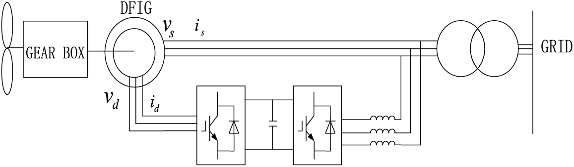
Figure 1: The structure of DFIG based system

By disregarding the dynamics of the stator and rotor flux, the simplified DFIG dynamic model representation is:

{vds=−rsids+((xs+xm)iqs+xmiqr)vqs=−rsiqs−((xs+xm)ids+xmidr)(16)

{vdr=−rridr+(1−ωw)((xr+xm)iqr+xmiqs)vqr=−rriqr−(1−ωw)((xr+xm)idr+xmids)(17)

Pw=vdsids+vqsiqs−vdridr−vqriqrQw=vqsids−vdsiqs(18)

3  Proposed Methodology

To solve the PMO-TSCOPF problem, a three-stage strategy that integrates the chance-constrained multi-objective PSO (MOPSO) method and IPM is implemented in this paper. At first, a rough ideal operation domain is figured out by the probabilistic PSO (P-PSO) method ignoring the transient constraints, and then it shrinks to the transient stability feasible region for contingencies consideration by IPM. Finally, the optimal operating point that satisfies both the transient limitation and the chance constraints is settled in the third stage. The main technical features are as follows: probability power flow calculation, the modified MOPSO method, and the TSC-feasible region confirming for contingency and even expanded for multi-contingencies.

3.1 PEM for Power Flow

The probability of constraints satisfaction is accomplished through the calculation of stochastic power flow. The most common algorithms for stochastic power flow are the Monte Carlo Simulation (MCS) method [18], the cumulant method [19], and PEM, etc. The MCS method is mathematically accurate but has the shortcoming of heavy computation. Analytical methods such as cumulant-based power flow require more assumptions and complicated computation which constrain their further application.

PEM [20,21] is a numerical method that gives the moments of output random variables only by several deterministic power flow computations, and then the approximate probability density distribution can be figured out through Gram-Charlier expansion [22]. With its high analytical accuracy and acceptable computation burden, PEM has been applied in the probabilistic power flow computation of this paper.

3.2 Multi-Objective Chance-Constrained Optimization Based on PSO

The optimization tendencies of the two sub-objective functions in this multi-objective OPF (MO-OPF) model are probably inconsistent with each other. The Pareto solution provides the key to the multi-objective optimization problem that has incompatible objectives. The Pareto optimal set is a set of non-dominated solutions whose sub-objectives are not inferior to others.

PSO method is considered one of the most effective intelligent optimization algorithms especially for multi-objective problems because it can create uniformly distributed Pareto sets [23]. The MOPSO method used in this study is developed from the version in references [24], which utilizes adaptive hyper-cubes for the pruning of the Pareto solutions in the external archive. The particle xi in the swarm is updated according to the local best solution pb and the global best solution pg, and the renewal formulas of particle velocity vi and particle xi are as follows:

vi(t+1)=ωvi(t)+c1rand1(pb(t)−xi(t))+c2rand2(pg(t)−xi(t))(19)

xi(t+1)=xi(t)+vi(t+1)(20)

where t is the iteration order; c1 & c2 are the learning parameters that control the impact of pb & pg; rand1 & rand2 are two uniformly distributed random numbers within 0~1 and ω is the inertia weight factor.

In order to be more suitable to the MO-OPF here, the classical PSO method is modified in some places including the changing inertia weight, the mutation factor, and the quantified penalty function.

The contraction factor χ coupled with inertia weight ω is embedded into the iteration of PSO to improve the performance of the algorithm. For the particle xi, the modified formula for renewal velocity is:

ω=ωmax−ωmax−ωmintmaxt(21)

vi(t+1)=χ∗(ωvi(t)+c1rand1(pb(t)−xi(t))+c2rand2(pg(t)−xi(t)))(22)

χ=2|2−φ−φ2−4φ|,φ=c1+c2,φ>4

in which, ωmax & ωmin are the maximum and minimum values of ω, which are generally set to 0.9 and 0.4. t&tmax are the current iterative order and maximum iterative number. So the inertia weight ω decreases linearly with the iteration as shown in Eq. (21). The earlier higher value enlarges the search range and the later lower value speeds the search process. The implementation of the contraction factor χ has enhanced the convergence of PSO [25] and with the setting of c1=2.05,c2=2.05,φ=4.1, it has the best effect [26].

The mutation factor aims at maintaining the particle diversity and avoiding premature convergence [27]: If the particles stop evolution (i.e., do not show obvious changes) for several (4 to 6) continuous iterations, initialize the particles at a certain probability.

There are several different treatments for optimization constraints utilized in this research. The control variable limitation, i.e., generator output restriction (8) in the preventive control is guaranteed by the initial variables boundary. The infeasible solution represented as violating the equality constraints (7) of power flow is directly eliminated from the PSO particles. For the chance constraints which are not so rigorous exclusive constraints, a quantified penalty function is practiced in the revised objective function:

f′=f×(1+∑i=1Nc′(β−pi)Nc)(23)

In Eq. (23), for the given confidence level β, Nc is the total number of chance constraints, Nc′ is the number of not satisfied constraints and pi is the probability of i−th constraint. So the modified objective function is amplified along with the number and level of violated constraints.

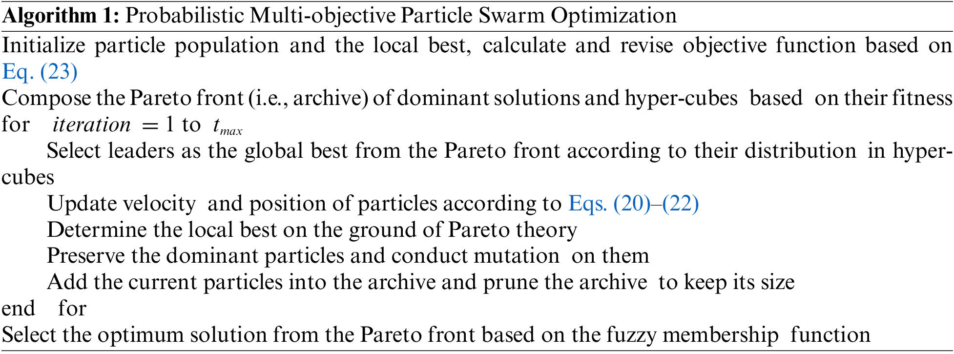
In summary, the pseudo code of the P-MOPSO algorithm can be displayed as:

3.3 The TSC Feasible Region Confirmation for Multi-Contingencies

The transient stability constraints are ensured in the second stage of the whole process. Researches show that transient stability is governed by the active power output of generators [28], so the corresponding constraints can be converted to limitations of machines’ active output in the preventive control. Restricting the active output boundary of generators associated with a certain contingency and shifting part of the generation from the relevant generators to other generators is looked at as the treatment method to transient constraints in TSCOPF [16,20], but the accuracy of the shifted power is still a problem to be solved. Addressed to this question, a deterministic optimization model is added as the second stage of the optimization framework. The objective is the least deviation away from the present operating point, which is the most optimal result acquired from the first stage just without transient constraints:

Min∑i=1NG|ΔPGi|(24)

S.T. PGi−PGimin≤ΔPGi≤PGimax−PGi(i=1,2,…NG)(25)

Max {|δi−δCOI|}<ρ(i=1,2,…NG)(26)

∑i=1NG(PGi+ΔPGi)−PD−PLoss=0(27)

In the model, the control variable ΔPGi is the adjusted active power of i−th generator, and the constraints include control variable constraints (25), transient stability constraint (26), and power balance constraint (27) in turn. The optimization model is solved by the numerical discretization methodology with the demand that the constraints should be guaranteed during the TDS.

The embedded IPM optimizer in MATLAB is selected as the optimization tool and the details of the optimization method can be found in reference [21]. Each minus ΔPGi of the optimal result is the re-constrain of the relevant generator for modifying its maximum output limitation and then the TSC feasible region associated with this contingency is confirmed. This method is suitable for multi-contingencies: Execute one optimization for every single contingency separately and the common part of generation limitation for all contingencies is the system TSC- feasible region.

3.4 The Complete Framework

The whole computation process of the proposed strategy can be summarized in the following steps and the flow chart in Fig. 2:

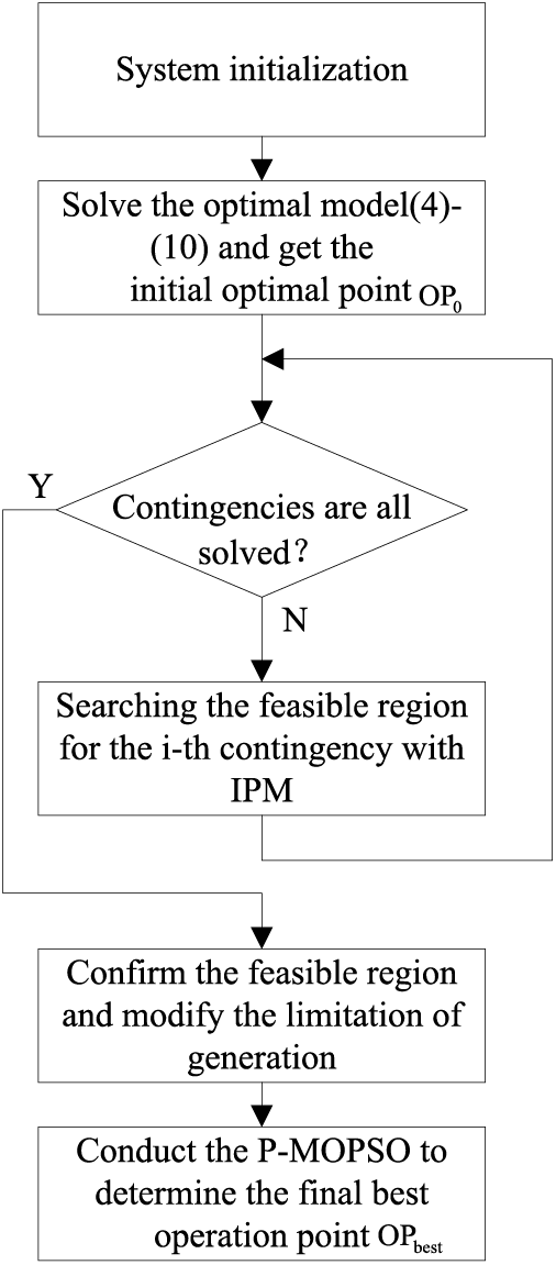
Figure 2: The flow chart of the proposed strategy

Step 1: The system and the generation boundaries of all generators are initialized.

Step 2: Solve the optimal model (4)–(10) with the P-MOPSO method ignoring TSC and get the initial optimal operating schedule OP0.

Step 3: Check the contingencies set and go to step 5 if there are no unsolved contingency constraints; otherwise go to the next step.

Step 4: Conduct the optimization of model (24)–(27) under the i−th contingency without chance constraints on the basis of point OP0 and go back to step 3.

Step 5: Confirm the TS security feasible solution region for all contingencies and modify the limitation of the generator’s active power output.

Step 6: Perform the chance-constrained MOPSO in the found TS security feasible region and get the final best solution OPbest.

4  Case Study

The proposed method is demonstrated on the modified WSCC 9-bus system and the New England 39-bus system to verify its effectiveness. The tests are all carried out on an Intel corei5 processor with 8 GB RAM. The algorithm is programmed in MATLAB2013a with the static OPF developed based on the MATPOWER4.0 package [29], and the TSCOPF is performed by MATLAB IP solver with the assistance of PSAT package [30]. The TDS time is set up to 5 s with the integration step of 0.05 s. The population size, repository size, and the maximum number of iterations are set as 20, 50, and 50, respectively. The confidence degrees of bus voltage and branch power are set at the same level β here, which can also be different if necessary.

4.1 WSCC 9-Bus System Connected with Wind Farm

The single-line diagram and detailed data including the fuel cost parameters of the original WSCC 9-bus system are available in reference [31], and the wind farm is directly connected to bus 5 with different wind generation penetration levels. The cut-in, rated and cut-out speeds of the wind turbine are 3, 16, and 25 m/s respectively with the k and c parameters of the wind speed Weibull model being 3 and 14. The load standard deviation σ is 10% of the mean value of load power. The bus voltage limit is 0.95∼1.05p.u. The carbon emission intensity of every synchronous generator is set to 0.9T/MWH.

With the installed capacity of the wind farm being 30 MW, i.e., the penetration level of 9.5%, the initial optimal operating schedules OP0 acquired in the first stage under different confidence levels β are shown in Table 1.

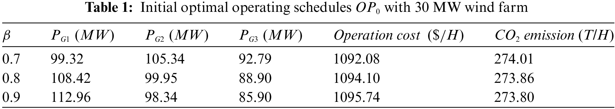
It indicates that with the increase of confidence level, the objective values grow gradually. It is the inevitable cost of the stringent constraints that lead to the narrow feasible solution domain. The amounts of CO2 emission for different operation schemes shown in the last column do not have distinct changes apparently because of the same carbon emission intensity of generators. In the following research, the confidence levels are all assumed as 0.9 which represents a good compromise between cost and constraints.

The Pareto frontier with β=0.9 displayed in Fig. 3 presents the high convergence characteristic of the modified P-MOPSO algorithm described in Section 3.2 and the OP0 operating schedule in the figure is in the last row of Table 1.

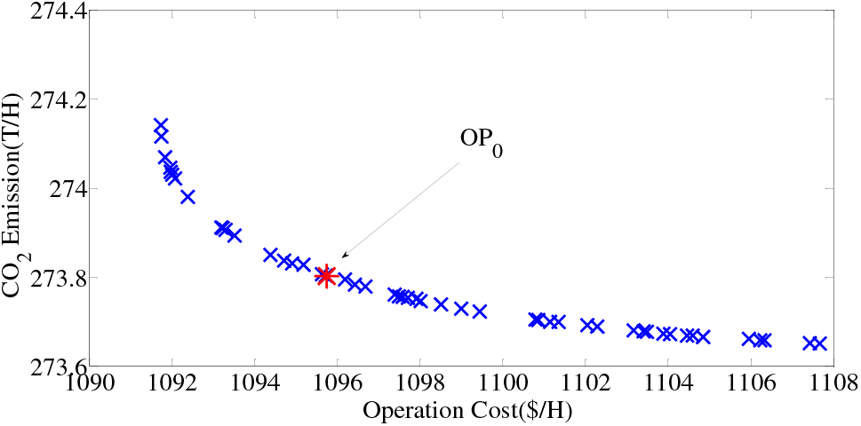
Figure 3: Pareto front of the first optimal stage with β=0.9

There are two contingencies involved in the following TSC consideration, which are the same as in references [31,32].

C1: A three-phase grounding fault occurs at bus 9 and is cleared by tripping line 9–6 after lasting 0.35 s which is longer than the critical clearing time (CCT) [32].

C2: A three-phase grounding fault occurs at bus 7 and is cleared by tripping line 7–5 after lasting 0.45 s which is also longer than the CCT [32].

The TDS trajectory of the initial operation point OP0 under contingency C1 and C2 separately can be seen in Fig. 4 which shows that the initial optimal scheme OP0 before generation re-dispatch makes the system unstable when any of the contingencies occurs.

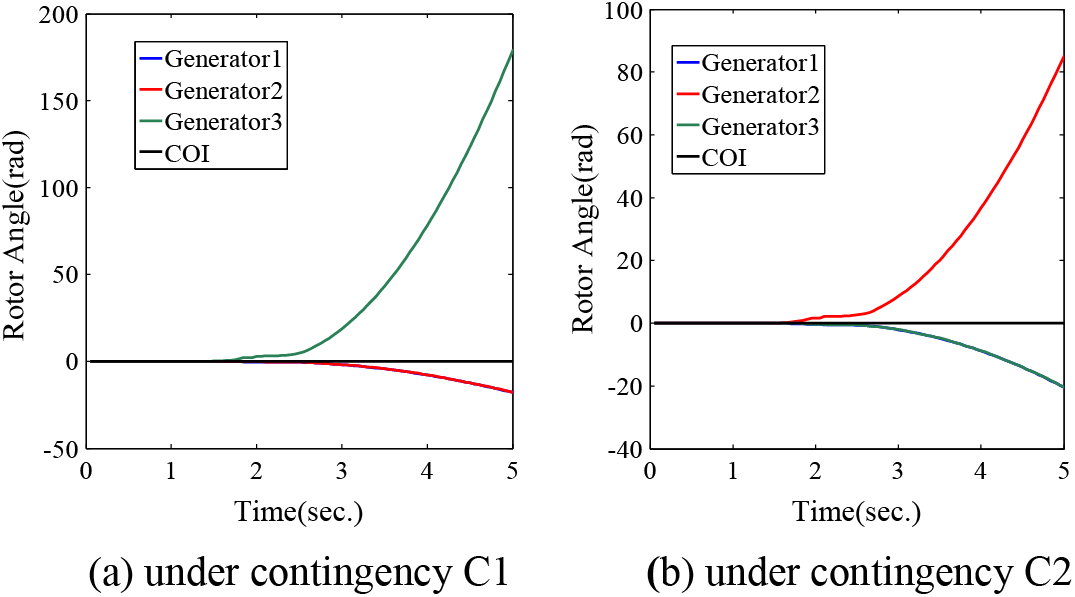
Figure 4: Unstable rotor angle trajectory of initial operation point OP0 of the 30 MW-wind-farm connected WCSS system

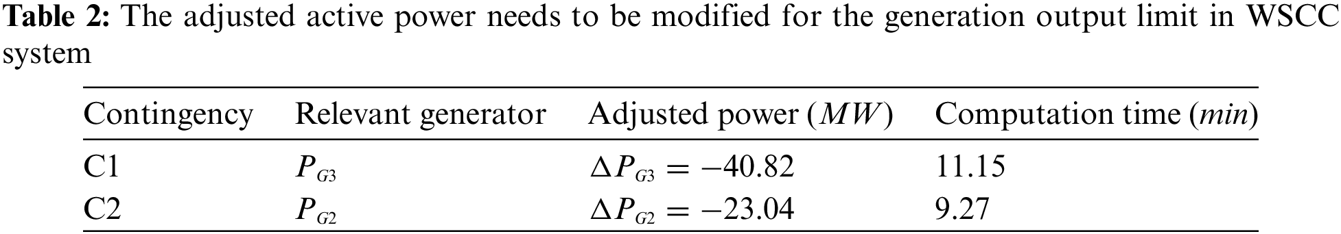
The result of the second optimization stage which conducts the transient stability (TS) security region searching on the base of OP0 is displayed in Table 2.

The Pareto fronts in the first and third optimization stages are compared in Fig. 5 which shows that the Pareto fronts of the optimization concerning the TSC shift to the right and upward no matter for the C1 or the C2 contingency. It is easy to understand that the added transient stability constraint contracts the possible operation region, and results in the increase of optimization objective values. The Pareto front of C1 goes higher and more right than that of C2, and it illustrates that the contingency C1 is more critical than C2 which can also be confirmed by Fig. 3.

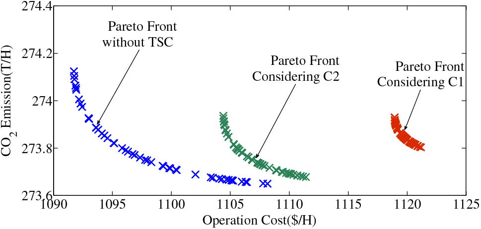
Figure 5: Pareto fronts of 30 MW-wind-farm connected WSCC system with and without TSC

The final PMO-TSCOPF optimal operation schemes OPbest1 and OPbest2 which concern C1 or C2 separately based on the fuzzy membership strategy can be seen in Table 3 and Fig. 6.

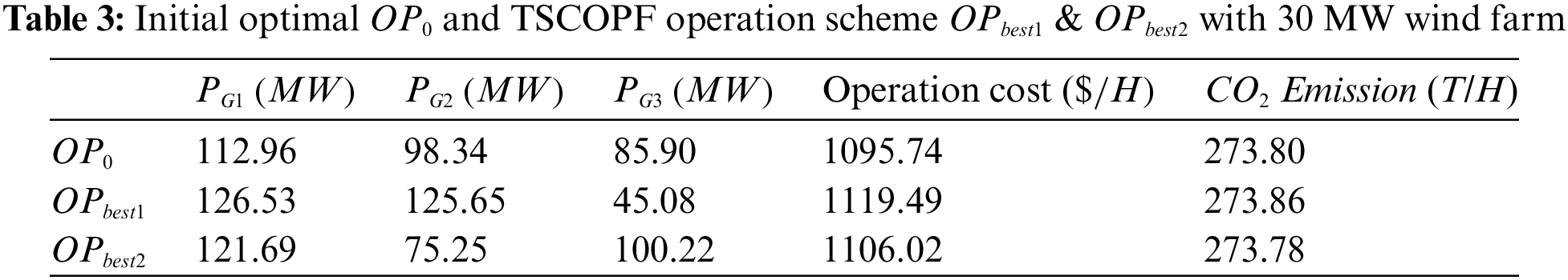
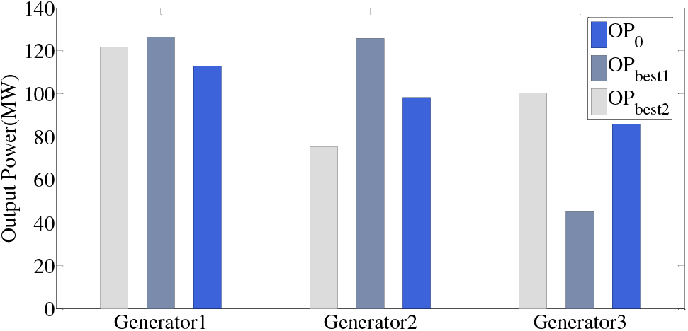
Figure 6: Results comparison with contingency TSC (OPbest1,OPbest2) and without TSC (OP0) of WSCC system connected with 30 MW wind farm

Fig. 6 shows the difference in operating scheme before and after the concern of TSC, and the operating point is pulled to the stable operation region by generation rescheduling. It is obvious that the TSC limits the power production of generators related to certain contingency and therefore the operation feasible region is reduced. So the objective value (which is mainly operation cost) of final optimal results OPbest1, OPbest2 are quite higher than that of initial optimal OP0 due to the restricted feasible solution region. But the re-dispatched operation schedule guarantees the transient stability of the system which can be obviously displayed by the TDS trajectory after faults in Fig. 7.

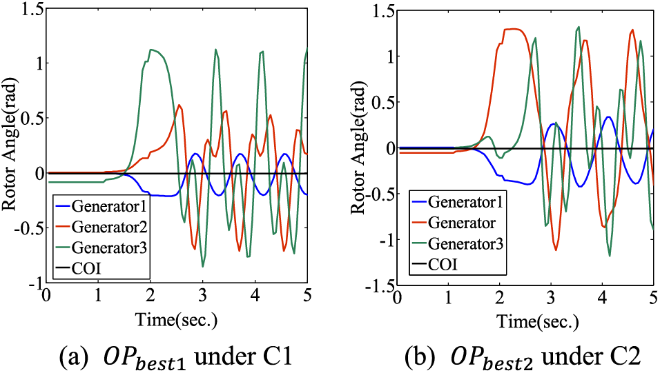
Figure 7: The rotor speed trajectory of final operation schemes under contingency for WCSS 9-bus system with 30 MW wind farm

If the wind farm penetration level increases to 14.3% with the wind farm installation capacity of 45 MW, the initial scheme OP0 and the final operation scheme considering C1 and C2 separately are in Table 4. The calculation time spent on the TS region confirming for C1 and C2 in the second stage are 11.61 and 13.75 min, respectively.

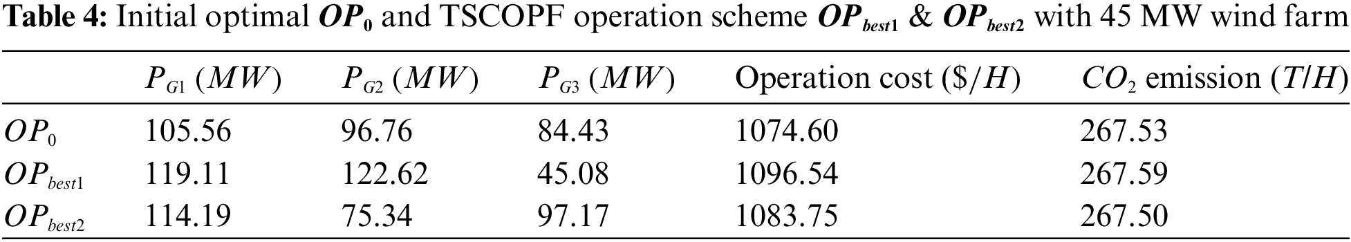
Similarly, the TSC optimal results need higher operation costs for the security requirements in optimization.

Compare the first rows in Tables 3 and 4, and it is easy to understand that the operation cost and pollution gas emission both decrease with the increase of wind generation penetration level because of the lower output of traditional coal-fired generators considering the power balancing.

As for the TSCOPF optimum results in the corresponding rows of the two tables, the data indicate that the wind generation penetration level has a great influence on the TSC optimal result. The larger the wind farm capacity is, the lower relative inertia would be left in the system. This is not beneficial to maintain transient stability which should be theoretically reflected by the worse optimized result. But for the WSCC-9 bus system, the benefit from the increase of wind generation penetration level apparently exceeds the raised cost due to the security restriction.

The optimal results no matter without TSC (OP0) or with TSC (OPbest1,OPbest2) are superior to those in references [31] and [32], which is undoubted for the reason of wind farm integration. As regards probabilistic TSCOPF of wind farm systems, there is little research in existing literatures.

4.2 Modified New England 39-Bus System

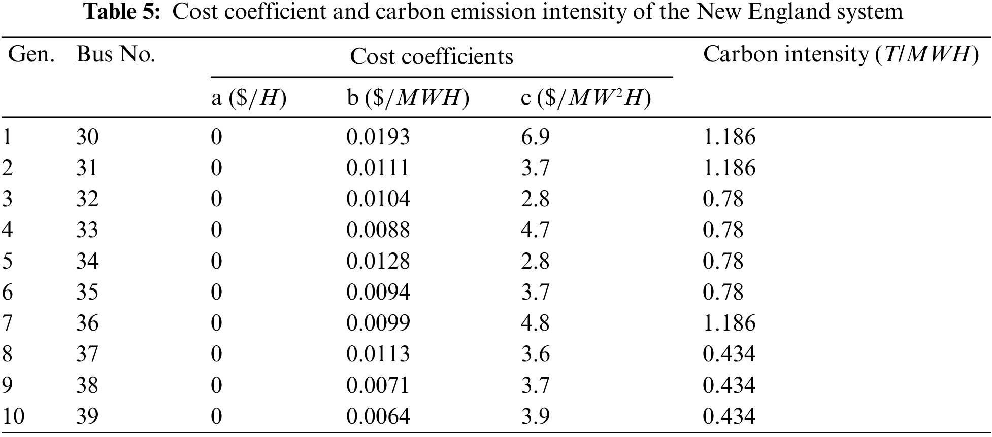
The diagram and information of the original New England 10-machine 39-bus system can be found in the references [31] and [32]. The wind farm is connected to bus 8 in this research and the parameters of the wind turbines and power load are the same as those in Section 4.1. The chance-constraints confidence levels β all equal 0.9; the fuel cost coefficients and carbon emission intensities of synchronous generators are in Table 5 and other settings are based on the MATPOWER case file.

The multi-contingencies are considered in this case, which means the final optimum re-dispatch scheme should ensure the system’s transient stability under any contingency in the fault set when it occurs separately.

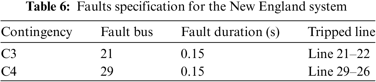
The fault set consists of two three-phase bus faults which are summarized in Table 6 and the fault duration time is greater than the CCT.

The Pareto fronts of the New England system with and without TSC concern are displayed in Fig. 8, which also shows the Pareto fronts with 300 and 600 MW wind farms separately. It can be observed that for different wind generation penetration levels, the Pareto fronts with TSC both go to the right and upward. This is definitely due to the shrink of the feasible solution region. With the increases of wind generation penetration level, the Pareto fronts (with and without TSC) go to the left and downward which means the larger wind farm capacity can provide the system with better operation solutions.

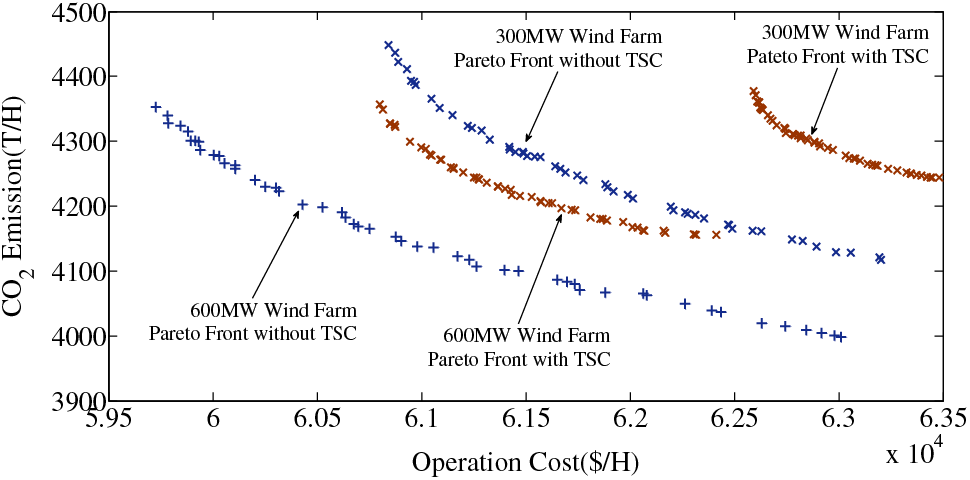
Figure 8: Pareto fronts of the New England system with and without TSC for different wind generation penetrations

The optimal operation schemes without TSC (initial optimal operation point OP0) and with TSC (final optimal operation point OPbest) for 300 or 600 MW wind farm are listed in Table 7.

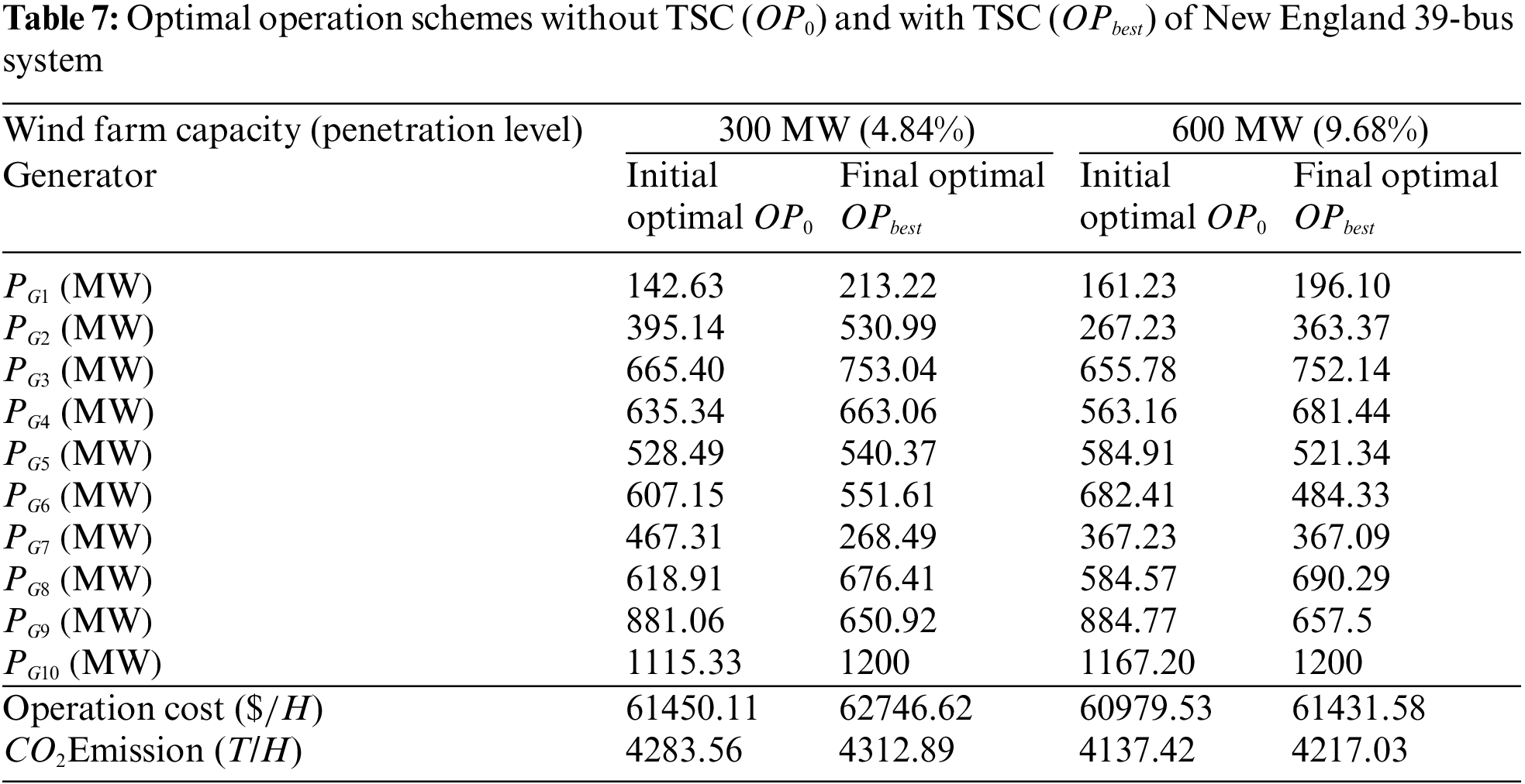
The added objective value from OP0 to OPbest is the cost needed for the restricted TS feasible region and the transient stability of the re-dispatched system can be verified by the simulation as shown in Figs. 9 and 10.

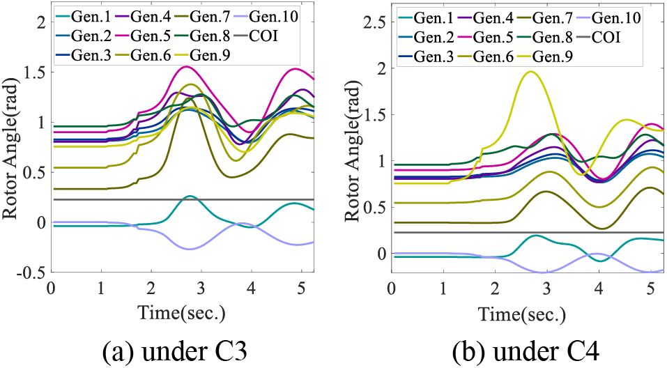
Figure 9: The rotor speed trajectory under contingency at final operation point OPbest of New England system with 300 MW wind farm

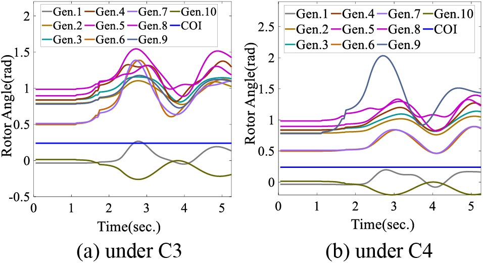
Figure 10: The rotor speed trajectory under contingency at final operation point OPbest of New England system with 600 MW wind farm

The comparison between the final optimization results of different capacity wind farms reveals that for the New England 39-bus system, with the increase of the wind generation penetration level, the PMO-TSCOPF result gets more superior objective values with the consideration of both TSC and uncertainty simultaneously.

In order to validate the ability for searching the most optimal solution of the proposed strategy, the comparison results of the strategy with the existing method as mentioned in reference [6] are shown in Table 8.

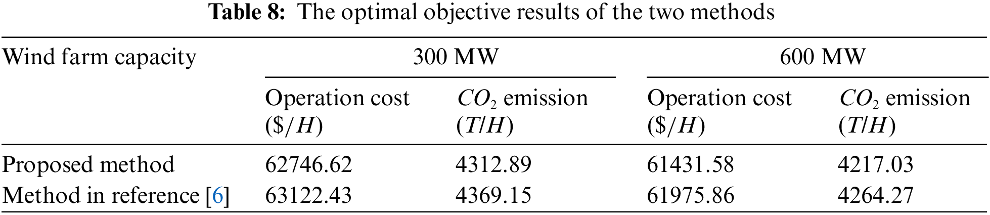
The proposed strategy comes up with the more optimal solution obviously due to the implementation of the third optimization stage. While in the existing method, the re-dispatch scheme is obtained just by shifting the transfer active power from the most advanced generator to the least advanced one to satisfy the transient constraint. It cannot be ensured as the most optimal operation plan due to the lack of an optimization process.

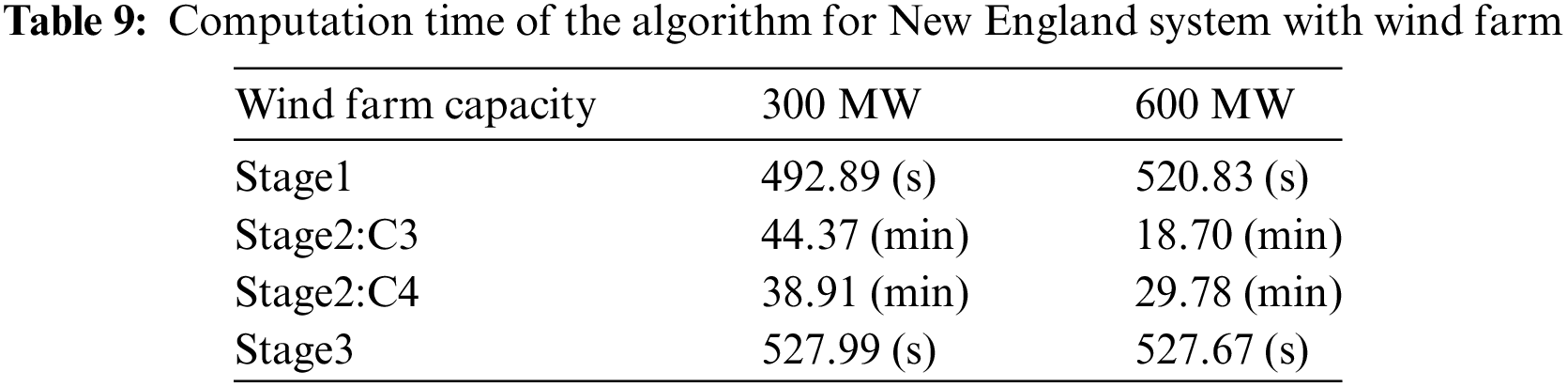
As regards the computational cost for this more complicated system, the execution time is shown in Table 9.

5  Conclusion

In this research, a PMO-TSCOPF framework which consists of three optimization stages is put forward for the wind farm system. Integrating the optimal operation cost & pollution air emission, the chance constraints for uncertain factors, and the transient stability constraints for multi-contingencies into a unified optimization framework and then effectively providing operators with the optimum transient preventive control schemes is the main contribution of this research. The P-MOPSO cooperated with deterministic IPM is utilized as the optimization algorithm.

The numerical results of the strategy on two test systems demonstrate that the TSCOPF optimum re-dispatch scheme brings the increase of multi-objective values compared with the optimal scheme without TSC. This is the cost of the rigorous transient stability constraints for the reduced feasible domain. Furthermore, with the growth of wind generation penetration, the optimum results get superior objective values. This reveals that, although the increased wind farm capacity brings the lower relative inertia left in the system it still results in the reduced output of traditional coal-fired generators and then the decrease in system operation cost and pollution gas emission. In a certain range, the profit of the latter exceeds the cost of the former. The consumption time in the numerical simulations shows that the proposed methodology is suitable for the offline application of transient stability preventive control. Furthermore, this three-stage optimization framework is not dependent on the adopted specific optimization method here; it is flexible to support other optimal algorithms and can be extended to more detailed system modeling.

For further work, how to accelerate the solution speed is the focus of the algorithm in the future.

Acknowledgement: Thanks for the help from Nanjing Institute of Technology.

Funding Statement: The authors received no specific funding for this study.

Author Contributions: The authors confirm contribution to the paper as follows: study conception and design: Yuping Bian; analysis and interpretation of results: Xiu Wan; manuscript revision: Xiaoyu Zhou. All authors reviewed the results and approved the final version of the manuscript.

Availability of Data and Materials: The data used in the study are available from the corresponding author on request.

Conflicts of Interest: The authors declare that they have no conflicts of interest to report regarding the present study.

References

1. Ren, J., Li, B., Zhao, M., Shi, H., You, H. et al. (2022). A fast sequential transient stability preventive control approach driven by model interpretation. Electric Power Systems Research, 213(2022), 1–11. [Google Scholar]

2. Pizano-Martinez, A., Fuerte-Esquivel, C. R., Ruiz-Vega, D. (2010). Global transient stability-constrained optimal power flow using SIME sensitivity analysis. IEEE PES General Meeting, pp. 1–8. Minneapolis, MN, USA. [Google Scholar]

3. Geng, G., Jiang, Q. (2012). A two-level parallel decomposition approach for transient stability constrained optimal power flow. IEEE Transactions on Power Systems, 27(4), 2063–2073. [Google Scholar]

4. Xu, Y., Chi, Y., Yuan, H. (2023). Stability-constrained optimization for modern power system operation and planning. USA: John Wiley & Sons, Wiley-IEEE Press. [Google Scholar]

5. Xia, S., Ding, Z., Shahidehpour, M., Chan, K., Bu, S. et al. (2020). Transient stability-constrained optimal power flow calculation with extremely unstable conditions using energy sensitivity method. IEEE Transactions on Power Systems, 36(1), 355–365. [Google Scholar]

6. Xiang, Y., Liu, Y., Yang, J., Yang, W. (2016). A chance-constrained optimization model for determining renewables penetration limit in power systems. Electric Power Components and Systems, 44(7), 701–712. [Google Scholar]

7. Villegas, C., Ríos, M. A. (2018). Probabilistic contingency severity index for dynamic reactive power planning. 2018 IEEE PES Transmission & Distribution Conference and Exhibition-Latin America, pp. 1–5. Lima, Peru. [Google Scholar]

8. Xia, S., Luo, X., Chan, K. W., Zhou, M., Li, G. (2016). Probabilistic transient stability constrained optimal power flow for power systems with multiple correlated uncertain wind generations. IEEE Transactions on Sustainable Energy, 7(3), 1133–1144. [Google Scholar]

9. Lotfi, H., Ghazi, R. (2021). Optimal participation of demand response aggregators in reconfigurable distribution system considering photovoltaic and storage units. Journal of Ambient Intelligence and Humanized Computing, 12, 2233–2255. [Google Scholar]

10. Lotfi, H. (2020). Multi-objective energy management approach in distribution grid integrated with energy storage units considering the demand response program. International Journal of Energy Research, 44(13), 10662–10681. [Google Scholar]

11. Tang, Y., Luo, C., Yang, J., He, H. (2017). A chance constrained optimal reserve scheduling approach for economic dispatch considering wind penetration. IEEE/CAA Journal Automatica Sinica, 4(2), 186–194. [Google Scholar]

12. Huang, Y., Wang, L., Guo, W., Kang, Q., Wu, Q. (2016). Chance constrained optimization in a home energy management system. IEEE Transactions on Smart Grid, 9(1), 252–260. [Google Scholar]

13. Zhang, H., Lai, C. S., Xu, F., Lai, L. L. (2016). Comparison between probabilistic optimal power flow and probabilistic power flow with carbon emission consideration. 2015 IEEE International Conference on Systems, Man, and Cybernetics, pp. 647–652. Hong Kong, China. [Google Scholar]

14. Basu, M. (2014). Fuel constrained economic emission dispatch using no dominated sorting genetic algorithm-II. Energy, 78, 649–664. [Google Scholar]

15. Morales, J. D., Milanović, J. V., Papadopoulos, P. N. (2019). Analysis of angular threshold criteria for transient instability identification in uncertain power systems. IEEE PowerTech Conference, pp. 1–6. Milan, Italy, IEEE. [Google Scholar]

16. Xin, H., Gan, D., Huang, Z., Zhuang, K., Cao, L. (2010). Applications of stability-constrained optimal power flow in the east china system. IEEE Transactions on Power Systems, 25(3), 1423–1433. [Google Scholar]

17. Milano, F. (2008). PSAT: Power system analysis toolbox documentation for PSAT version 2.0.0. http://faraday1.ucd.ie/software.html (accessed on 01/11/2023). [Google Scholar]

18. Yu, J., Qi, H., Qiu, S., Wang, X., Zhang, H. (2016). Probabilistic load flow calculation with irregular distribution variables considering power grid receivability of wind power generation. The 8th International Power Electronics and Motion Control Conference, pp. 1457–1461. Hefei, China. [Google Scholar]

19. Ruiz-Rodriguez, F. J., Hernandez, J. C., Jurado, F. (2012). Probabilistic load flow for radial distribution networks with photovoltaic generators. IET Renewable Power Generation, 6(2), 110–121. [Google Scholar]

20. Tian, F., Zhou, X., Yu, Z. (2018). Optimization method of transient stability preventive control based on sensitivity analysis and time domain simulation. Electric Power Automation Equipment, 38(7), 155–161. [Google Scholar]

21. Byrd, R. H., Gilbert, J. C., Nocedal, J. (2000). A trust region method based on interior point techniques for nonlinear programming. Mathematical Programming, 89(1), 149–185. [Google Scholar]

22. Alhazmi, M., Dehghanian, P., Wang, S., Shinde, B. (2019). Power grid optimal topology control considering correlations of system uncertainties. IEEE Transactions on Industry Applications, 55(6), 5594–5604. [Google Scholar]

23. Abido, M. A. (2011). Multiobjective particle swarm optimization for optimal power flow problem. In: Handbook of swarm intelligence: Concepts, principles and applications, pp. 241–268. German: Springer Science & Business Media. [Google Scholar]

24. Metweely, K. M., Morsy, G. A., Amer, R. A. (2017). Multi-objective optimal power flow of power system with FACTS devices using PSO algorithm. 19th International Middle East Power Systems Conference, pp. 1248–1257. Menoufia, Egypt. [Google Scholar]

25. Zhang, H., Li, G., Wang, S. (2022). Optimization dispatching of isolated island microgrid based on improved particle swarm optimization algorithm. Energy Reports, 8, 420–428. [Google Scholar]

26. Clerc, M. (1999). The swarm and the queen: Towards a deterministic and adaptive particle swarm optimization. Proceedings of the 1999 Congress on Evolutionary Computation-CEC99, pp. 1951–1957. Washington, USA. [Google Scholar]

27. Zhu, S., Chen, C., Tian, Y. (2019). Optimization of chaotic multi-objective particle swarm with hybrid mutation and time-varying inertia. Statistics & Decision, 524(8), 13–17. [Google Scholar]

28. Xu, Y., Dong, Z. Y., Meng, K., Zhao, J. H., Wong, K. P. (2012). A hybrid method for transient stability-constrained optimal power flow computation. IEEE Transactions on Power Systems, 27(4), 1769–1777. [Google Scholar]

29. Zimmerman, R. D., Murillo-Sánchez, C. E., Thomas, R. J. (2011). MATPOWER steady-state operations, planning and analysis tools for power systems research and education. IEEE Transactions on Power Systems, 26(1), 12–19. [Google Scholar]

30. Milano, F. (2005). An open source power system analysis toolbox. IEEE Transactions on Power Systems, 20(3), 1199–1206. [Google Scholar]

31. Nguyen, T. B., Pai, M. A. (2003). Dynamic security constrained rescheduling of power systems using trajectory sensitivities. IEEE Transactions on Power Systems, 18(2), 848–854. [Google Scholar]

32. Cai, H. R., Chung, C. Y., Wong, K. P. (2008). Application of differential evolution algorithm for transient stability constrained optimal power flow. IEEE Transactions on Power Systems, 23(2), 719–728. [Google Scholar]