Short-Term Household Load Forecasting Based on Attention Mechanism and CNN-ICPSO-LSTM

1  Introduction

Electricity load forecasting involves using statistics, machine learning, and other methodologies to predict future changes in load by analyzing existing electricity consumption data [1]. Accurate prediction of residential load is especially vital as it provides dependable data for the power system [2]. Firstly, it facilitates effective planning of power grid construction and transformation based on the projected results, leading to reduced investment and operational costs. Secondly, precise prediction of residential load allows for anticipating future load trends and assessing the potential controllable load on the residential side. This is critical for achieving demand response and plays a pivotal role in optimizing control strategies for residential power consumption.

Currently, there exist various methods for load forecasting, typically categorized into traditional statistical methods and advanced machine learning techniques [3,4]. Traditional statistical methods encompass approaches such as the autoregressive integrated moving average (ARIMA) model, exponential smoothing, Kalman filtering, and others [5]. ARIMA is widely used for analyzing and predicting time series data. It usually establishes an autoregressive model by analyzing trends, cycles, and randomness within the dataset [6,7]. Exponential smoothing assigns varying weights to historical data to project future values [8,9]. Moreover, Kalman filtering is a recursive filtering technique grounded in Bayesian theory. It continuously compares predicted values with actual observations, consistently updating the predicted values and covariance matrix to refine the prediction accuracy [10,11].

However, while the aforementioned methods are simple and practical, they place stringent demands on raw data processing and the stability of time series. Furthermore, their effectiveness in capturing nonlinear influencing factors is limited, making them more suitable for scenarios with fewer influencing factors. Modern machine learning methods exhibit proficiency in addressing nonlinear problems and offer greater advantages in short-term load forecasting performance. These methods encompass the expert system approach, support vector machine (SVM), and artificial neural network (ANN) [12]. Among these, the expert system is suitable when data is limited or absent, but it requires designing numerous rules and operates solely within existing knowledge [13,14]. The SVM can achieve commendable performance with restricted data. However, it can be sluggish in handling large-scale training samples and demonstrates reduced prediction efficiency with substantial prediction data [15,16]. Due to the constraints of these two methods, they are rarely used for short-term load forecasting. Although ANNs have good performance in dealing with non-linear problems in load data, due to the unsatisfied ability to learn the temporal features, they may result in relatively low prediction accuracy.

In recent years, the deep learning method derived from ANNs has garnered significant attention due to its high data processing ability, making it a popular approach in the field of load forecasting [17,18]. This method allows for the extraction of internal rules within the data, enabling representation learning. Among these methods, the recurrent neural network (RNN) is capable of dynamically learning from fluctuating data through its cyclic structure [19]. However, it faces limitations such as the vanishing and exploding gradient problem when processing long data sequences. To address this issue, the LSTM network is introduced [20]. Zhang et al. [21] employed the LSTM method to solve the gradient vanishing problem of RNN and improve prediction accuracy. Nevertheless, LSTM also faces challenges when processing long input data sequences, as it can lose sequence information and hinder the construction of structural relationships between data, ultimately impacting prediction accuracy. Conversely, the convolutional neural network (CNN) model is proficient in extracting features from data and accurately processing nonlinear sequences [22]. Therefore, increasing attention is being given to the method of enhancing the accuracy of household load forecasting by incorporating time series analysis and deep learning. Al-Ja’afreh et al. [23] proposed a combined prediction model integrating CNN and LSTM. CNN was utilized to extract features from the data, followed by LSTM for load prediction. This combination model could effectively address the limitation of a single prediction model in dealing with complex features in the data. Furthermore, Wan et al. [24] introduced the attention mechanism to the CNN-LSTM combined prediction model. It allocated attention to key information by assigning probabilities, highlighting the influence of important data and thereby enhancing the model’s accuracy. The attention mechanism optimizes the output of LSTM, preventing information loss caused by excessively long sequences. Additionally, the method of randomly assigning weights is replaced by probability allocation, resulting in higher prediction accuracy.

Although the aforementioned studies have improved the accuracy of predictions through combined prediction methods, they have overlooked the influence of parameter settings in LSTM on prediction accuracy. In reality, the number of neurons and other parameters have a significant impact on prediction accuracy, and manually adjusting these parameters can easily miss the optimal combination. Fan et al. [25] proposed a prediction model jointly optimized by particle swarm optimization (PSO) and LSTM. By optimizing LSTM parameters through PSO, the prediction accuracy of LSTM was enhanced. However, the model’s complexity increased correspondingly, leading to longer running times. Furthermore, the optimization effect of the basic PSO was limited, with the optimization degree not being significant enough, thereby calling for further improvements. To overcome this issue, the improved chaotic particle swarm optimization (ICPSO) method has been proposed [26].

In this study, a short-term load forecasting model combining CNN-ICPSO-LSTM and attention mechanism is proposed. This method utilizes CNN to extract effective feature vectors from historical load sequences and, the LSTM network to model and learn the dynamic changes of these features. Following this, the attention mechanism is used to assign different probability weights to LSTM hidden states, thereby enhancing the influence of important information on load demand. Additionally, the parameters are optimized by the ICPSO algorithm for the LSTM network to further improve the prediction efficiency of the model. The model aims to analyze and process household electricity load data by combining multiple forecasting methods with complementary advantages, thereby achieving more accurate prediction values.

2  Principles of Deep Learning Models

2.1 Principle and Structure of CNN

CNN is a deep learning model including convolutional computation and deep structure. It can learn representations and extract higher-order features from input information. By utilizing local connections and weight sharing, CNN processes the original data more deeply and abstractly, leading to more effective extraction of features.

The structure of CNN is shown in Fig. 1, which primarily consists of multiple convolutional layers, pooling layers, and fully connected layers. Among them, the convolutional layer plays a vital role in extracting data features, with the convolutional kernel responsible for extracting the corresponding data features. The more convolutional kernels there are, the more abstract features will be extracted. The pooling layer is primarily used to reduce the number of irrelevant features and simplify the model’s complexity. The purpose of the fully connected layer is to transform the pooled data into a one-dimensional vector form, making it easier to process the data.

Figure 1: Structure of CNN

2.2 Principle and Structure of LSTM

The LSTM network is an improved version of the RNN model. It adds multiple gates, especially the setting of forget gates. These gate structures enable LSTM to process and remember longer sequences of time series data effectively. They allow the model to filter out irrelevant information from previous time steps, retaining crucial information while discarding less important details. This overcomes the issues of vanishing and exploding gradients typically encountered in traditional networks, and efficiently stores relevant information through the addition of memory units. The LSTM model exhibits strong generalization capabilities, displaying effective learning even when dealing with large or small datasets, and excels at solving nonlinear problems. The gate structure in the LSTM model enables the deletion or addition of information to the cell state. Each gate acts as an optional mechanism that controls the information flow, and its activation is primarily determined by the sigmoid function and dot product operation. The basic cell structure of the LSTM model is shown in Fig. 2.

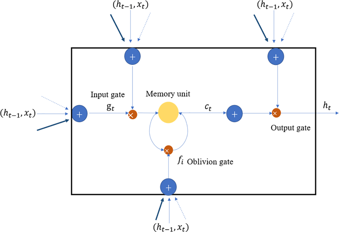
Figure 2: Structure of LSTM network

The LSTM model consists of three gate structures: the forget gate, the input gate, and the output gate. The forget gate is primarily used to regulate the selection of memory information from the previous time step and the current input information. The memory unit utilizes the sigmoid function to filter the memory information, allowing all information to pass when the value is 1, and filtering out all information when the value is 0. This mechanism helps the LSTM model retain important information while disregarding irrelevant information, preventing overfitting. In addition to the forget gate, LSTM also includes the input gate and the output gate. The input gate controls the update of the cell state with new input information. The input information is filtered through the sigmoid function and scaled using the tan⁡h function to ensure that it falls within the range of −1 to 1. The output gate is responsible for generating output based on the current cell state and also utilizes the sigmoid function and tan⁡h function to filter and scale the cell state.

The calculation details of LSTM are as follows. The forget gate can be described by Eq. (1).

fi=sigmoid(wf[ht,xt]+bf)(1)

where fi represents the amount of information passed.

The input gate is shown in Eqs. (2) and (3).

gt=sigmoid(wi[ht−1,xt]+bi)(2)

C~t=tanh⁡(wc[[ht−1,xt]+bc])(3)

The memory unit (information transmission) Ct is shown in Eq. (4).

Ct=Ct−1ft+itCt(4)

The output gate Ot is shown in Eqs. (5) and (6).

Ot=sigmoid(w0[ht−1,xt]+b0)(5)

ht=Ot∗tanh⁡(Ct)(6)

In Eqs. (1)–(6), wf, wi, wc, w0 are the weight indicators, and bf, bi, bc, b0 are the offsets.

2.3 Principle and Structure of the Attention Mechanism

The attention mechanism is a resource allocation mechanism that simulates the human brain’s attention. It allows the model to focus its attention on the most important part of the input data while disregarding the unimportant parts. By calculating the relationship between the input and output of the LSTM hidden layer, the attention mechanism generates a weight vector that represents the importance of each input at the current moment. This weight vector is then used to compute the weighted input vector, which in turn generates the attention output. The core idea behind attention is to combine the output vectors of the LSTM with the vectors in the input sequence, enabling the model to prioritize important information in the input sequence. In the attention mechanism, each vector of the input sequence is assessed for similarity with the LSTM hidden layer output, generating a probability distribution that denotes the significance of each input. This probability distribution can be computed using the softmax function. Through probability allocation, the attention mechanism ensures that enough attention is given to crucial information, emphasizing the impact of important details and thereby enhancing the model’s accuracy. Additionally, the attention mechanism effectively mitigates information loss in LSTM caused by excessively long sequences, while also replacing the previous random weight allocation method with probability allocation.

The structure of the attention mechanism is illustrated in Fig. 3. xt (where t∈[1,n]) represents the input to the LSTM network. ht corresponds to the output of the hidden layer obtained by each input through the LSTM. αt is the probability distribution value of the attention output from the LSTM’s hidden layer through the attention mechanism. y represents the LSTM output value which incorporates the attention mechanism.

Figure 3: Structure of the attention mechanism

3  CNN-ICPSO-LSTM Model Based on Attention Mechanism

3.1 Modeling of ICPSO Optimization Algorithm

In this study, the ICPSO algorithm is utilized to enhance the optimization speed of LSTM and further improve the model’s accuracy. This optimization is carried out during the training process of the prediction model. In each iteration of the ICPSO algorithm, superior particles are stored in the elite database. The fastest descent method is employed to quickly identify values that are close to the optimal solution, thereby preventing premature convergence of the algorithm. This approach aims to enhance the efficiency and effectiveness of the optimization process.

In this algorithm, the position of any particle Xk=[xk1,⋅⋅⋅,xkj,⋅⋅⋅,xkJ]T represents a potential solution to an optimization problem. K particles constitute a population that explores the solution space of the problem. During each iteration, the position of every particle is updated using the following equations:

Vk=ω⋅Vk+c1⋅rand1⋅(Pbestk−Xk)+c2⋅rand2⋅(Gbestk−Xk)(7)

Xk=Vk+Xk(8)

where Xk represents the position of the kth particle in the space. V represents the velocity of particle k. Pbestk represents the best position of the individual. Gbestk represents the global optimal position. rand1 and rand2 are independent random numbers uniformly distributed in the interval [0,1]. c1 and c2 are acceleration constants. ω is the inertia weight factor.

To prevent particles from clustering around local extreme values and getting trapped in local optima, the ICPSO algorithm maintains a balance between the global and local search capabilities of particles by adjusting the inertia weight.

ω(n)={ωmax−(ωmax−ωmin)×S(n)+ωmax+ωmin2×λi|δ2|≤εωmax−(ωmax−ωmin)×S(n)|δ2|>ε(9)

S(t)=11+e−nNmax(10)

where Nmax represents the maximum number of iterations. n represents the current number of iterations. ωmax and ωmin represents the maximum and minimum values of inertia weight.

The population fitness variance and chaotic perturbation strategy are integrated into the inertia weight transformation of the ICPSO algorithm. The population fitness variance, which represents the entropy between particles, is utilized to evaluate the level of particle agglomeration, which is shown as δ2. When δ2 is greater than the critical value, there is no disturbance; otherwise, the more convergent the particles, the worse the diversity of the population. In this situation, the chaotic disturbance strategy is employed to adjust particle movement, enhance population diversity, and enable particles to escape from local optima.

λi+1=4.0×λi×(1−λi)(11)

where the initial value λ0 is a random value between intervals (0,1).

3.2 Parameter Optimization Process of ICPSO-LSTM

The parameter optimization process of ICPSO-LSTM is illustrated in Fig. 4. The weights and parameters of the LSTM network are optimized using the ICPSO algorithm. Generally, the optimization process can be divided into the following steps:

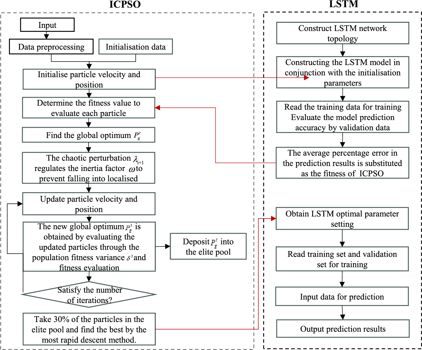
Figure 4: Parameter optimization flowchart of ICPSO-LSTM

(1) The experimental data is divided into training data, validation data, and testing data.

(2) The adaptive ICPSO algorithm is initialized, and the initial LSTM model is constructed based on the parameters associated with each particle in the algorithm. After defining the optimization objective, the model is trained using the training data, and the optimization results are assessed using the validation data. The fitness values of each particle are calculated as the average absolute percentage error of the prediction results. The objective function of the ICPSO algorithm is shown in Eq. (12).

fiti=1n∑i=1n|yi−xixi|(12)

where n represents the total number of predicted values, yi represents the predicted value of the sample, xi represents the actual value.

(3) Update the particle positions using the ICPSO algorithm, and store the updated optimal position values in the elite database. Take 30% of the total number of elite particles in the elite database and optimize these particles using the steepest descent method. The optimization results are then used to update the elite database again. If the iteration limit is reached, substitute the results into the LSTM model for prediction; otherwise, continue with the optimization process.

(4) Output the final optimization results.

3.3 Structure and Modeling of the Prediction Model

The structure of the prediction model is depicted in Fig. 5, comprising an input layer, a CNN layer, an ICPSO-LSTM layer, an attention layer, and an output layer. The model takes historical load data as input, extracts features using the CNN layer, increases feature depth through convolution operations and reduces feature dimensionality via pooling processing. The fully connected layer then converts the features into a one-dimensional structure to complete feature vector extraction. The ICPSO-LSTM layer and the attention layer learn the internal load change patterns from the extracted features to facilitate load prediction. Finally, the load prediction results are obtained through the output layer.

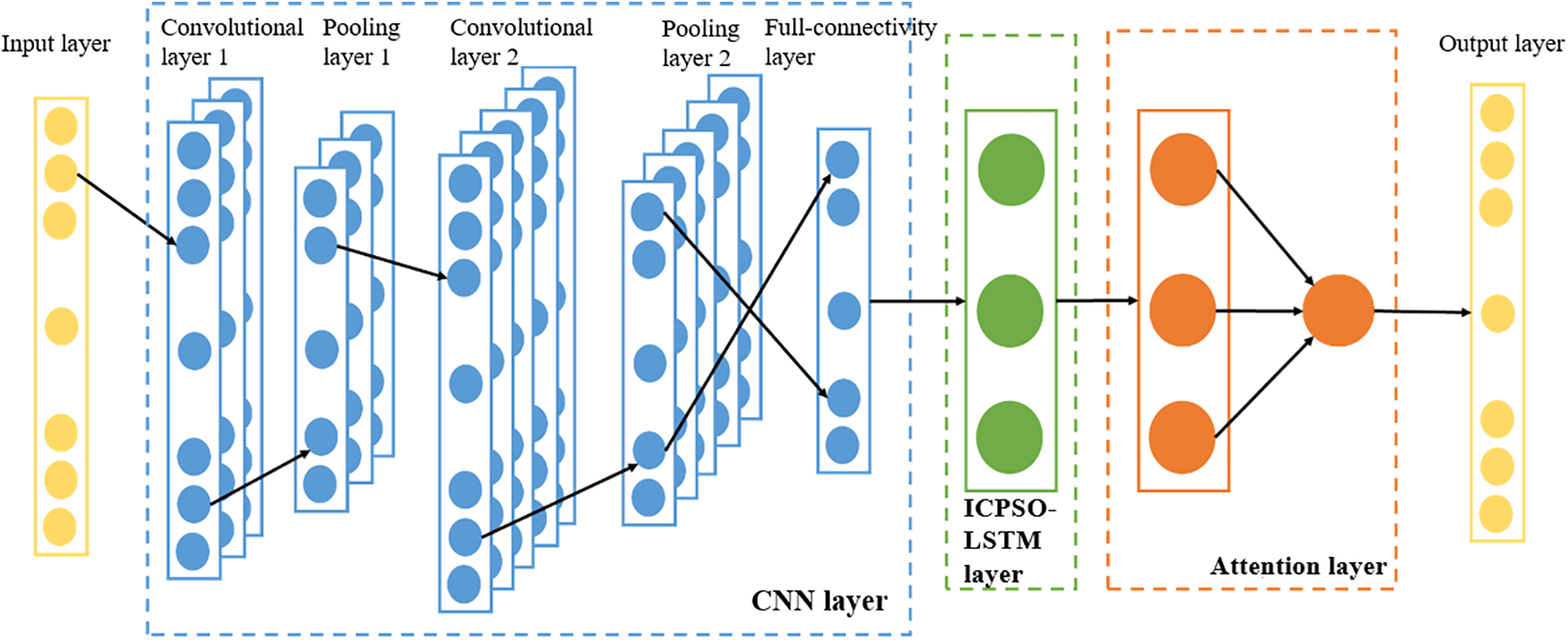
Figure 5: CNN-ICPSO-LSTM model structure based on attention mechanism

Each layer is described in detail as follows:

1) Input layer. The preprocessed historical load data is used as the input layer of the prediction model. The load data has a length of n and is preprocessed before being input into the model, which can be represented by X=[x1⋅⋅,xt−1,xt⋅⋅,xn]T.

2) The CNN layer. The CNN layer is primarily responsible for extracting features from the input historical sequence. The CNN framework consists of two one-dimensional convolution layers, two maximum pooling layers, and one fully connected layer. To accommodate the characteristics of the load data, convolution layers 1 and 2 are designed as one-dimensional convolutions and employ the ReLU activation function. To preserve more fluctuation information in the data, maximum pooling is employed in pooling layers 1 and 2. By processing the convolution and pooling layers, the original data is mapped to the feature space of the hidden layer, and the feature vector is then extracted through the output of the fully connected layer. The fully connected layer uses the Sigmoid activation function. The output feature vector Hc of the CNN layer can be expressed as follows:

Z1=f(X⊗W1+b1)=ReLU(X⊗W1+b1)(13)

P1=max(C1)+b2(14)

Z2=f(P1⊗W2+b3)=ReLU(P1⊗W2+b3)(15)

P2=max(C2)+b4(16)

HC=f(P2⊗W3+b5)=Sigmoid(P2⊗W3+b5)(17)

where Z1 and Z2 are the outputs of convolution layer 1 and convolution layer 2, respectively. P1 and P2 are the outputs of pooled layer 1 and pooled layer 2, respectively. W1, W2 and W3 are the weight matrix. b1, b2, b3, b4 and b5 are deviations. ⊗ and max() are convolution operations and maximum functions. The output length of the CNN layer is i, denoted by Hc=[hc1⋅⋅,hct−1,hct⋅⋅,hci]T.

3) ICPSO-LSTM layer. The ICPSO-LSTM layer is utilized to learn the feature vectors extracted by the CNN layer. The model employs a single-layer LSTM structure to perform deep learning on the extracted feature vector to capture its internal variation pattern. Furthermore, the ICPSO optimization algorithm is employed to optimize the parameters of the LSTM. The output of the ICPSO-LSTM layer is denoted as H, and the output at step t is represented as:

ht=LSTM(HC,t−1,HC,t)(18)

4) Attention layer. The input to the attention mechanism layer is the activated output vector H from the LSTM network layer. By utilizing the principle of weight distribution, the probability of different feature vectors is calculated, and the optimal weight parameter matrix is iteratively determined. The weight coefficient of the attention mechanism layer is computed as follows:

et=μtanh⁡(wht+b)(19)

αt=exp⁡(et)∑t=1iαtht(20)

st=∑t=1iαtht(21)

where et represents the output vector of the LSTM network layer at time t. ht determines the value of the attention probability distribution. μ and w are the weight coefficients. b is the bias coefficient. The output of the attention layer at time t is represented by st.

5) Output layer. The input to the output layer is the output of the attention mechanism layer. The output layer calculates the output Y=[y1,y2⋅⋅⋅ym]T with the predicted step size m through the fully connected layer. The prediction formula can be expressed as:

yt=Sigmoid(w0st+b0)(22)

where yt represents the predicted output value at time t. w0 is the weight matrix, b0 is the deviation vector. The activation function of the Dense layer selects the Sigmoid function.

3.4 Forecasting Process

The flowchart of the forecasting model is shown in Fig. 6. Detailed forecasting process can be illustrated as follows:

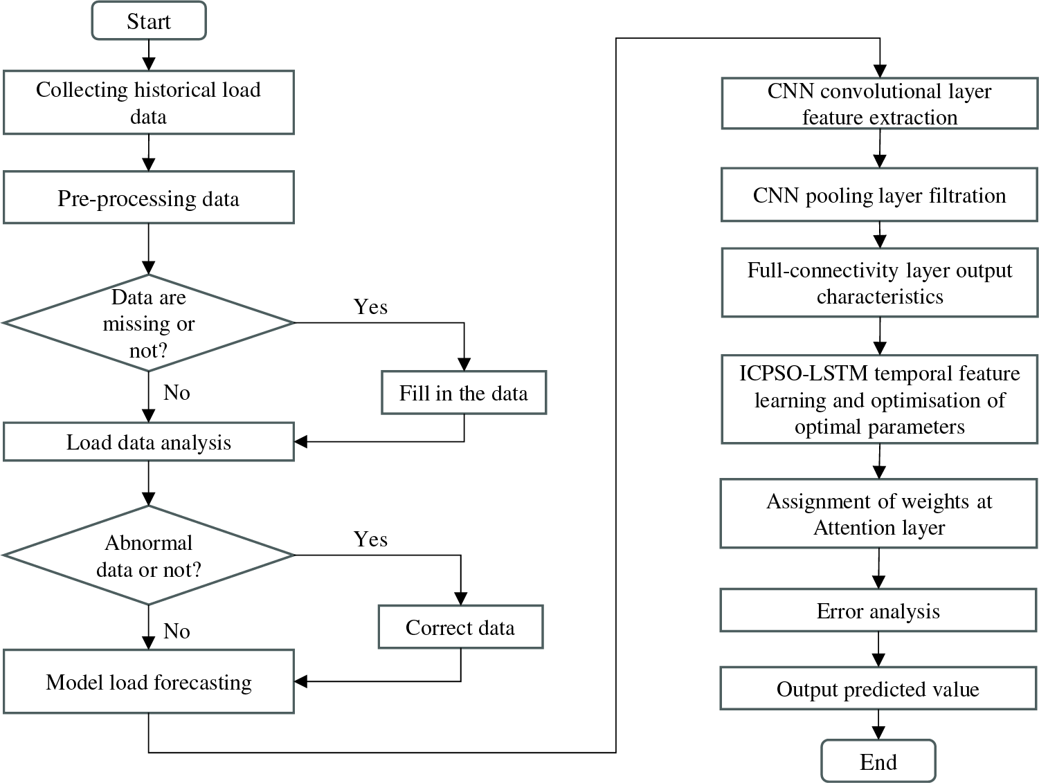
Figure 6: Flow chart of the forecasting model

(1) Data preprocessing: This step involves various tasks, especially noise reduction. In this study, the electricity load data has periodic similarity along the time axis and no continuous mutations, thus the moving average method has been employed for noise reduction. It smooths the data curve by calculating the average value of the data over some time, thereby reducing the impact of noise.

(2) Model training: The data is divided into a training set and a testing set. The training set is used to train the model. The data from the training set is inputted into the model, where the CNN layer performs feature extraction, and the LSTM layer learns the extracted feature vectors. Additionally, the ICPSO algorithm is employed to find optimal parameters for LSTM, thereby enhancing the training speed.

(3) Forecast result output: The attention mechanism determines the weight values for output, and an error analysis is conducted before outputting the load prediction value.

4  Numerical Analysis

4.1 Example Data Preprocessing

The load dataset of a household in Shanghai from January to December in a specific year has been investigated by the local utility company. The dataset consists of 96 data points per day, collected at 15-minute intervals. A subset of the data is chosen for model training and forecasting. Based on the moving average method, the raw data is denoised to smooth the data and prevent the presence of singular points from affecting load forecasting. The specific operation process is as follows:

(1) Calculate the historical average value of the load, as shown in Eqs. (23) and (24).

X¯n,i=1N∑n=1NXn,i(23)

σ2=1N∑n=1N(Xn,i−X¯n,i)2(24)

(2) According to principle 3σ, the authenticity of the data is determined by Eq. (25).

|X¯n,i−Xn,i|>3σiε(25)

where ε is the threshold.

(3) If Eq. (25) is satisfied, it is judged that the data Xn,i is distorted, and the following Eq. (26) is used for weight correction.

X~n,i=α2∑n=1N(Xn,i+1+Xn,i−1)+β4∑n=1NXn,i1,2,3,4+γX¯n,i(26)

where α+β+γ=1, the load correction data on day n is X~n,i. Xn,i−1 and Xn,i+1 are the two nearest lateral multivariate load points, respectively. Xn,i1,2,3,4 is the 4 similar daily multivariate load points near Xn,i.

Moreover, to facilitate the training of the model network, the min-max normalization method is applied to normalize the original data within the range of (−1, 1), using the following calculation formula:

dn=d−dmeandmax−dmin(27)

where d is the original load data. dn is the data after normalization processing. dmean, dmax and dmin are the average, maximum, and minimum values of the sample data, respectively.

4.2 Evaluation Indicators of Forecasting Performance

To assess the accuracy of the model’s predictions, the mean absolute percentage error (MAPE) and root mean square error (RMSE) are employed as evaluation criteria, as shown in Eqs. (28) and (29). MAPE serves as a metric for assessing the quality of the model’s prediction results, while RMSE evaluates the accuracy of the predictions and is sensitive to both large and small errors reflected in the results. When forecasting the electricity load, a smaller value of MAPE and RMSE indicates a more accurate load forecasting result.

MAPE=1n∑i=1n|yi−y¯i|yi×100%(28)

RMSE=1n∑i=1n(yi−y¯i)2(29)

where n represents the total number of predicted results. yi and y¯i are the actual load value and the predicted load value of the sampling point i, respectively.

4.3 Forecasting Results and Analysis

To validate the superiority and reliability of the proposed model for short-term load forecasting, six groups of comparison models are established, including (1) the LSTM method; (2) the CNN-GRU combined prediction method without incorporating the attention mechanism; (3) the CNN-LSTM combined prediction method without incorporating the attention mechanism; (4) CNN-PSO-GRU combined prediction method based on the attention mechanism; (5) CNN-PSO-LSTM combined prediction method based on the attention mechanism; (6) CNN-ICPSO-LSTM combined prediction method based on the attention mechanism; (7) CNN-PSO-BiLSTM combined prediction method based on the attention mechanism; (8) CNN-ICPSO-BiLSTM combined prediction method based on the attention mechanism.

In this study, all computational programs have been run on a laptop computer configured with an Intel Core i7-13700HX processor and 16 G RAM.

4.3.1 Performance Comparison of Different Forecasting Methods

After analyzing the initial load data, it is evident that the household load exhibits clear periodic changes corresponding to seasonal variations, with significant fluctuations during summer and winter. Therefore, the household load data in summer and winter are chosen for prediction and comparison.

To verify the scientificity and stability of the forecasting models, a random week from each season of the dataset is chosen for daily load forecasting. The results of single-day load forecasting may not directly indicate the stability of the forecasting model. Therefore, the daily load forecasting results for seven days per week are analyzed from an average standpoint. The performance indicators of different forecasting models are presented in Table 1.

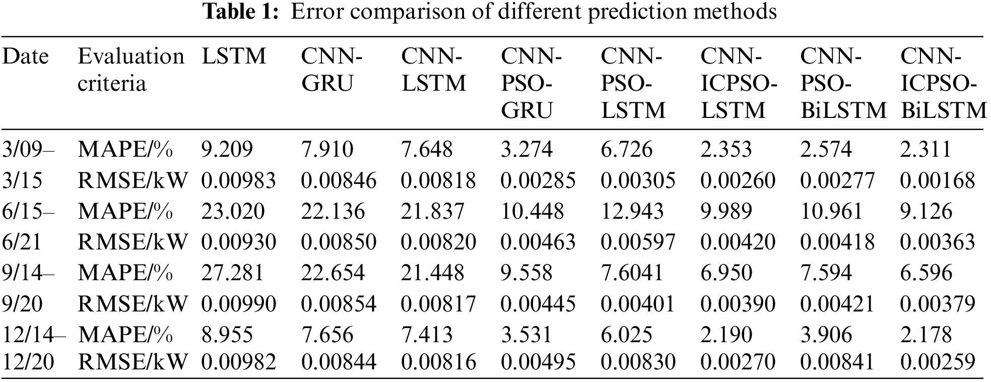
In terms of the error comparison, Table 1 clearly shows that there are significant variations in error comparisons across different seasons. The error is higher in summer and autumn when the load data exhibits high volatility, while the error is lower in spring and winter when the load data is less volatile. This suggests that data volatility also has a significant impact on the model’s prediction results. It is worth noting that MAPE measures the quality of the model’s prediction results. When data fluctuations have a substantial impact, its value will change proportionally with the changes in the prediction results. On the other hand, RMSE assesses the prediction accuracy of the model. When the model operates stably, the prediction accuracy remains relatively consistent.

Moreover, based on the results presented in Table 1, it can be observed that the LSTM model exhibits the highest MAPE and RMSE values, indicating the poorest prediction performance. On the contrary, the proposed model in this study demonstrates the lowest MAPE and RMSE values, signifying a higher overall prediction accuracy. Taking the average prediction error for the period of 6/15–6/21 as an example, compared with the LSTM method, the implementation of the CNN-LSTM model leads to a reduction of 1.18% in MAPE and 11.82% in RMSE. When the PSO algorithm and the attention mechanism are included, the prediction accuracy can be significantly improved for both CNN-PSO-GRU and CNN-PSO-LSTM models. Moreover, when using the ICPSO algorithm instead of the PSO algorithm, the MAPE value of the CNN-ICPSO-LSTM model is reduced by 23.52% compared with the CNN-PSO-LSTM model.

In this study, the proposed CNN-ICPSO-LSTM model utilizes CNN for feature extraction tasks, ensuring the retention of crucial data features, while LSTM is employed to capture the interdependencies among the data. In situations where there are significant load fluctuations, the coupling characteristics among features are leveraged to mitigate prediction errors. Additionally, ICPSO is employed to optimize the LSTM parameters, enabling the identification of the optimal parameter combination and improving the operational efficiency of the model. The attention mechanism further enhances the prediction accuracy by assigning weights that highlight the influence of important features.

To conduct a comprehensive comparison, a typical day in both summer and winter, characterized by significant load fluctuations, is selected to compare the load prediction results using different forecasting methods, as illustrated in Figs. 7 and 8.

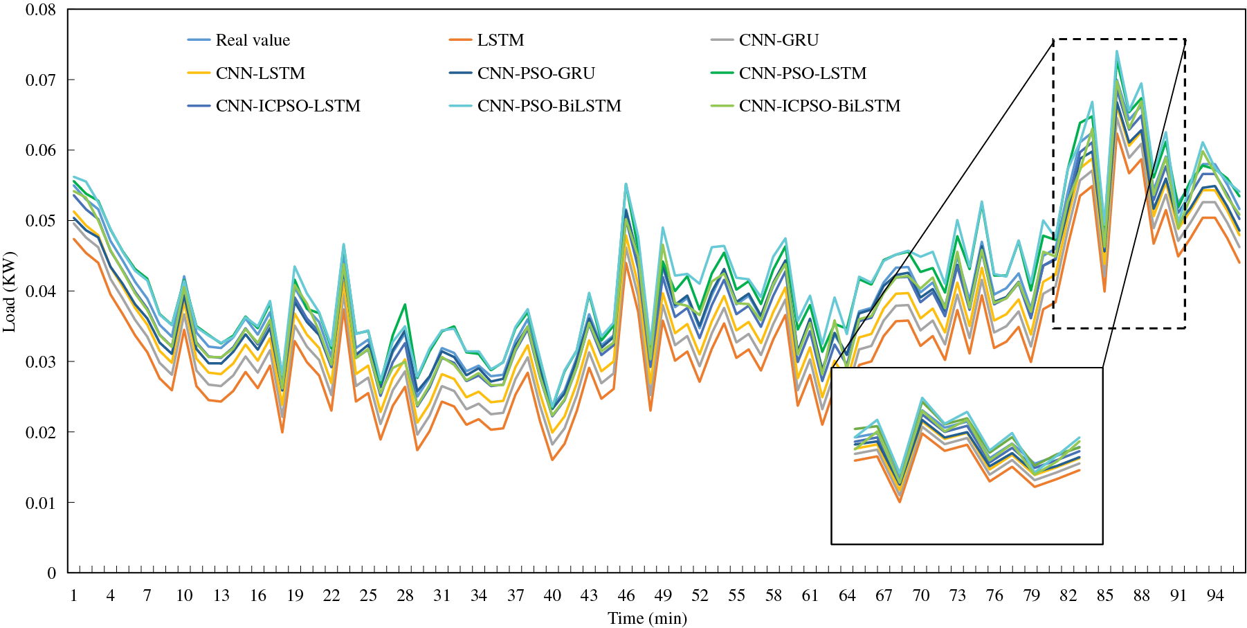
Figure 7: Load forecasting results on a typical summer day

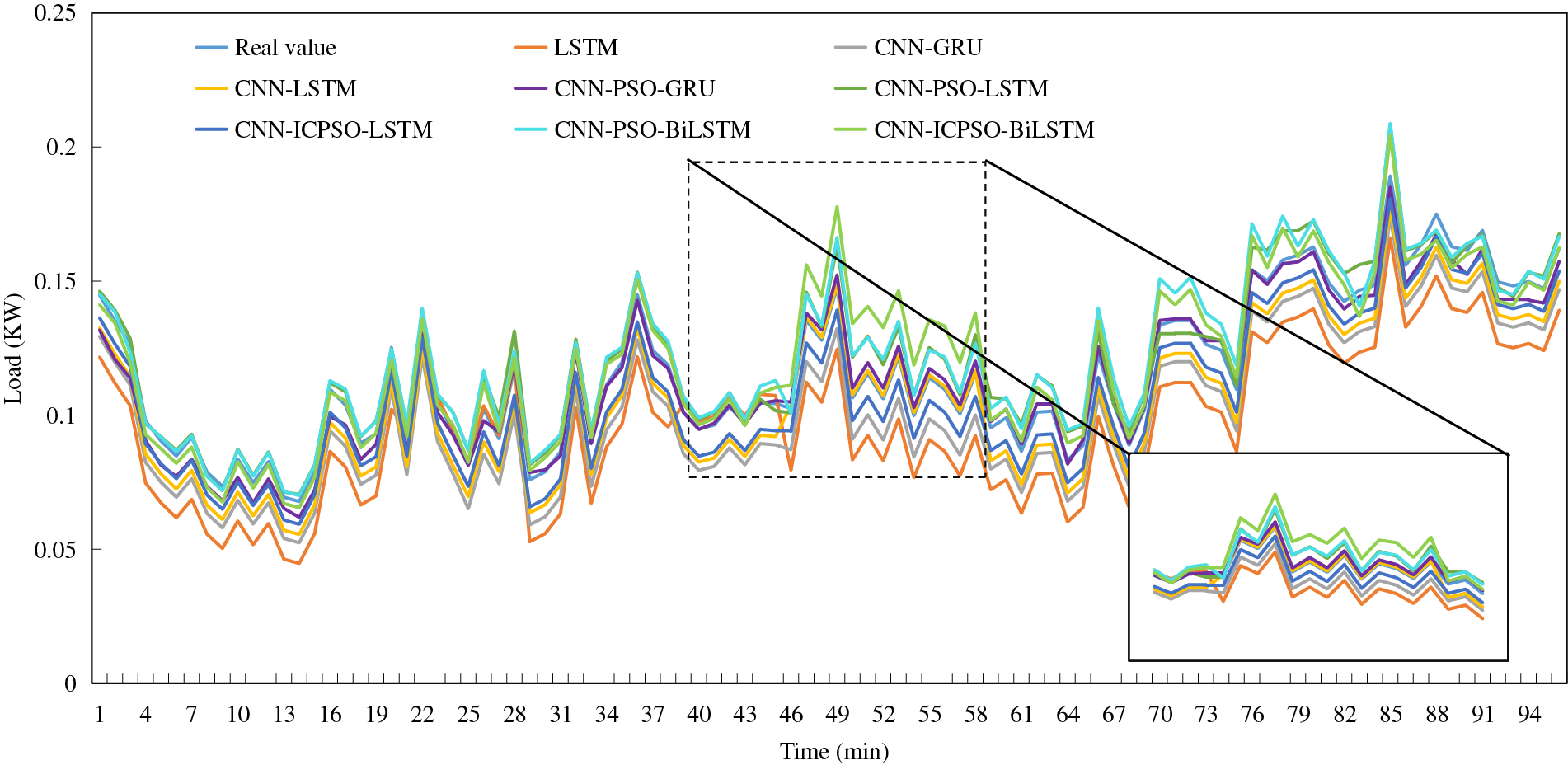
Figure 8: Load forecasting results on a typical winter day

(1) LSTM exhibits a lower fitting degree in comparison to other methods. It is challenging for a single forecasting method to accurately predict load data with substantial fluctuations, and the forecasting results for time series with distinctive characteristics are subpar. Nonetheless, the overall trend of the curve remains relatively consistent with the true values.

(2) There is a minimal disparity between CNN-LSTM and CNN-GRU, both of which exhibit improved fitting degrees and a closer alignment with the true values in terms of the overall trend. This suggests that combined prediction yields higher prediction accuracy compared to individual predictions. Additionally, load forecasting with distinct temporal characteristics outperforms LSTM.

(3) The inclusion of the PSO algorithm improves the prediction accuracy of the original model. Moreover, the application of the ICPSO algorithm makes the above advantages more obvious.

(4) The load trend can be adequately captured by each forecasting model within regions where the load change is relatively steady. However, significant discrepancies between the predicted and actual values are evident in areas characterized by more drastic load changes, particularly in the vicinity of load peaks and troughs.

Generally, in comparison to the other methods, the load forecasting approach proposed in this study demonstrates significantly enhanced fitting degrees. It delivers more accurate predictions for load data with evident time series characteristics, resulting in smaller errors. Moreover, it delivers more accurate predictions for load data with evident time series characteristics, resulting in smaller errors. Moreover, it demonstrates good prediction performance for all typical days with significant different load profiles, demonstrating its satisfied robustness.

In addition, it is interesting to notice that, the predicted values using most models are lower than the true value. It is considered to be a coincidence using specific input data. There is no clear theoretical basis to support the above phenomenon. In addition, it is found that the forecasting accuracy in winter is better than that in summer. This may be due to the greater impact of temperature and humidity on summer loads, resulting in stronger load fluctuations than in winter. This fluctuation increases the difficulty of load forecasting and reduces the prediction accuracy.

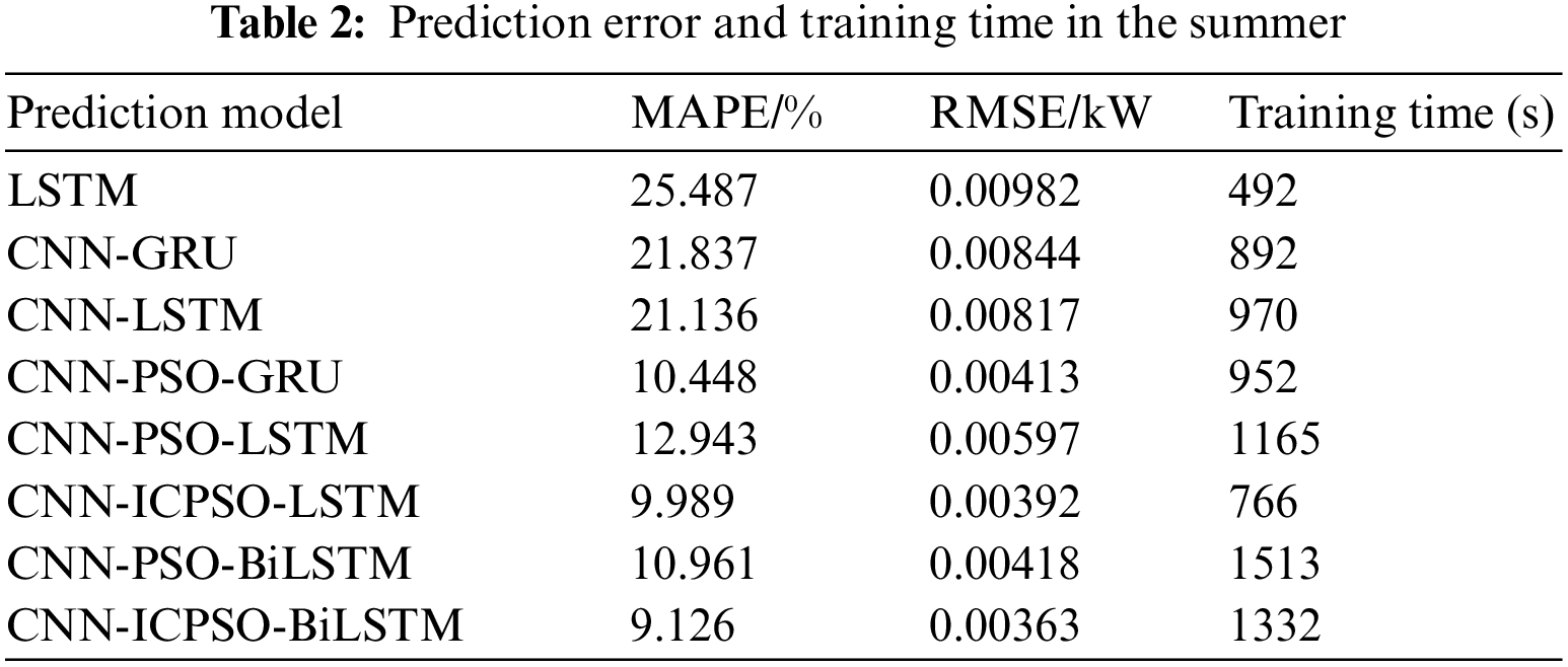
Taking the load prediction results on a typical summer day as an example, the errors and training times of different models are compared and analyzed, as presented in Table 2. The single prediction model exhibits the shortest training time but a larger error compared to the hybrid model due to the absence of feature extraction. Although the training time of CNN-GRU is lower than that of CNN-LSTM, the error is relatively high. The combination of the PSO algorithms can improve the prediction accuracy, but may greatly increase the computation amount. The computation time of CNN-PSO-LSTM and CNN-PSO-GRU is much more than that of CNN-LSTM and CNN-GRU, respectively. However, through the integration of the ICPSO algorithm, the CNN-ICPSO-LSTM proposed in this study not only ensures prediction accuracy but also reduces model training time. This indicates that the inclusion of an improved optimization algorithm can effectively enhance training speed and reduce model running time. Moreover, as an improved version of LSTM, the inclusion of BiLSTM may improve the prediction accuracy to some extent, while resulting in relatively long training time. Therefore, balancing the prediction accuracy and efficiency, CNN-ICPSO-LSTM model combined with attention mechanism may be a good option for the short-term household load forecasting.

4.3.2 Results Analysis of Error Evaluation Index

To provide a clearer explanation of the error results for each model, Fig. 9 illustrates a comparison between the real value (used as the horizontal coordinate) and the predicted value obtained by each model (used as the vertical coordinate). The closer the predicted value distribution is to the center line, the better the prediction effect.

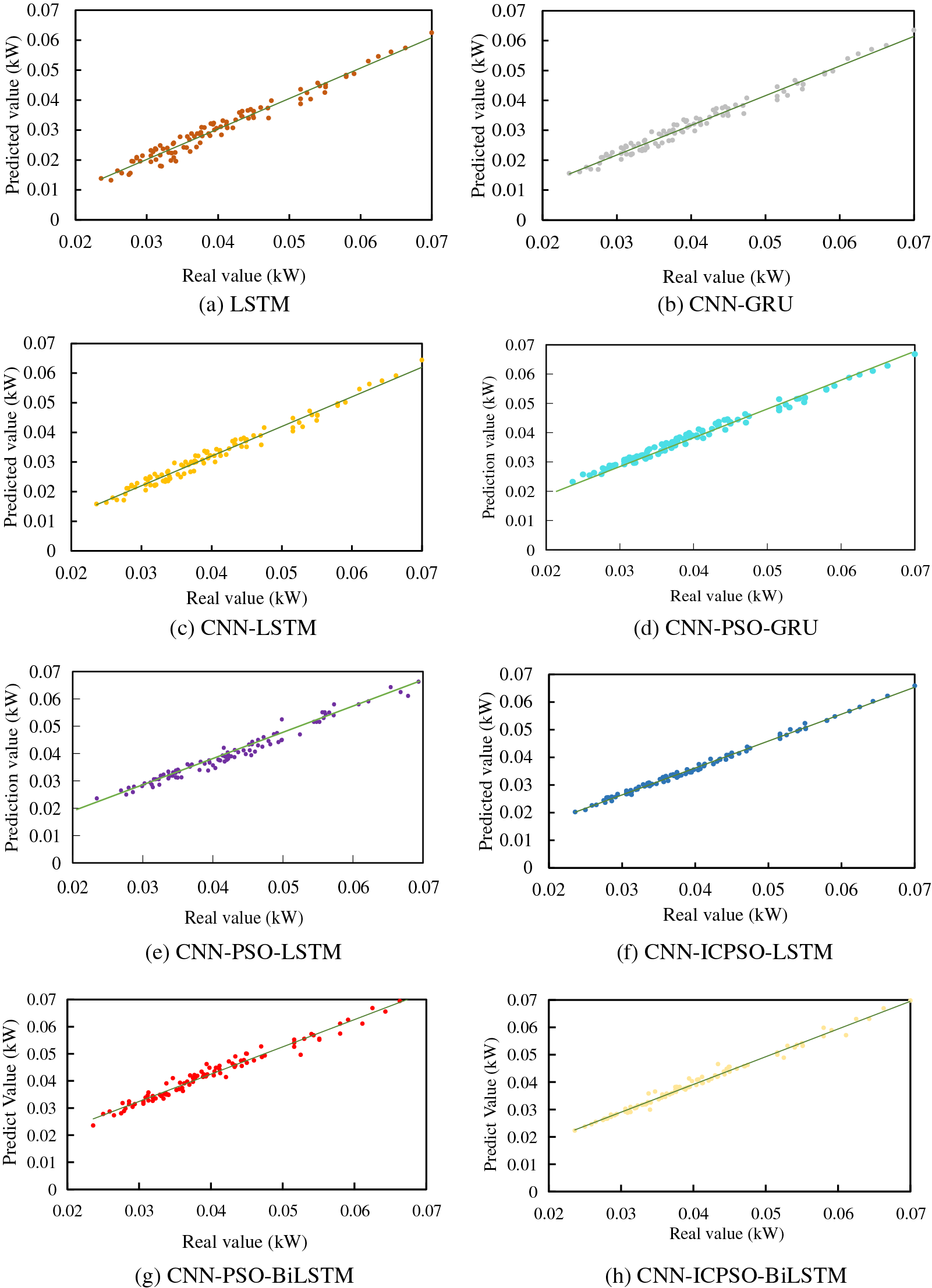
Figure 9: Comparison between predicted results and actual values

As shown in Fig. 9, the six different forecasting methods exhibit varying predicted value distributions. Specifically, the LSTM model, functioning as a standalone forecasting model, displays a more scattered predicted value distribution, suggesting a larger prediction error compared to the other methods. On the other hand, the combined forecasting models of CNN-GRU and CNN-LSTM demonstrate similar predicted value distributions, indicating their prediction errors are relatively comparable and superior to that of the LSTM model. The CNN-PSO-LSTM model and CNN-PSO-GRU model have a more compact distribution compared to the former two, indicating that the latter two models have higher prediction accuracy than the former two. It also indicates that the combination of the PSO algorithm does improve the prediction accuracy. Notably, the proposed prediction model exhibits a more convergent and closer predicted value distribution to the real value in contrast to the other five prediction models. This emphasizes that the prediction results achieved by the proposed model are more realistic and reliable.

4.3.3 Analysis of Long-Term Time Series Prediction Results

The aforementioned analysis confirms that the proposed model exhibits higher accuracy and advantages when dealing the load data with significant fluctuations in different seasons. Additionally, long-term time series prediction results play a vital role in household load prediction. To compare and validate the performance of the six models, load data from three days in both summer and winter are employed. The prediction results of different forecasting models are illustrated in Figs. 10 and 11.

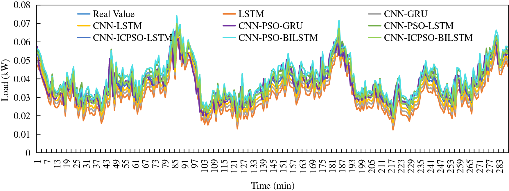
Figure 10: Forecasting results of three days in summer

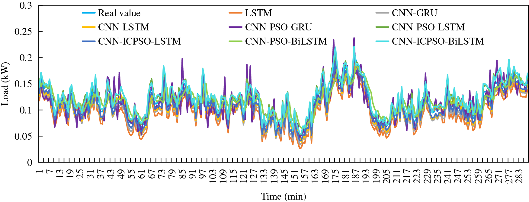
Figure 11: Forecasting results of three days in winter

When extending the forecasting period to 3 days, the proposed method demonstrates a closer alignment with the actual load trend and accurately predicts load fluctuations. It exhibits superior performance during peak and valley periods with significant load variations, accurately analyzing changes in load data at peak and valley values, and showcasing a high level of fitting with the actual load values. As a result, more precise prediction results are achieved.

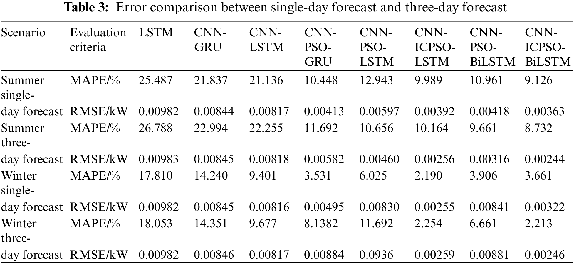
Table 3 shows the comparison of errors between single-day and three-day forecasts. It is evident that as the forecast period extends, the prediction errors for each forecasting model also increase. This indicates that with longer forecast times, the complexity of prediction grows, and subsequently, the prediction accuracy decreases. Considering the results of single-day and three-day forecasts in summer, the average MAPE for other methods increased by 1.301%, 1.119%, 1.157%, 1.224%, and 2.287%, respectively, whereas the average MAPE for the proposed model increased by only 0.175%. This demonstrates that the proposed model can maintain high prediction accuracy and a low error growth rate even with an increased forecast time. This is mainly due to the inclusion of the attention mechanism. It adopts a probability distribution to give sufficient attention to key messages, further compensating for the information loss caused by LSTM due to excessively long sequences.

Based on the aforementioned discussion, the model proposed in this study not only ensures prediction accuracy but also maintains prediction stability. Consequently, it exhibits a strong fitting ability to the actual values. In addition, the model demonstrates high accuracy in both daily and long-term time series prediction, further validating its robustness.

5  Conclusions

To address the challenges posed by the large volume of data for household load forecasting, a hybrid deep learning framework integrating the CNN-ICPSO-LSTM model and the attention mechanism, is proposed for short-term electricity load forecasting. According to the simulation results, the following conclusions can be drawn:

(1) The prediction method proposed in this study not only exhibits significantly lower errors in terms of MAPE and RMSE compared to other prediction methods but also demonstrates a higher degree of curve fitting to the true values in the prediction results. These findings indicate that the proposed method can enhance the accuracy of short-term load forecasting.

(2) The hybrid model exhibits a relatively high level of complexity, resulting in an increased running time compared to a single prediction model. However, compared to the CNN-PSO-GRU and CNN-PSO-LSTM models, the proposed model reduces the overall running time by employing ICPSO to optimize LSTM parameters. This indicates that the proposed method also enhances the training speed of the model.

(3) After increasing the prediction duration, all methods experience an increase in error. However, the method proposed in this study exhibits lower error growth rate, suggesting its capability to predict longer time series with high accuracy.

Acknowledgement: None.

Funding Statement: The research work was supported by the Shanghai Rising-Star Program (No. 22QA1403900), the National Natural Science Foundation of China (No. 71804106), and the Non-carbon Energy Conversion and Utilization Institute under the Shanghai Class IV Peak Disciplinary Development Program.

Author Contributions: The authors confirm contribution to the paper as follows: study conception and design: L. Ma, L. Wang, and H. Ren; data collection: S. Zeng and Y. Zhao; analysis and interpretation of results: C. Liu and H. Zhang; draft manuscript preparation: L. Ma, L. Wang and Q. Wu. All authors reviewed the results and approved the final version of the manuscript.

Availability of Data and Materials: All data, models, or codes that support the findings of this study are available from the corresponding author upon reasonable request.

Conflicts of Interest: The authors declare that they have no conflicts of interest to report regarding the present study.

References

1. Yildiz, B., Bibao, J. I., Sproul, A. B. (2017). A review and analysis of regression and machine learning models on commercial building electricity load forecasting. Renewable and Sustainable Energy Reviews, 73, 1104–1122. 10.1016/j.rser.2017.02.023 [Google Scholar] [CrossRef]

2. Wu, K., Peng, X., Chen, Z., Su, H., Quan, H. et al. (2023). A novel short-term household load forecasting method combined BiLSTM with trend feature extraction. Energy Reports, 9(8), 1013–1022. [Google Scholar]

3. Eren, Y., Küçükdemiral, İ. (2024). A comprehensive review on deep learning approaches for short-term load forecasting. Renewable and Sustainable Energy Reviews, 189, 114031. 10.1016/j.rser.2023.114031 [Google Scholar] [CrossRef]

4. Qian, F., Yue, Y., He, Y., Yu, H., Zhou, Y. et al. (2023). Unsupervised seismic footprint removal with physical prior augmented deep autoencoder. IEEE Transactions on Geoscience and Remote Sensing, 61, 1–20. [Google Scholar]

5. Zheng, Z., Chen, H., Luo, X. (2019). A Kalman filter-based bottom-up approach for household short-term load forecast. Applied Energy, 250, 882–894. 10.1016/j.apenergy.2019.05.102 [Google Scholar] [CrossRef]

6. Tarmanini, C., Sarma, N., Gezegin, C., Ozgonenel, O. (2023). Short term load forecasting based on ARIMA and ANN approaches. Energy Reports, 9(3), 550–557. [Google Scholar]

7. Wu, F., Cattani, C., Song, W., Zio, E. (2020). Fractional ARIMA with an improved cuckoo search optimization for the efficient short-term power load forecasting. Alexandria Engineering Journal, 59(5), 3111–3118. 10.1016/j.aej.2020.06.049 [Google Scholar] [CrossRef]

8. Pritularga, K. F., Svetunkov, I., Kourentzes, N. (2023). Shrinkage estimator for exponential smoothing models. International Journal of Forecasting, 39(3), 1351–1365. 10.1016/j.ijforecast.2022.07.005 [Google Scholar] [CrossRef]

9. Rendon-Sanchez, J. F., Menezes, L. M. (2019). Structural combination of seasonal exponential smoothing forecasts applied to load forecasting. European Journal of Operational Research, 275(3), 916–924. 10.1016/j.ejor.2018.12.013 [Google Scholar] [CrossRef]

10. Owusu, F. K., Amoako-Yirenkyi, P., Frempong, N. K., Omari-Sasu, A. Y., Mensah, I. A. et al. (2023). Seemingly unrelated time series model for forecasting the peak and short-term electricity demand: Evidence from the Kalman filtered Monte Carlo method. Heliyon, 9(8), 18821. 10.1016/j.heliyon.2023.e18821 [Google Scholar] [PubMed] [CrossRef]

11. Takeda, H., Tamura, Y., Sato, S. (2016). Using the ensemble Kalman filter for electricity load forecasting and analysis. Energy, 104, 184–198. 10.1016/j.energy.2016.03.070 [Google Scholar] [CrossRef]

12. Wazirali, R., Yaghoubi, E., Abujazar, M. S. S., Ahmad, R., Vakili, A. H. (2023). State-of-the-art review on energy and load forecasting in microgrids using artificial neural networks, machine learning, and deep learning techniques. Electric Power Systems Research, 225, 109792. 10.1016/j.epsr.2023.109792 [Google Scholar] [CrossRef]

13. Pieroni, M. P. P., Mcaloone, T. C., Borgianni, Y., Maccioni, L., Pigosso, D. C. A. (2021). An expert system for circular economy business modelling: Advising manufacturing companies in decoupling value creation from resource consumption. Sustainable Production and Consumption, 27, 534–550. 10.1016/j.spc.2021.01.023 [Google Scholar] [CrossRef]

14. Roy, S. S., Pratihar, D. K. (2012). Soft computing-based expert systems to predict energy consumption and stability margin in turning gaits of six-legged robots. Expert Systems with Applications, 39(5), 5460–5469. 10.1016/j.eswa.2011.11.039 [Google Scholar] [CrossRef]

15. Samantaray, S., Sahoo, A., Satapathy, D. P. (2022). Improving accuracy of SVM for monthly sediment load prediction using Harris hawks optimization. Materials Today: Proceedings, 61(2), 604–617. [Google Scholar]

16. Aasim, Singh, S. N., Mohapatra, A. (2021). Data driven day-ahead electrical load forecasting through repeated wavelet transform assisted SVM model. Applied Soft Computing, 111, 107730. 10.1016/j.asoc.2021.107730 [Google Scholar] [CrossRef]

17. Fan, G. F., Han, Y. Y., Li, J. W., Peng, L. L., Yeh, Y. H. et al. (2024). A hybrid model for deep learning short-term power load forecasting based on feature extraction statistics techniques. Expert Systems with Applications, 238, 122012. 10.1016/j.eswa.2023.122012 [Google Scholar] [CrossRef]

18. Hong, Y., Zhou, Y., Li, Q., Xu, W., Zheng, X. (2023). A deep learning method for short-term residential load forecasting in smart grid. IEEE Access, 8, 55785– 55797. [Google Scholar]

19. Aseeri, A. O. (2023). Effective RNN-based forecasting methodology design for improving short-term power load forecasts: Application to large-scale power-grid time series. Journal of Computational Science, 68, 101984. 10.1016/j.jocs.2023.101984 [Google Scholar] [CrossRef]

20. Sheng, Z., An, Z., Wang, H., Chen, G., Tian, K. (2023). Residual LSTM based short-term load forecasting. Applied Soft Computing, 144, 110461. 10.1016/j.asoc.2023.110461 [Google Scholar] [CrossRef]

21. Zhang, S., Chen, R., Cao, J., Tan, J. (2023). A CNN and LSTM-based multi-task learning architecture for short and medium-term electricity load forecasting. Electric Power Systems Research, 222, 109507. 10.1016/j.epsr.2023.109507 [Google Scholar] [CrossRef]

22. Aouad, M., Hajj, H., Shaban, K., Jabr, R. A., El-Hajj, W. (2022). A CNN-sequence-to-sequence network with attention for residential short-term load forecasting. Electric Power Systems Research, 211, 108152. 10.1016/j.epsr.2022.108152 [Google Scholar] [CrossRef]

23. Al-Ja’afreh, M. A. A., Mokryani, G., Amjad, B. (2023). An enhanced CNN-LSTM based multi-stage framework for PV and load short-term forecasting: DSO scenarios. Energy Reports, 10, 1387–1408. 10.1016/j.egyr.2023.08.003 [Google Scholar] [CrossRef]

24. Wan, A. P., Chang, Q., Al-bukhaiti, K., He, J. B. (2023). Short-term power load forecasting for combined heat and power using CNN-LSTM enhanced by attention mechanism. Energy, 282, 128274. 10.1016/j.energy.2023.128274 [Google Scholar] [CrossRef]

25. Fan, G. F., Zheng, Y., Gao, W. J., Peng, L. L., Yeh, Y. H. et al. (2023). Forecasting residential electricity consumption using the novel hybrid model. Energy and Buildings, 290, 113085. 10.1016/j.enbuild.2023.113085 [Google Scholar] [CrossRef]

26. Wang, Y., Zhou, J. Z., Qin, H., Lu, Y. L. (2010). Improved chaotic particle swarm optimization algorithm for dynamic economic dispatch problem with valve-point effects. Energy Conversion and Management, 51(12), 2893–2900. 10.1016/j.enconman.2010.06.029 [Google Scholar] [CrossRef]