Optimal Configuration of Fault Location Measurement Points in DC Distribution Networks Based on Improved Particle Swarm Optimization Algorithm

1  Introduction

In recent years, the research and development of flexible DC distribution networks have garnered significant attention both domestically and internationally, driven by advancements in scientific and technological progress [1–3]. Flexible DC distribution network has many advantages such as high power quality, low line cost, good power supply effect and easy access to multiple points of distributed power sources. Therefore, flexible DC distribution networks will become the main trend in the application and development of distribution networks in the future [4]. Fault location in distribution networks is important in maintaining the safe operation of power systems, reducing outage losses and speeding up fault recovery [5–7]. However, flexible DC distribution networks have a more complex structure, and once a fault occurs, the fault transient characteristics become extremely complex, making fault location difficult. Deploying measurement devices at every node of the distribution network would guarantee network-wide coverage but would result in a substantial amount of redundant data, leading to inefficient resource utilization from an economic standpoint. Therefore, the problem of how to use a small number of measurement points in a reasonable configuration to achieve accurate fault location in a short time has become a pressing problem.

A large number of studies have been conducted at home and abroad on fault location in flexible DC distribution grids. References [8,9] used the differential characteristics of faults inside and outside the zone as the judgment criteria for fault location, which can quickly determine the fault location after a fault occurs. However, with the massive application of power electronic devices in the distribution network, the complexity of the transient characteristics of faults in the network has greatly increased, limiting the applicability of conventional passive fault location methods. References [10–12] proposed a fault location method based on the RLC model. Such a method requires complete isolation of the fault, followed by fault location using additional equipment and the faulty line to form a discharge loop. This offline fault location method with isolated faults has poor real-time performance and the additional equipment increases the fault location cost and reduces the system economy. References [13,14] proposed a fault nature discrimination method for the injection of characteristic signals into full-bridge MMCs by exploiting the high controllability of full-bridge modular multilevel converters (MMCs). However, this method can only determine the fault nature and cannot identify the location of permanent faults. In reference [15], based on the principle of double-ended traveling wave fault ranging, the traveling wave head is calibrated using wavelet transform modal maxima to achieve fault ranging. The above method essentially uses traveling waves to determine the fault location. The traveling wave method is independent of the fault location, but requires a high number and location of the measurement points, and the location accuracy is affected by the multiple branches of the DC distribution network. In addition to transmitting travelling waves to the fault point, reference [16] also proposed an active detection-based method for locating single-ended quantities of faults on DC lines, i.e., injecting a specific frequency fault voltage and then using fault analysis for fault location. However, this method requires complex control strategies to eliminate the influence of the opposite end of the converter station, while the injected voltage signal may bring huge inrush currents when a metallic fault occurs near the end of the line, threatening the safe operation of power electronics. Most of the methods in the above studies still require more than half of the system nodes to have measurement devices in order to accurately locate the fault. Based on this, references [17–20] proposed the use of compressive sensing theory to determine the fault location by reconstructing the location of non-zero elements in the fault current. Compressive sensing is a newly established theory in the field of signals in recent years, and its most important feature is that it can accurately restore the original signal with a small amount of sampled signals, in the case where the original signal is sparse (almost all signals in nature can be converted or approximately converted to sparse signals). Reference [17] proposed a solution algorithm based on greedy ideas according to the structural constraints of sparse vectors, which avoids the problem of pseudo-fault points, but the greedy class algorithm is prone to misjudge the fault interval, leading to failure of fault location. The Bayesian reconstruction algorithm used in references [18–20] has a higher solution accuracy in the single-fault case. These methods reduce the number of measurement points to a certain extent, so further research is needed to optimise the distribution of measurement points. Heuristic optimisation algorithms are often used for this type of optimisation problem. Heuristic algorithms have a strong global search capability and are suitable for non-linear, high-dimensional model solving problems. Reference [21] considered the objective of minimising the installation cost and number of configurations of monitoring devices, and by introducing a spiral mathematical model, the model is solved using an improved grey wolf algorithm. Reference [22] proposed a topological constraint analysis and applies this method to obtain the constraints of the system. The cross-variance operation is then further improved by a hybrid optimisation algorithm, thus increasing the speed of the operation. Reference [23] constructed a minimum interval state estimation model based on the minimum path between nodes and solves the model using a genetic algorithm with maximum redundancy and average interval width as the optimisation objectives. The solution of the measurement point optimisation problem using intelligent algorithms can be well adapted to multi-objective or complex scenarios, and the results are highly accurate and stable, but there are still problems such as the large number of measurement device configurations, high costs and the maximum number of observable nodes to be improved.

In this paper, we take multi-terminal flexible DC distribution network as the research object, analyse the compressed perception-based fault location algorithm, and propose an optimal allocation scheme of DC distribution network fault location measurement points based on improved particle swarm optimization algorithm. Our main contributions are summarised as follows:

1) In this paper, the short circuit fault occurs in DC distribution network as the background, the fault current rises fast and the peak value is large, only the fault node will produce high frequency fault source, other nodes are passive nodes, so the high frequency current vector of each node of the network is a sparse vector. Therefore, the node high-frequency voltage equation is constructed to solve the sparse node high-frequency current vector to achieve the precise location of the fault line. The method achieves fault localisation for the whole network through a small number of measurement points.

2) A model for optimal configuration of measurement points for fault location in DC distribution networks is proposed. The model is applicable to the optimal allocation of measurement points for the localisation method of recovering sparse vectors of faults. This paper establishes a mathematical model for optimal configuration of measurement points by taking the minimum number of measurement points and the best effect of sparse vectors obtained in the process of compressed sensing reconstruction as the objectives, and taking the minimum number of measurement points of the compressed sensing algorithm and the voltage of each node in the whole network to meet the constraints of being fully observable as the constraints. The model optimises the number and location of measurement points, which effectively improves the fault location accuracy, enhances the utilisation rate of measurement points and saves the investment cost under the premise of a smaller number of measurement points.

3) A novel particle swarm optimisation algorithm with distributed perturbation is proposed. The algorithm references the Halton sequence for population initialisation and introduces an adaptive t-distribution perturbation strategy during particle updating, which improves the optimisation performance of the algorithm and makes it possible to solve the optimisation model quickly and accurately.

The rest of the paper is organised as follows. Section 2 describes a compressed sensing based fault localisation method for DC distribution networks as well as models the optimal allocation of measurement points. Section 3 presents the improved particle swarm optimisation algorithm as well as the solution procedure of the optimisation model. Simulation analyses and conclusions are given in Sections 4 and 5, respectively.

2  Optimal Configuration of Measurement Points for Compressed Sensing Algorithms

2.1 Compression-Aware Fault Location Algorithm

Based on the idea of using compressive sensing theory for DC distribution network fault location algorithm proposed in reference [20]. In DC distribution networks, bipolar short-circuit faults instantaneously generate a rich high-frequency mutation signal. Using the sparsely measured transient high-frequency voltage to form the nodal high-frequency voltage equation, the nodal high-frequency voltage equation is combined with the compressive sensing theory to solve the nodal high-frequency current sparse vector, restore the fault point mutation current characteristics, and then realize the fault location.

When a node fault occurs in a DC distribution network, only the faulty node generates a high frequency fault source, the other nodes are passive nodes, so the high frequency current vector at each node of the distribution network is a sparse vector. Assuming that the number of nodes equipped with voltage measurement devices in the N-node DC distribution network is M(M<N), the corresponding partial sparse node voltage equation is obtained as:

UM×1(ω)=ZM×N(ω)⋅IN×1(ω)(1)

[U1(ω)U2(ω)⋮UM(ω)]M×1=[|Z11(ω)||Z11(ω)|⋯|Z1N(ω)||Z21(ω)||Z22(ω)|⋯|Z2N(ω)|⋮⋮⋱⋮|ZM1(ω)||ZM2(ω)|⋯|ZMN(ω)|]M×N⋅[00⋮If(ω)⋮0]N×1(2)

where UM×1(ω) is the node high-frequency voltage column vector; ZM×N(ω) is the node high-frequency impedance matrix; IN×1(ω) is the node high-frequency injection current column vector; If(ω) is the high-frequency current at fault point f.

Now that the sparse current vector is solved using Eq. (2), the problem will be converted to solving a system of underdetermined equations with M(M<N) equations and N unknowns, which can be solved using the compressed sensing technique. The mathematical model of the compressed sensing technique and the converted solution equations are Eqs. (3) and (4).

y=Φx+e(3)

x^=arg⁡minx{‖y−Φx‖22+ρ‖x‖1}(4)

where y is the observed vector corresponding to the voltage vector obtained from the measurement point UM×1(ω); Φ is the perception matrix corresponding to the known impedance matrix ZM×N(ω); x is the sparse vector to be reconstructed corresponding to the current vector to be solved If(ω); e is the Gaussian white noise obeyed N(0,σ2).

According to the theoretical analysis of compressive sensing, a reasonable distribution of the number and location of measurement points is required to obtain accurate reconstruction results. The location and number of measurement points will affect the accuracy and precision of the high frequency voltage of each node in the voltage vector and the elements in the impedance matrix, resulting in poor reconstruction of the reconstructed sparse current vector and thus affecting the error size of the fault location results. Therefore, the number and location of measurement points are optimised in conjunction with the requirements of the compressive sensing theory algorithm for reconstructing the sparsity of the node injection current vectors in fault location.

2.2 Defining State Variables

For an N-node DC distribution system, the installation location of the system fault measurement devices needs to be digitally configured and represented by an N-dimensional vector h, defined as the state variable of the measurement points, with any element of h taking the value.

h(i)={1Node i is a monitoring point0 Vice versa(5)

where i=1,2,⋯,n, h(i) takes a value of 1 to indicate that a measuring device is installed at node i and h(i) takes a value of 0 to indicate that a measuring device is not installed at node i.

2.3 Build an Optimisation Model

The number of measurement points can be effectively reduced when using compressed sensing for fault location, which allows the entire distribution network to be observed using a small number of measurement devices. The reduction in the number of measurement devices is accompanied by the introduction of a constraint on the number of points that can be reconstructed by compressive sensing in the deployment optimisation model. The number of measurement points is determined by the minimum number of points that the compressive sensing algorithm can reflect as a whole, and if this is less than the defined value, it is difficult to reconstruct the whole. Therefore, the number of configurable measurement devices should satisfy the corresponding constraint as shown in Eq. (6).

M≥Kln⁡NK(6)

where N denotes the number of distribution network nodes, M denotes the number of configurable measurement points and K denotes the sparsity of the signal to be reconstructed. Thus, a constraint can be placed on the number of measurement devices configured in the distribution network based on the number of constraints on the number of compressed sensing reconstruction points.

When optimising the configuration of the measurement devices, the problem of using the minimum number of devices is first considered, then the objective function 1 for building the configuration model can be expressed as:

minf1(h)=‖h‖1(7)

The analysis is also carried out on a minimum quantity basis according to the specific practical situation to ensure that the requirements for network-wide observability of the entire distribution network are met. The practical aim of network-wide observability is that when a short-circuit fault occurs anywhere in the distribution network, it is detected directly or indirectly by at least one measurement point. The constraints are:

∑i=1nh(i)⋅A(i,j)−1≥0(8)

The inequality indicates that node i can be directly or indirectly observable, A is the adjacency matrix or observable matrix, the adjacency matrix A represents the connection relationship between nodes in the power system, and matrix A is an n×n order matrix, this paper can use the same n×n order distribution network node impedance matrix instead of the adjacency matrix as an observable matrix, the node impedance matrix is calculated by the distribution network line parameters can reflect the topology of the line between the nodes of the distribution network.

In this paper, the distribution of measurement points indirectly affects the accuracy of fault location in the method of fault location using compressive sensing. In the N-node distribution network according to the line parameters can be obtained N×N dimensional node high-frequency impedance matrix, the node voltage equation is constructed, assuming the installation of measurement devices at M nodes, corresponding to remove the voltage beyond the measurement point and the impedance value of the line where the measurement point is located in the node impedance matrix, so that the partially sparse node equation is obtained as in Eq. (2), the resulting M×N dimensional node voltage impedance matrix corresponds to the perception matrix in the mathematical model of compressed perception. The construction of the perception matrix in compressive sensing theory is an important part of reconstructing the sparse vector. The perception matrix directly affects the reconstructing effect of the sparse vector corresponding to the sparse current vector to be reconstructed in the nodal voltage equation, thus affecting the accuracy of fault location.

For the perceptual matrix, the constrained isometric feature (RIP) condition should be satisfied. As shown in Eq. (9).

(1−δK)‖x‖22≤‖Φx‖22≤(1+δK)‖x‖22(9)

where δK the smallest value of is called the constrained isometric constant (0<δK<1); K denotes sparsity.

In order to quantitatively describe the performance of sparse reconstruction based on compressed perception theory, Donoho proposes non-correlation constraints on the perception matrix.

The number of interrelations μij and the average number of interrelations μth provide a more comprehensive and objective description of the interrelationship of the perception matrix Φ. μij is used to measure the correlation between the columns in the perception matrix, while μth is an important measure of the average intercorrelation performance of the perception matrix. The smaller the μij and μth, the weaker the overall correlation of the perceptual matrix and the better the corresponding sparse reconstruction performance. Reducing the number of correlations improves the reconstruction performance of compression-awareness, while keeping the reconstruction algorithm constant; and the smaller the number of correlations, the smaller the number of measurements required to reconstruct the signal and the larger the range of sparsity to which the signal is adapted. The number of interrelationships and the average number of interrelationships are defined as:

uij=|diTdj|‖di‖2‖dj‖2(10)

μth(D)=∑i≠j(|μij|≥th)⋅|μij|∑i≠j(|μij|≥th)(11)

where D is the perception matrix, di and dj are the i-th and j-th columns of the perception matrix, respectively, μij is the value of the interrelationship between the i-th and j-th columns of the perception matrix, and the threshold th∈[0,1). The average number of interrelationships provides a better evaluation of the overall relevance of the perception matrix.

The corresponding sensing matrix in this paper for fault location using compressive sensing theory is the nodal impedance matrix ZM×N in the nodal voltage Eq. (1), which is determined by the positions of the M measurement points selected. The number of interrelationships and the average number of interrelationships in the perception matrix are therefore influenced by the number and location of the measurement points. The objective function 2 is established in the optimal measurement point configuration model:

minf2=μth(D)(12)

The perception matrix constructed from the number of measurement point locations, i.e., the node impedance matrix, is considered to have the lowest average number of interrelationships, making it more effective in compressing the sparse current vectors reconstructed during the perceptual reconstruction process, and thus the fault location accuracy is more accurate. This model of optimal configuration of measurement points can be regarded as a 0–1 linear programming problem, and the improved particle swarm optimisation algorithm below is applied to solve the above problem.

3  Optimization Model Solving Based on Improved Particle Swarm Algorithm

3.1 Particle Swarm Optimisation Algorithm

Particle Swarm Optimisation (PSO) is a population intelligence based heuristic algorithm inspired by the foraging behaviour of a flock of birds, which searches for the optimal solution to an optimisation problem by simulating the group behaviour of a flock of birds while foraging. The basic idea of the particle swarm algorithm is that in the evolutionary process, a “particle” is used as the solution to the optimisation problem and the fitness determines the superiority of the particle, with the fitness of each particle being determined by the objective function. The particles have only two properties: velocity v and position x. Each particle individually searches for the optimal solution in the search space, noted as the individual optimal pbest, which is used to record the historical optimal position of the current particle and to share the individual optimal with other particles in the whole population. The current global optimal solution of the whole population is noted as the global optimal gbest, which is used to record the historical optimal position of the current population. The POS finds the optimal solution by iteration, during which the velocity and position are updated in the specific way shown in Eqs. (13) and (14).

vid(t+1)=wvid(t)+c1r1(pbestid(t)−xid(t))+c2r2(gbestid(t)−xid(t))(13)

xid(t+1)=xid(t)+vid(t+1)(14)

where i represents the ith particle, t is the number of current iterations, v(t) and x(t) are the velocity and position of particle i at the kth iteration, respectively, w is the inertia weight value, c1 and c2 are the self learning factor and social learning factor coefficients, respectively, and r1 and r2 are random numbers between [0, 1].

3.2 Improved Particle Swarm Optimization Algorithm

The traditional PSO algorithm has disadvantages such as slow convergence and low convergence accuracy. The strong randomness of the population when the parameters are initially set is not universal, and to a certain extent increases the individual search blindness leading to a slower convergence rate in the early stage. As the iteration progresses, the PSO algorithm gradually favours the local optimum search from the global optimum search at the beginning, and all particles in the search process are all concentrated on flying in the direction of the current optimum solution, resulting in poor particle diversity within the population and eventually the algorithm tends to fall into a local optimum. To address these issues, the traditional particle swarm algorithm is improved by combining existing ideas for improving the particle swarm algorithm.

3.2.1 Improved Initialization of Populations

In the PSO algorithm, the initialisation of the population is an important step when the particles start searching, and this step mainly deploys the positions of all particles in a random way. Therefore, Halton pseudo-random sequences are introduced to initialise the population. The traversal nature of the pseudo-random numbers allows the population individuals to be more evenly distributed throughout the search domain to enhance population diversity, and can avoid the chance caused by the random generation of the population by the algorithm, reduce the search range of individual blind areas, quickly discover the optimal candidate solution positions, and improve the search efficiency of the algorithm.

The Halton pseudo-random sequence initializes the population as follows: The Halton sequence is constructed according to a deterministic approach using reciprocal primes as its basis, selecting two primes greater than or equal to 2 as the base quantity, and continuously slicing the base quantity to reconstitute a set of uniformly distributed and non-repetitive points, the mathematical expression for the process is:

n=∑i=0kbipi=b0+b1p1+⋯+bkpk(15)

θ(n)=b0p−1+b1p−2+⋯+bkp−k−1(16)

H(n)=[θ1(n),θ2(n)](17)

where n is any integer from 1 to N, p is a prime number and is the quantity underlying the Halton sequence, bi∈{0,1,2,⋯,p−1} are constant factors, θ(n) is a sequence function of Halton, H(n) is a two-dimensional uniform Halton sequence.

As shown in Fig. 1, (a) is the random initialised distribution of the population obtained using the rand function and (b) is a plot of the spatially initialised population distribution using Halton sequences with base1 = 2 and base2 = 3, respectively, and a population size of 50.

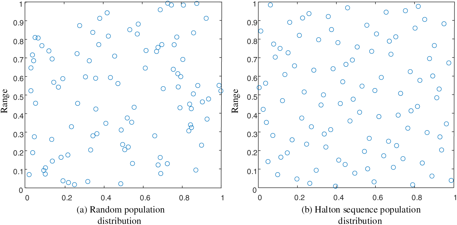
Figure 1: Initial population distribution

As can be seen from Fig. 1, Halton’s pseudo-random sequence of populations has some randomness and a more even distribution of populations, and there are no very close and overlapping individuals with small search blindness. Using this pseudo-random sequence to initialise the population effectively improves the diversity of the initialisation, produces a higher quality of candidate solutions and avoids the chance of the algorithm due to random initialisation. Its mapping to the population space is as follows:

xid=H(n)⋅(ubd−lbd)+lbd(18)

where xid denotes the Halton sequence initialised particle population, ubd and lbd are the upper and lower boundaries of the d dimensional space respectively.

3.2.2 Introduction of Adaptive T-Distribution Perturbations

For any intelligent algorithm, both local search capability and global search capability are indispensable. The traditional PSO algorithm particle population has convergent characteristics and has a strong local search capability. However, the weak ability of the individual particle population to explore the unknown space leads to its poor global convergence ability. In general, the way to enhance the global search capability lies in increasing the population diversity and avoiding population aggregation. Therefore, in order to further enhance the population diversity in the late iteration and improve the global search capability of the algorithm, this paper adds adaptive t-distribution variation to the process of population particle position updating.

The Cauchy variational operator and the Gaussian variational operator are commonly used variational operators to improve the performance of intelligent optimization algorithms. The standard Gaussian distribution density N(0,1) has an expectation of 0 and a variance of 1. The standard Cauchy distribution probability density C(0,1) has no expectation and an infinite variance. The standard Gaussian distribution and the variance of the Corsi distribution are very different, and the performance shows that the Gaussian variance operator has a stronger search ability in local exploitation and can improve the convergence speed to some extent, while the Corsi variance operator has a stronger ability in global search and can maintain the diversity of the population during the iteration. The adaptive t-distribution variant combines the advantages of both and treats the number of iterations n as a degree of freedom parameter, whose expression and probability density function are:

t=XY/n,X∼N(0,1),Y∼x2(n)(19)

p(x)=Gam((n+1)/2)nπGam(n/2)(1+x2/n)−(n+1)/2,x∈(−∞,∞)(20)

when n=1, the t distribution can be transformed into the standard Kersey distribution, while as n tends to infinity, the t distribution is gradually transformed into the standard Gaussian distribution. The standard Kersey distribution and the Gaussian distribution are the two boundary special case distributions of the t distribution. The distribution function is shown in Fig. 2.

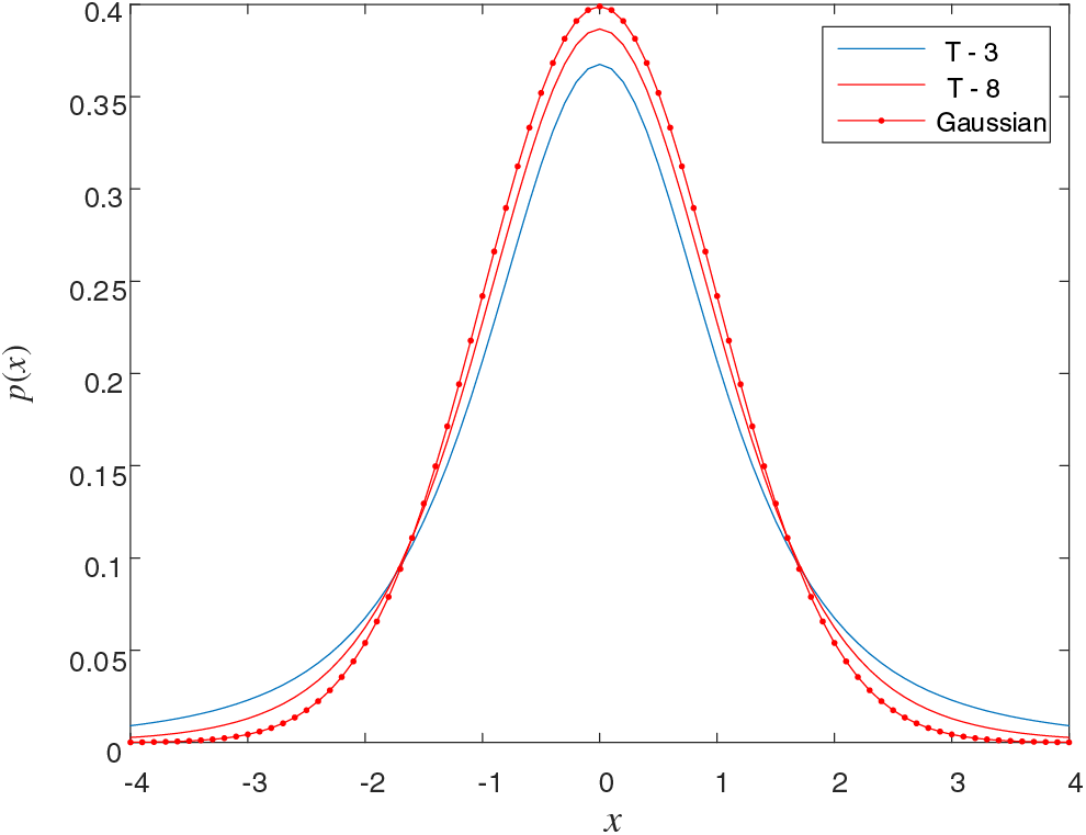
Figure 2: Distribution function probability density curve

Using the adaptive t-distribution perturbation to optimise the particle swarm algorithm, the adaptive t-distribution perturbation is introduced into the process of particle position updating to achieve a population variation process as in Eq. (21).

xit=xi+xi⋅t(iter)(21)

where xit is the position of the individual after the variation of the t-distribution; t(iter) is the t-distribution with the number of iterations of the algorithm as the degrees of freedom. Taking the number of iterations as the degrees of freedom of the t-distribution, as the number of iterations increases, the curve change is characterized by first conforming to the Coasean distribution and later approaching the Gaussian distribution. This process is also exactly adapted to the variation state of the algorithm search process, using the t-distribution for optimal position variation, improving the efficiency of the algorithm variation to enhance the convergence accuracy.

3.3 Algorithm Flow

For the optimal configuration model of measurement points established in this paper, the objective function 1 is expressed uniformly in combination with the constraints of Eqs. (6) and (8) to define the fitness function value F(h):

minF(h)=f1(h)+δe(h)(22)

e(h)=min(0,∑i=1nh(i)⋅A(i,j)−1)2+min(0,‖h‖1−Kln⁡NK)2(23)

where δ is the penalty factor and takes a large enough positive value.

An improved particle swarm optimisation algorithm is applied to solve the measurement point optimisation configuration model, the algorithmic flow of which is shown in Fig. 3.

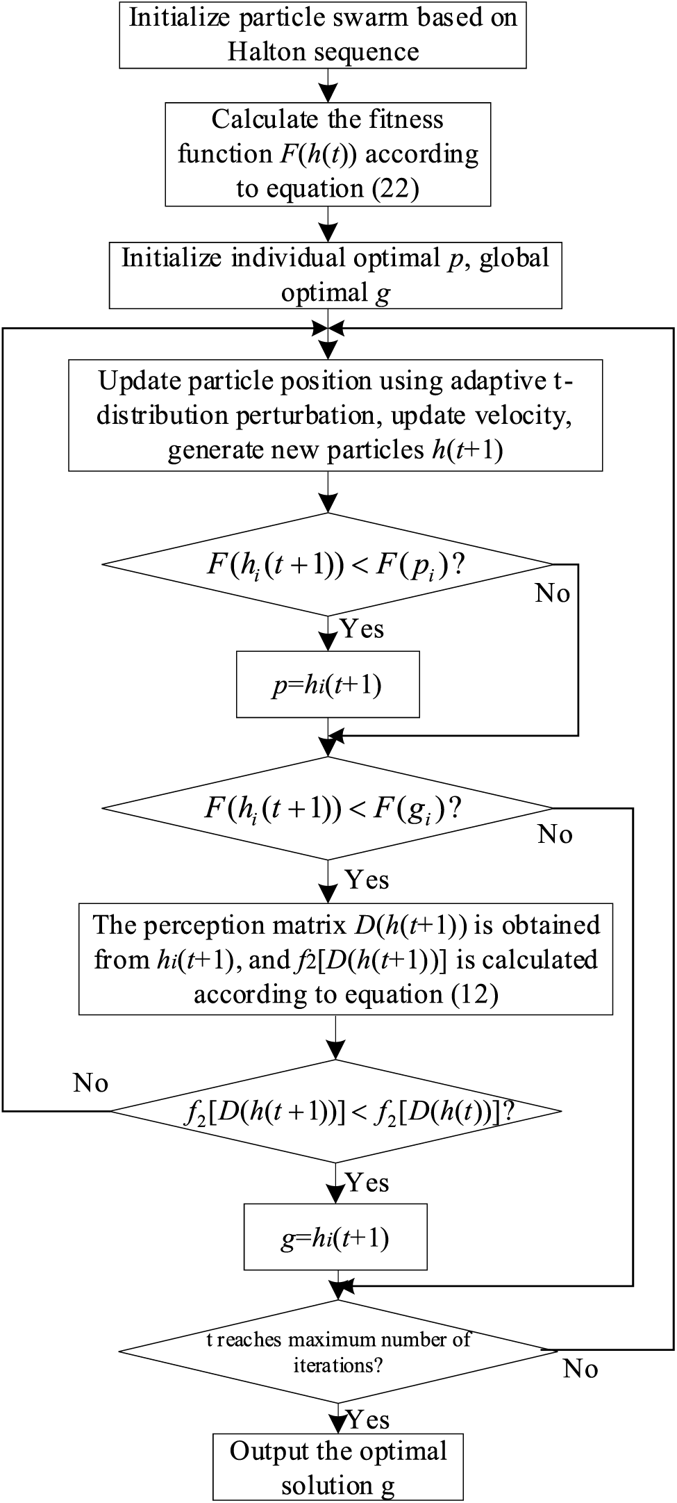
Figure 3: Flow chart of the optimization algorithm

1.    The Halton pseudo-random sequence is introduced to initialise the initial position of the population, setting the number of particles, their dimensions and the maximum number of iterations.

2.    Calculate the initial fitness value of the individual particle according to Eq. (22).

3.    The initial fitness value is used as the current pre-historic optimal solution for each particle, and the population best initial fitness value is used as the current global optimal solution.

4.    The velocity of each particle is updated and the particle position is updated according to Eq. (21) by introducing an adaptive t-distribution perturbation strategy.

5.    Compare whether the current fitness value of each particle is better than the historical individual optimum, if so, the current particle fitness value is taken as the individual optimum of the particle and its corresponding position is taken as the position where the individual optimum of each particle is located.

6.    Compare the historical optimum of the whole population and calculate whether the average number of interrelationships of the perception matrix obtained from the current optimum is lower than that obtained from the historical optimum according to Eq. (12), and if it is lower, then it is taken as the historical optimum of the whole population, i.e., the global optimum solution.

7.    Repeat steps (4) to (6) until the set maximum number of iterations is met.

8.    The global optimal solution of the output particle swarm is the optimised measurement point configuration.

4  Experimental and Simulation Analysis

4.1 Performance Analysis of Improved Particle Swarm Optimization Algorithms

Based on the MATLAB R2020a simulation platform, the effectiveness of the improved particle swarm optimization algorithm and the reliability of the algorithm solution operation are verified, and the original classical particle swarm algorithm and the adaptive weight particle swarm algorithm are introduced for simulation comparison and analysis. In the improved particle swarm optimisation algorithm, the number of population particles set is 20, the learning factor c1=c2=2.0, the maximum number of iterations is T=100, the maximum velocity v=2 and the inertia weight decreases linearly from 0.9 to 0.4 in the iterations.

Six test functions from the reference [21] are selected as benchmark test functions for function optimisation testing, as shown in Fig. 4, which contain single-peak functions with only one optimal value for verifying the convergence performance of the algorithms; multi-peak functions with multiple local optimal solutions for verifying the ability of the algorithms to jump out of the local optimums; and composite functions for verifying the comprehensive performance of the algorithms. A comparison of the evolutionary process curves of the improved particle swarm algorithm with the classical particle swarm algorithm, the adaptive weighted particle swarm algorithm, the genetic algorithm, and the ant colony algorithm for the six test functions is shown in Fig. 5. The superiority of the improved algorithm in this paper is reflected by comparing it with other modern methods.

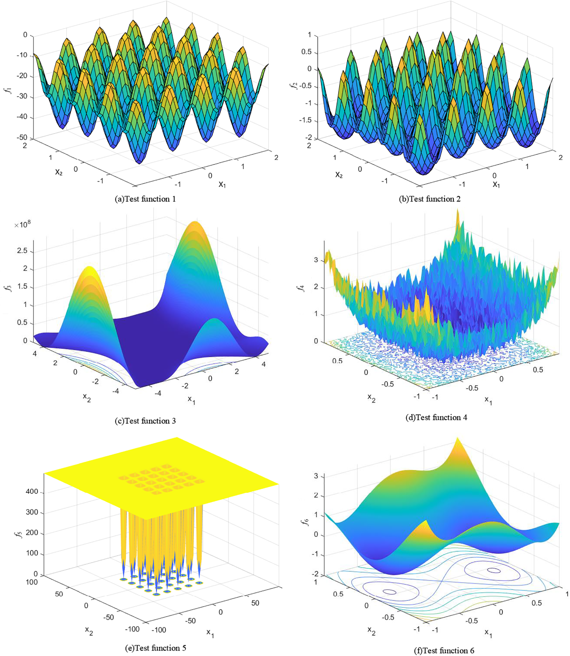
Figure 4: 6 test functions

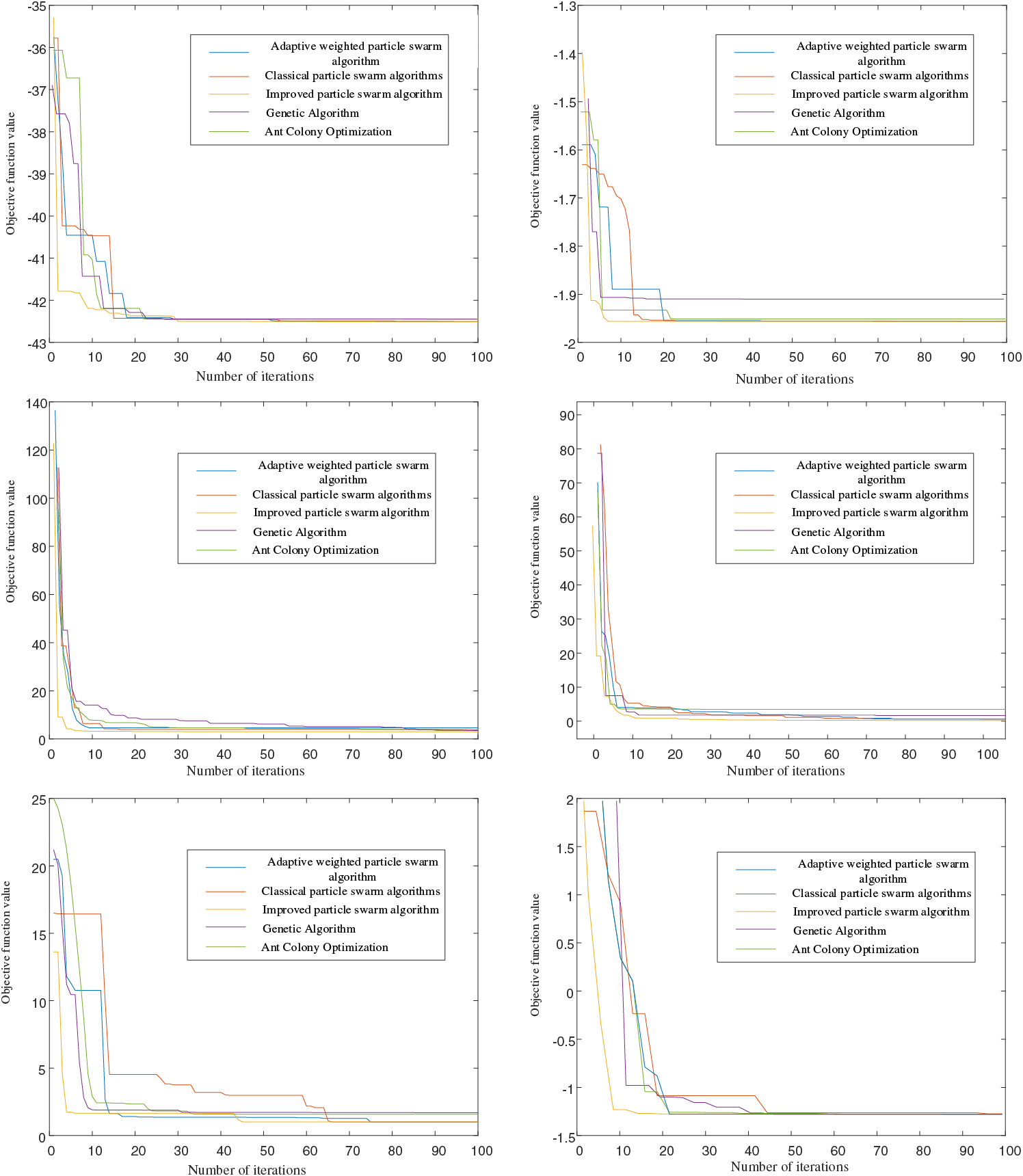
Figure 5: Comparison of convergence plots for the six tested functions

The convergence curve of the test function is plotted for observation, which can more intuitively see the convergence speed of the algorithm and how fast it changes. The convergence curve of the optimization algorithm in different functions is verified to compare its convergence fast and slow change trend. If the convergence speed is faster, it shows that the algorithm converges better results, the higher the efficiency of the optimization search, and the fast convergence ability of the algorithm can be judged from the convergence curve, which is also sufficient to illustrate the advanced nature of the algorithm. The convergence curves of the six functions in Fig. 5 show that the improved particle swarm optimisation algorithm has the best convergence effect. The introduction of adaptive t-distribution is more adaptable to the search of the algorithm and enables the algorithm to reach the optimal value quickly. The introduction of the Halton sequence to initialise the population has a clear trend of convergence at the beginning of the iteration, indicating that it can better initialise the population evenly, which can quickly find the local range of the target location and improve the search efficiency of the algorithm. Overall, the improved algorithm has greater local search capability and global search capability.

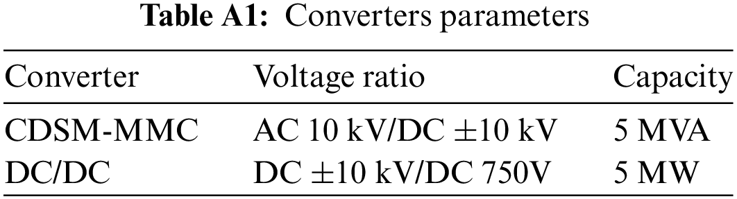
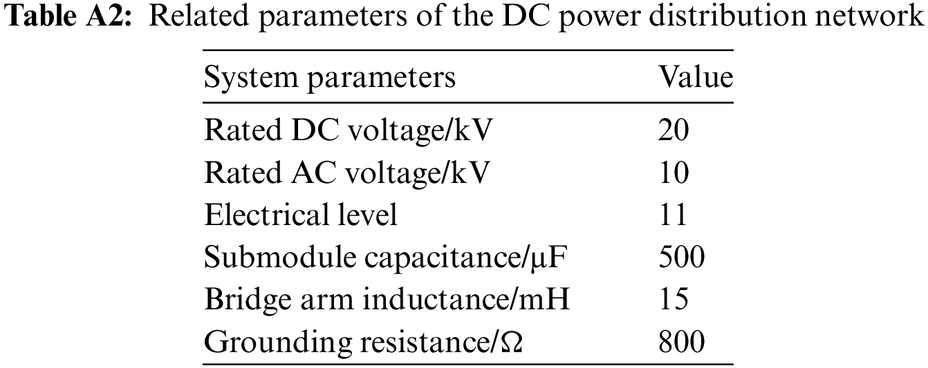
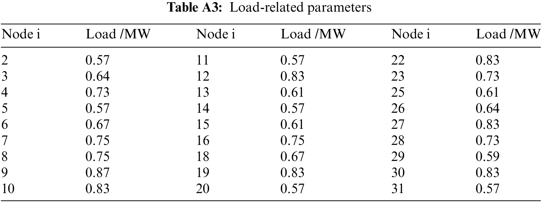
4.2 Perform Simulation for Optimal Configuration of Measurement Points

The simulation algorithm in this paper is built based on the PSCAD/EMTDC platform, and based on the structure and parameters of the original IEEE33 node distribution network, the DC distribution network is built, with a system voltage level of ±10 kV, using the neutral non-effective grounding method, including 31 branch circuits, five nodes accessed by AC system via MMC, and DC loads are accessed at some of the nodes at the same time, and so on. As shown in Fig. 6, the black circle indicates the common DC load node, the red circle indicates the node of AC system accessed via MMC, and the red box indicates the selected location of the measurement point. The specific parameters and loads of the line are shown in Appendix Tables A1–A3. In order to demonstrate the rationality of the proposed method in this paper, the proposed fault location measurement point optimisation configuration method is used to simulate the configuration of the measurement points of the constructed DC distribution network. The improved particle swarm algorithm is set with an initial population of 40, a learning factor of c1 = c2 = 1.8, a maximum number of iterations of 100 and inertia weights that decrease linearly from 0.95 to 0.4. Fig. 7 shows the iterative convergence curve of the improved particle swarm algorithm and other modern optimization algorithms in the process of optimizing the measurement points, which reaches convergence in about 12 iterations, and the improved particle swarm algorithm converges faster, and the number of optimized measurement points is obtained as 6. Fig. 8 shows the final results of the measurement point locations after optimisation, and the six measurement points correspond to nodes 8, 18, 21, 22, 26 and 31 of the 32-node DC distribution network. The structure of the DC distribution network and the installation location of the optimised measurement device are shown in Fig. 6.

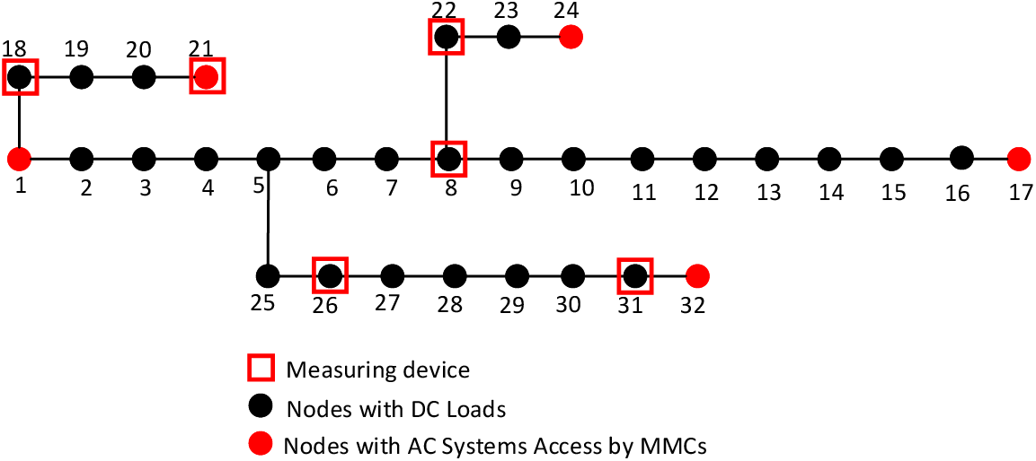
Figure 6: 32-node DC distribution network and measurement point installation locations

Figure 7: Iterative convergence curve

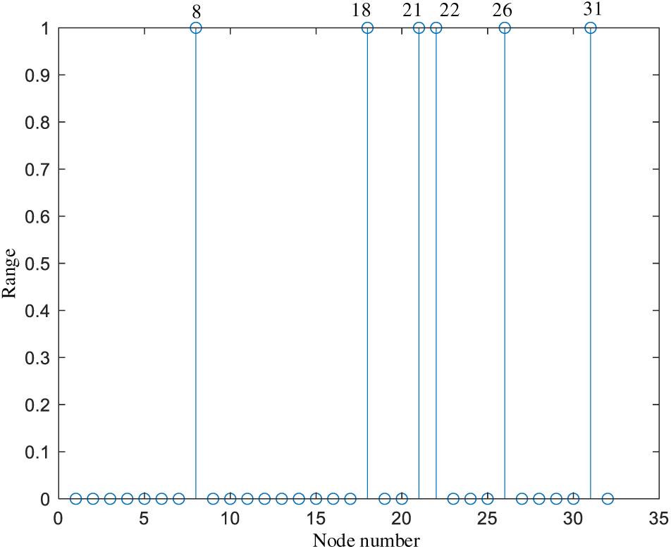
Figure 8: Optimised measurement points

4.3 Fault Location Simulation Validation of New Configuration Solutions

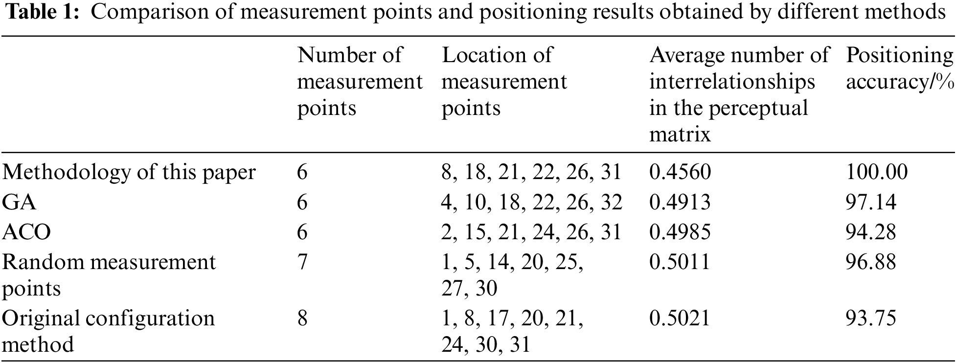
In order to verify the accuracy of the optimised configuration of DC distribution network fault location measurement points based on the improved particle swarm optimisation algorithm proposed in this paper, 55 bipolar short circuit faults were randomly selected from the 31 branches of the above DC distribution network for multiple fault location simulation experiments. The positioning results of the measurement points obtained by this paper’s method are compared and analysed with those obtained by other methods. As shown in Table 1, the average number of interrelationships of the perceptual matrices constructed by the six measurement points obtained after the optimisation of this paper’s method is lower than the average number of interrelationships of the perceptual matrices constructed by the configurations of the measurement points obtained by the other methods, which can indicate that the sparse current vectors can be reconstructed better during the process of compressed perceptual reconstruction, and that the accuracy of fault location of the measurement points obtained by this paper’s method is the highest.

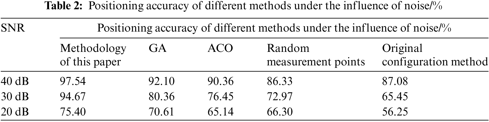
Because there are important components in the DC distribution network such as converter composed of power electronic devices, its structure is complex, and it will produce a certain amount of noise when the system is running, which is one of the important factors affecting fault location. Therefore, we use Gaussian white noise to simulate the noise when the system is running and carry out simulation experiments. Signal-to-noise ratio (SNR) of 40, 30, 20 dB, the fault location results are compared as shown in Table 2. It can be seen that the measurement point configuration scheme selected in this paper still has a high fault location accuracy compared with other measurement point configuration schemes under the influence of noise. It shows that the measurement points obtained from this paper have good resistance to certain noise, but when the signal-to-noise ratio reaches 20 dB, the noise has a greater impact on the positioning results, and the positioning error caused at this time is difficult to avoid.

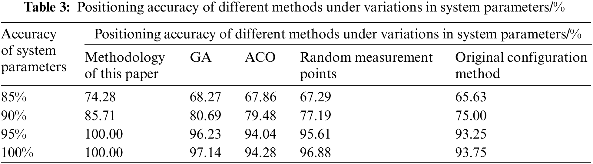
Since the compressed sensing theory utilised in this paper for fault location is directly related to the accuracy of the node impedance matrix elements, for this reason the accuracy of the DC distribution system parameters is set to be 85%, 90%, 95% and 100%, respectively. Comparison of the location accuracy of the measurement point configuration scheme obtained by the methodology of this paper under the uncertainty of the system parameters with the configuration scheme obtained by the other methods is shown in Table 3. From the table, it can be seen that the fault location accuracy of the configuration scheme obtained from the method of this paper does not change much from the other configuration schemes when the error is within 5%. A parameter error of 10% or more leads to a large change in the elements of the node impedance matrix, while this paper’s method takes into account the perceptual matrix, i.e., the average number of interrelationships of the node impedance matrices during the optimisation process of the measurement point configurations, which improves the reconstruction effect compared to the other schemes when reconstructing the sparse fault currents, and therefore the localisation accuracy of this paper’s configurations is improved under the uncertainty of the system parameters.

5  Conclusion

This paper applies the improved PSO algorithm to achieve an accurate and optimal configuration of fault location measurement points in DC distribution networks, satisfying the requirement of network-wide observability by reasonably setting the minimum number of measurement device locations, and combining the influence of the construction of the perception matrix on the reconstruction effect in compressed sensing theory to improve the location accuracy. An economic and reasonable system model for the optimal allocation of measurement points is initially constructed. Compared with the traditional point optimization theory, it overcomes the disadvantages of large computation and blind location selection, improves the positioning accuracy, and makes the solution more accurate and fast with the improved PSO algorithm. Through a large amount of simulation data, this paper shows that the optimal configuration of fault location measurement points in DC distribution network based on improved particle swarm optimization algorithm greatly reduces the cost of monitoring network, improves the monitoring efficiency, provides good technical support for further prevention and management of distribution network fault problems, and has important engineering application value.

Acknowledgement: None.

Funding Statement: This work was supported by the National Natural Science Foundation of China (52177074).

Author Contributions: The authors confirm contribution to the paper as follows: study conception and design: Huanan Yu, Hangyu Li; data collection: He Wang; analysis and interpretation of results: Shiqiang Li, Hangyu Li, Huanan Yu. Author; draft manuscript preparation: Hangyu Li, Shiqiang Li. All authors reviewed the results and approved the final version of the manuscript.

Availability of Data and Materials: The authors confirm that the data supporting the findings of this study are available within the article and/or its supplementary materials.

Conflicts of Interest: The authors declare that they have no conflicts of interest to report regarding the present study.

References

1. Liu, H., Deng, Z. F., Li, X. L., Guo, L., Huang, D. et al. (2022). The averaged-value model of a flexible power electronics based substation in hybrid AC/DC distribution systems. CSEE Journal of Power and Energy Systems, 8(2), 452–464. [Google Scholar]

2. Li, Z., Duan, J., Lu, W., Du, X., Yang, W. et al. (2021). Non-permanent pole-to-pole fault restoration strategy for flexible DC distribution network. Journal of Modern Power Systems and Clean Energy, 9(6), 1339–1351. https://doi.org/10.35833/MPCE.2021.000240 [Google Scholar] [CrossRef]

3. Wei, Y. F., Wang, Z. J., Wang, P., Zeng, Z. H., Wang, X. W. (2022). Protection method for flexible DC distribution network faults based on current limiting reactance voltage. High Voltage Engineering, 48(12), 5068–5079. [Google Scholar]

4. Li, Y., He, L., Liu, F., Li, C., Cao, Y. et al. (2019). Flexible voltage control strategy considering distributed energy storages for DC distribution network. IEEE Transactions on Smart Grid, 10(1), 163–172. https://doi.org/10.1109/TSG.2017.2734166 [Google Scholar] [CrossRef]

5. Lu, F. Y., Chen, Z. X., Feng, Y. F., Mang, Z. (2022). Line protection method of DC distribution network based on high and low frequency voltage amplitude ratio. Automation & Instrumentation, 37(12), 6–11. [Google Scholar]

6. Mei, J., Zhang, B. T., Zhu, P. F., Ge, R., Yan, L. X. (2021). Fault location method of flexible DC distribution network based on active control of fault current. Automation of Electric Power Systems, 45(24), 133–141. [Google Scholar]

7. Zhong, Q., Feng, J. J., Wang, G., Li, H. F. (2019). Analysis of resonance characteristics of DC distribution network based on node impedance matrix. Proceedings of the CSEE, 39(5), 1323–1334 (In Chinese). [Google Scholar]

8. Liu, Y. W. (2012). Active protection and control technique based on smart high voltage equipment. Power System Technology, 36(12), 71–75. [Google Scholar]

9. Tang, Z., Liu, J. Y., Liu, Y. B., Li, T., Xu, W. T. (2018). Load control and distribution network reconfiguration with participation of air-conditioning load aggregators. Automation of Electric Power Systems, 42(2), 1−10+49. [Google Scholar]

10. Li, D. M., Hu, Y. Y., Wang, L. L., Li, M. G., Li, X. S. (2019). Double-end distance measurement fault location method for DC distribution network based on improved injection method. Smart Power, 47(12), 110–116. [Google Scholar]

11. Han, J. H., Zhang, M., Luo, G. M., Yu, B., Hong, Z. Q. (2017). A fault location method for flexible DC distribution network based on fault transient process. Power System Technology, 41(3), 985–992. [Google Scholar]

12. Li, M., Ja, K., Bi, T. S., Yang, G. S., Liu, Y. et al. (2016). Fault distance estimation-based protection for DC distribution networks. Power System Technology, 40(3), 719–724. [Google Scholar]

13. Song, G. B., Wang, T., Zhang, C. H., Wu, L. (2019). Adaptive auto-reclosing of DC line based on characteristic signal injection with FB-MMC. Power System Technology, 43(1), 149–156. [Google Scholar]

14. Song, G. B., Wang, T., Zhang, C. H., Wu, L. (2019). DC line fault identification based on characteristic signal injection using the MMC of sound pole. Transactions of China Electrotechnical Society, 34(5), 994–1003. [Google Scholar]

15. Yang, L. H., Yang, M. Y. (2013). The design of transmission and transformation equipment anti-accident measure dynamic management information system based on ASP.NET and SQL. Electric Power Science and Engineering, 29(6), 12–16. [Google Scholar]

16. Song, G. B., Hou, J. M., Guo, B. (2021). Single-ended fault location of hybrid MMC-HVDC system based on active detection. Power System Technology, 42(5), 730–740. [Google Scholar]

17. Rozenberg, I., Beck, Y., Eldar, Y. C. (2018). Sparse estimation of faults by compressed sensing with structural constraints. IEEE Transactions on Power Systems, 33(6), 5935–5944. https://doi.org/10.1109/TPWRS.2018.2823734 [Google Scholar] [CrossRef]

18. Jia, K., Yang, B., Dong, X. Y., Feng, T., Bi, T. S. (2020). Sparse voltage measurement-based fault location using intelligent electronic devices. IEEE Transactions on Smart Grid, 11(1), 48–60. https://doi.org/10.1109/TSG.2019.2916819 [Google Scholar] [CrossRef]

19. Jia, K., Dong, X. Y., Li, L., Feng, T., Bi, T. S. (2020). Fault location for distribution network based on transient sparse voltage amplitude measurement. Power System Technology, 44(3), 835–845. [Google Scholar]

20. Jia, K., Feng, T., Zhao, Q. J., Wang, C. B., Bi, T. S. (2020). Bipolar short-circuit fault location for DC distribution network based on sparse measurement of fault high-frequency voltage. Automation of Electric Power Systems, 44(1), 142–151. [Google Scholar]

21. Cui, J., Li, S., Yu, J. W. (2021). Optimal PMU placement method based on improved grey wolf optimizer. Information Technology, 21(8), 75–80. [Google Scholar]

22. Zhao, Y. Y., Yuan, P., Ai, Q., Lu, T. G. (2014). Improved genetic algorithm based optimal configuration of PMUs considering topological constraints. Power System Technology, 38(8), 2063–2070. [Google Scholar]

23. Liu, Y. P., Li, X., Zeng, S. Q., Wu, J. K., Zhang, H. Y. et al. (2021). PMU optimal configuration of distribution system for interval state estimation. Southern Power System Technology, 15(7), 67–75. [Google Scholar]

Appendix