 Open Access
ARTICLE
Data-Driven Modeling for Wind Turbine Blade Loads Based on Deep Neural Network
1 Yangjiang Power Supply Bureau, Guangdong Power Grid, Yangjiang, 529500, China
2 Energy and Electricity Research Center, Jinan University, Zhuhai, 519070, China
* Corresponding Author: Qi Yao. Email:
(This article belongs to the Special Issue: AI-application in Wind Energy Development and Utilization)
Energy Engineering 2024, 121(12), 3825-3841. https://doi.org/10.32604/ee.2024.055250
Received 21 June 2024; Accepted 21 August 2024; Issue published 22 November 2024
Abstract
Blades are essential components of wind turbines. Reducing their fatigue loads during operation helps to extend their lifespan, but it is difficult to quickly and accurately calculate the fatigue loads of blades. To solve this problem, this paper innovatively designs a data-driven blade load modeling method based on a deep learning framework through mechanism analysis, feature selection, and model construction. In the mechanism analysis part, the generation mechanism of blade loads and the load theoretical calculation method based on material damage theory are analyzed, and four measurable operating state parameters related to blade loads are screened; in the feature extraction part, 15 characteristic indicators of each screened parameter are extracted in the time and frequency domain, and feature selection is completed through correlation analysis with blade loads to determine the input parameters of data-driven modeling; in the model construction part, a deep neural network based on feedforward and feedback propagation is designed to construct the nonlinear coupling relationship between the unit operating parameter characteristics and blade loads. The results show that the proposed method mines the wind turbine operating state characteristics highly correlated with the blade load, such as the standard deviation of wind speed. The model built using these characteristics has reasonable calculation and fitting capabilities for the blade load and shows a better fitting level for untrained out-of-sample data than the traditional scheme. Based on the mean absolute percentage error calculation, the modeling accuracy of the two blade loads can reach more than 90% and 80%, respectively, providing a good foundation for the subsequent optimization control to suppress the blade load.Keywords
Nomenclature
| Mf | Flapwise bending moment |
| Me | Edgewise bending moment |
| Vrel | Relative wind speed |
| V0 | Wind speed |
| r0 | Hub radius |
| l | Chord length |
| Cl | Lift coefficient |
| Cd | Drag coefficient |
| α | Attack angle |
| β | Pitch angle |
| I | Inflow angle |
| a | Axial induction factor |
| b | Tangential induction factor |
| σ | Stress amplitude |
| N | Number of stress cycles experienced by the material |
| C | Maximum force on the material |
| m | Wöhler coefficient |
| nj | Number of cycles at stress level σj |
| Nj | Number of cycles at which the stress σj causes the component to fail |
| Ns | Number of sampling points in the calculation period |
| x(i) | Wind turbine operating condition sampling point i |
| Np | Number of sampling points in the calculation period |
| u(n) | Sampled data converted into frequency domain signal |
| ωr | Rotor speed |
| Ti | Turbulence intensity |
| Pe | Active power |
| Abbreviation | |
| C1 | Comparison scheme 1 |
| C2 | Comparison scheme 2 |
| CMS | Central monitoring system |
| DEL | Damage equivalent load |
| DNN | Deep neural network |
| ELU | Exponential linear unit |
| MAPE | Mean absolute percentage error |
| NREL | National renewable energy laboratory |
| OpenFAST | Open fatigue, aerodynamics, structures, turbulence interface |
| P-DNN | Proposed DNN model |
| ReLU | Rectified linear unit |
| RMSE | Root mean square error |
| SCADA | Supervisory control and data acquisition |
| SeLU | Scaled exponential linear unit |
| TCV | Theoretical calculation value |
As an essential component of energy capture, the blades of wind turbines are both essential and relatively fragile. Optimizing and controlling fatigue damage during operation can help extend their service life [1,2]. One of the most critical tasks is to define fatigue damage accurately.
There are many methods to define fatigue damage of wind turbine blades, each with its advantages and disadvantages. The most intuitive method is to define it based on expert experience. In [3], researchers believe that the structural damage of wind turbines is a custom function relationship related to power generation and wind field turbulence. Similar indicators are common in the optimal control of wind farms [4,5]. In addition to the custom function model, some literature defines fatigue damage based on the standard deviation of fatigue stress. For example, reseaechers [6–8] focused on the blade bending moment and used its fluctuation as an indicator to measure blade damage. However, whether it is the custom damage function or the stress standard deviation method, the relevant indicators can only partially linearly represent the fatigue load. As described in [9], stress and corresponding fatigue load are generated. However, the torque generated by the mechanical structure may be the same under different environments and conditions, so fatigue damage can not be represented by torque [10].
In contrast, fatigue assessment methods that use rain flow counting [11] and the Palmgren-Miner method [12] to represent load changes and calculate DEL [13] are more accurate and have been widely recognized by researchers in practical applications and simulations [14,15]. However, the principle of DEL is complex and difficult to calculate, so it is generally only used to evaluate fatigue loads in wind farms. It can not be applied to real-time power control.
In order to introduce accurate load indicators in real-time control or scheduling, data-driven load modeling methods have received attention in recent years [16]. Some researchers use relatively simple fitting or regression methods such as static lookup table method [17], arbitrary polynomial chaos expansion [18], or support vector machine [19] to model loads, but such methods usually lack good generalization ability and the accuracy of modeling data outside the training sample is not guaranteed. Furthermore, some more complex methods have been introduced into the modeling process, such as neural networks [20,21], DNN [22], and deep residual recurrent neural networks [23]. More complex network structures help better describe the nonlinear coupling relationship. However, the relevant literature needs standardized design schemes for the inputs required for modeling, which are usually only subjective settings based on human experience. As for the data source required for modeling input, most studies choose to use wind farm SCADA system data, as introduced in [20–23]. A small number of studies require the installation of additional sensors [24] or the use of CMS data [25]. For wind farms, additional sensors or CMS systems will increase costs, so it is more feasible only to use SCADA system data.
Given the above research status and shortcomings, this project intends to conduct data-driven modeling for the DEL indicators of wind turbine blades. The specific innovations are:
• A DEL calculation model for wind turbine blades based on a DNN framework is proposed;
• By mechanism analysis, this paper ensures that the model input is only the easily measurable data of the SCADA system;
• A feature extraction method is designed based on correlation analysis, which can standardize the design of the DNN input and improve the generalization ability.
The following sections are arranged as follows: Section 2 summarizes the overall architecture of the methodology; Section 3 analyzes the parameters required for blade load data-driven modeling based on the generation mechanism and theoretical calculation method of blade load; Section 4 proposes a feature extraction and deep learning method to construct a DEL calculation model; Section 5 uses OpenFAST for simulation verification and discussion; Section 6 is the conclusion.
2 Overall Architecture of Methodology
This paper aims to perform data-driven modeling of wind turbine blade fatigue loads to avoid overly complex theoretical calculations. The methods to be used in this paper include 1) theoretical analysis of the calculation method of wind turbine blade loads, screening of easily measurable operating parameters related to wind turbine blade loads; 2) feature selection of the screened operating parameter time series data, extracting feature sets to construct data-driven model inputs; 3) using a deep neural network model to construct a coupling model between feature sets and blade loads, and realizing rapid calculation of blade loads. The overall methodology architecture is shown in Fig. 1, and the following two sections will explain the specific implementation of each step.
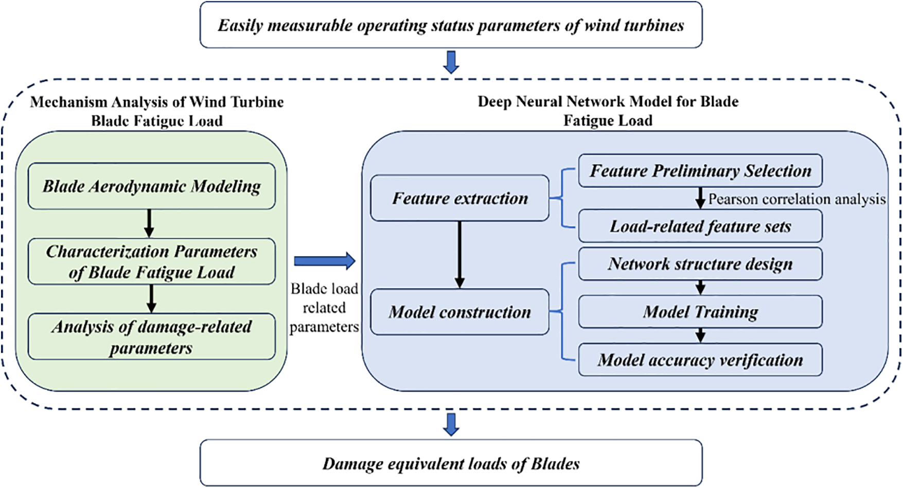
Figure 1: The methodological framework of this study
3 Mechanism Analysis of Wind Turbine Blade Fatigue Load
This section will introduce the mechanism model and theoretical calculation method of blade fatigue load and, based on this, explore the easily measurable operating parameters associated with blade fatigue load as the theoretical basis for data-driven modeling.
3.1 Blade Aerodynamic Modeling
Fig. 2 shows the element analysis of a blade based on the blade element momentum theory. The blade structure is like a cantilever beam, so the moment at its root can be regarded as the primary source of structural damage. Mf and Me of the blade root can be expressed as [26]:
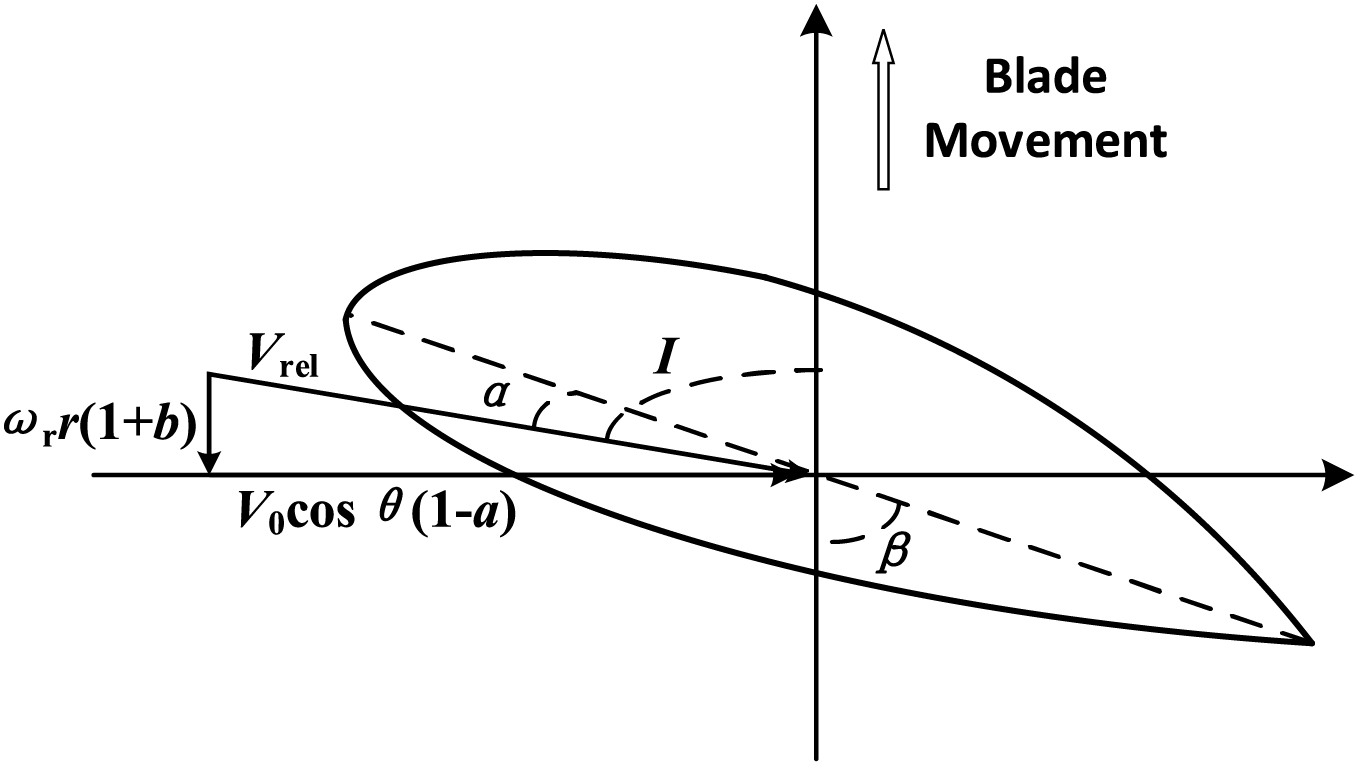
Figure 2: Analysis of blade element
When the yaw deviation angle θ does not equal 0, the relative wind speed can be expressed as:
3.2 Characterization Parameters of Blade Fatigue Load
Based on Mf and Me, the DEL of the blade in two directions can be further calculated to more accurately characterize the fatigue characteristics of the blade. By definition, DEL is the amplitude of the sinusoidal stress at a constant frequency f over time T that produces the same damage as the original stress signal. Using the Palmgren-Miner rule [27] and the S-N curve [28], the calculation method of DEL [29] can be determined as follows:
In this paper, the calculation of DEL uses the MCrunch code [13], which can be calculated in MATLAB. However, the calculation of DEL requires the use of measurement data of the two torque parameters, Mf and Me, over a period of time. This requires additional sensors to measure these two torques and continuously record a large amount of data over a specific period, which is not easy to achieve.
3.3 Analysis of Damage-Related Parameters
The DEL calculation of the blade is based on the two moments of blades, Mf and Me. According to Eqs. (1)–(3), Mf and Me of the wind turbine blade are related to multiple variables such as relative wind speed, attack angle, lift coefficient, drag coefficient, and pitch angle. Among them, the lift and drag coefficient can also be described as related functions with the attack angle as a variable. According to Eq. (4), the relative wind speed is related to actual V0 and ωr. The attack angle is the angle between the blade chord and relative wind speed, which is related to its operating conditions and can be a function of the Pe.
In summary, the subsequent sections will select the measured V0, β, ωr, and Pe as input parameters to establish a blade fatigue load model driven by measurable data.
4 Deep Neural Network Model for Blade Fatigue Load
In this section, based on the selected wind turbine operating state parameters, a feature set related to blade loads will be constructed as modeling input. Then, a deep neural network will be designed to realize data-driven blade load modeling.
According to the above analysis, four parameters are selected as the input parameters of the data-driven model. However, these wind turbine operating parameters are recorded as time series. The amount of data is significant, and it is not easy to use all of them directly as input. Therefore, this section will extract features from multiple time series and filter them based on correlation as direct input to the neural network model. For the above time series signals, effective features can usually be extracted from the time and frequency domain [30].
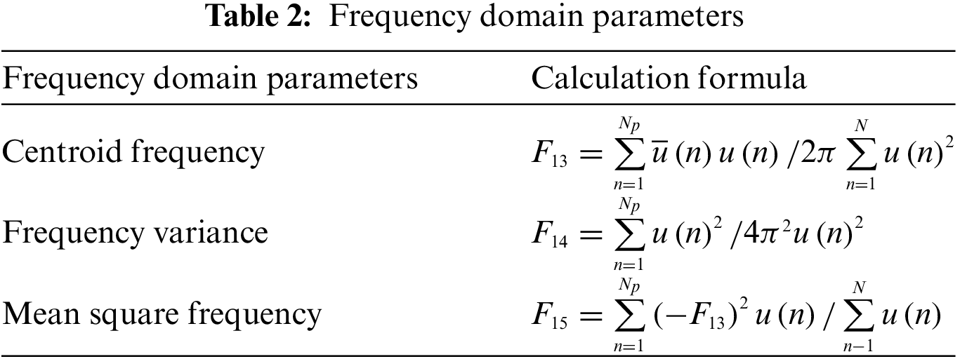
The time domain analysis method obtains the dynamic change law by describing the autocorrelation structure of the time series. This method is relatively simple and easy to understand. The frequency domain analysis method is most commonly used in Fourier transform analysis and wavelet analysis, which are used to quantify the periodicity or the multi-scale time pattern characteristics [31]. The time and frequency domain parameters are exhibited in Tables 1 and 2.

In Table 1, there are 12 sets of characteristic parameters for the time domain, among which the peak value is also called the maximum value, and the peak difference is the difference between the peak and minimum. When a wind turbine usually operates, the peak and minimum values will not fluctuate too much. If there is a significant deviation from the normal value, it can be judged that the wind turbine has a fault. The abnormal maximum and minimum values and peak differences can also screen normal data. The average value and the rectified average value reflect the average parameters of the data of each working condition when the wind turbine is running, which can represent the changing relationship between different working conditions. The variance, standard deviation, and root mean square values can represent the degree of fluctuation of the working condition within the sampling time. Kurtosis and margin factors are more sensitive to impact signals and can characterize whether the working condition has a change within the sampling time. Skewness is used to measure the asymmetry of the time series, that is, the degree of deviation between the more extensive working condition and the more minor working condition relative to the average value.
In Table 2, the centroid frequency is the frequency of the more significant component in the spectrum, describing the distribution of the power spectrum. The frequency variance is the square of the frequency standard deviation, which can quantify the degree of spectral energy dispersion. The mean square frequency is the weighted average of the square of the root mean square frequency.
In the calculation process of the characteristic parameters mentioned above, the calculation period is 5 min, and the sampling interval is 1 s.
Tables 1 and 2 show that some commonly used time domain and frequency domain indicators are included. These indicators can universally analyze the characteristics of time series data, but not all are related to the DEL to be calculated. Therefore, before being used for DEL modeling, an analysis based on Pearson correlation will be performed first. Indicators with correlation coefficients higher than 0.6 can be considered solid correlation parameters [32] and will be screened as the input of the corresponding DEL model in the subsequent modeling process. The formula of the Pearson correlation coefficient is [32]:
The prototype of a deep neural network is a discriminant model. Knowing the input variable can infer the value of the output variable. Generally speaking, the internal network structure of a DNN is shown in Fig. 3.
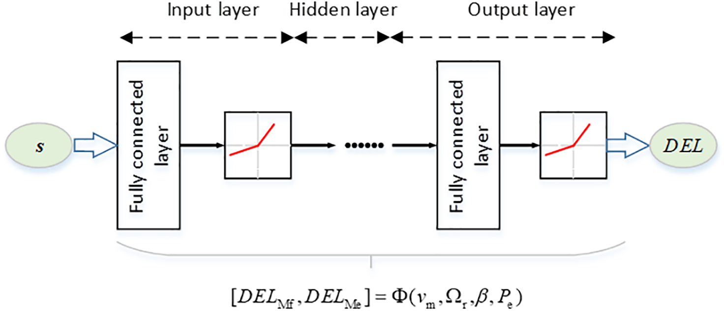
Figure 3: Deep neural network structure diagram
Unlike traditional perceptrons, the deep neural network also contains backpropagation and forward channels. The back-propagation channel compares the outputs with the true values and propagates the calculated error back to the input layer by layer. In the subsequent process, the parameters in the forward propagation process are adjusted to minimize the impact of the error value on the network. The idea of model construction can be found in our previous work [22]. After determining the structure of the DNN, the network training process is shown in Algorithm 1.
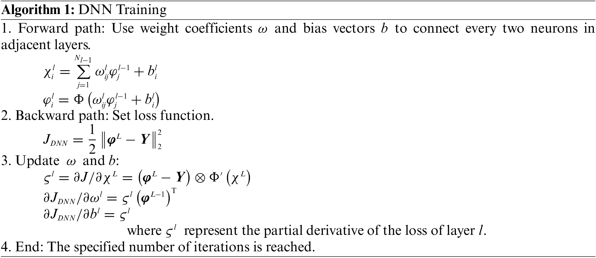
During forward propagation modeling, an activation function is generally required to introduce nonlinear factors in the propagation process in addition to the linear relationship. Commonly used activation functions in deep neural networks include Sigmoid, ReLU, Leaky ReLU, etc. In the experiment, it is necessary to screen the activation function with the best effect through multiple parameter settings.
During backpropagation modeling, a reasonable loss function is critical, which can be used to measure the deviation between the output calculated by the training data and the true output, and update ω and b based on iteration and forward propagation. Common loss functions include mean square error, etc.
ω and b can be updated as Algorithm 1. However, in the training process, as the depth of the DNN increases, the parameters can be gradually deviate from their set range during the update process. To address this problem, this paper uses the Adam algorithm to calculate the exponentially weighted average of the gradient and then uses the gradient value to update ω and b [33].
As for the accuracy evaluation indicators of the model, RMSE and MAPE will be used. RMSE is used in the model training process, and MAPE is used for the final model evaluation. The formulas of RMSE and MAPE are:
This paper uses simulation to verify the proposed data-driven blade DEL calculation method. The simulation platform is OpenFAST, as mentioned above. Based on the OpenFAST platform in Matlab/Simulink [34], a pseudo-Monte Carlo experiment is designed to realize the collection of all working conditions. The wind turbine selected in the experiment is the NREL 5MW model [35], and the parameters are exhibited in Table 3.

The so-called pseudo-Monte Carlo method was proposed in [36], essentially a uniform experimental design. In the experimental design, when there are many parameters and an extensive range, a specific sampling interval is selected for each parameter and combined into different working conditions to fully collect parameters that can replace the entire working condition range, similar to the Monte Carlo method.
In Table 4, the range of each parameter is selected based on the following: Referring to the theoretical calibration operating conditions of the NREL 5MW wind turbine, it can be started and operated when the wind speed is greater than 3 m/s and less than 25 m/s, but usually when the wind speed is less than 5 m/s, its power and load are maintained at a low level, so 6–24 m/s is selected as the simulated wind speed range. Referring to the international standard IEC 61400-1-2019, the reference turbulence intensity range of different types of wind turbines is between 0.12–0.18, but the actual working conditions usually exceed this range, so we have expanded the range in the standard to a certain extent, setting the simulation turbulence intensity range to 0.06–0.24. As for the active power and power random values, they are set according to the 0.1–1 and 0.01–0.1 p.u. of the rated power of the NREL 5 MW, respectively.

Furthermore, the average V0 and Ti can be set by Turbsim, with 10 and 6 different values set, respectively, including 60 working conditions, while the active power setting and power change value are set by OpenFAST, with ten different values set, respectively, including 100 working conditions. Therefore, based on the pseudo-Monte Carlo experiment principle, 6000 different working conditions will be completed. Among them, the power change value mentioned above is added as a random number with a variable range to avoid overfitting the training results of the DNN due to the data being too close.
In summary, this paper constructs 6000 different working conditions for training data-driven models through the OpenFAST platform. When collecting experimental data, the time scale of300 s, commonly used in fatigue calculation of wind turbines, is used as the sampling period for each group of working conditions. The corresponding sampling interval is 0.02 s, and 6000 * 6000 record points are sampled. After collecting the required data through the OpenFAST simulation toolbox, the MCrunch code [13] is used to obtained the DELs of the corresponding blades, which are used as the outputs of the DNN when training the data-driven model.
After the data acquisition process described above, four groups of operating parameters of the wind turbine were sampled under multiple simulation conditions. The indicators in Tables 1 and 2 were used for feature extraction and data dimension reduction of the collected operating parameters. A total of 2 (two DELs of blades) * 4 (four wind turbine parameters) * 15 (number of characteristic parameters) * 6000 (different operating conditions set in the pseudo-Monte Carlo experiment) groups of wind turbine characteristic data were obtained for the data analysis below.
To avoid making the DNN modeling input data too complex and redundant, the parameters with high correlation (>0.6) with blade DEL were selected from the 15 groups of characteristic parameters for modeling. The Pearson coefficient diagram shown in Fig. 4 was finally obtained by performing correlation analysis on the characteristic parameters and DEL.
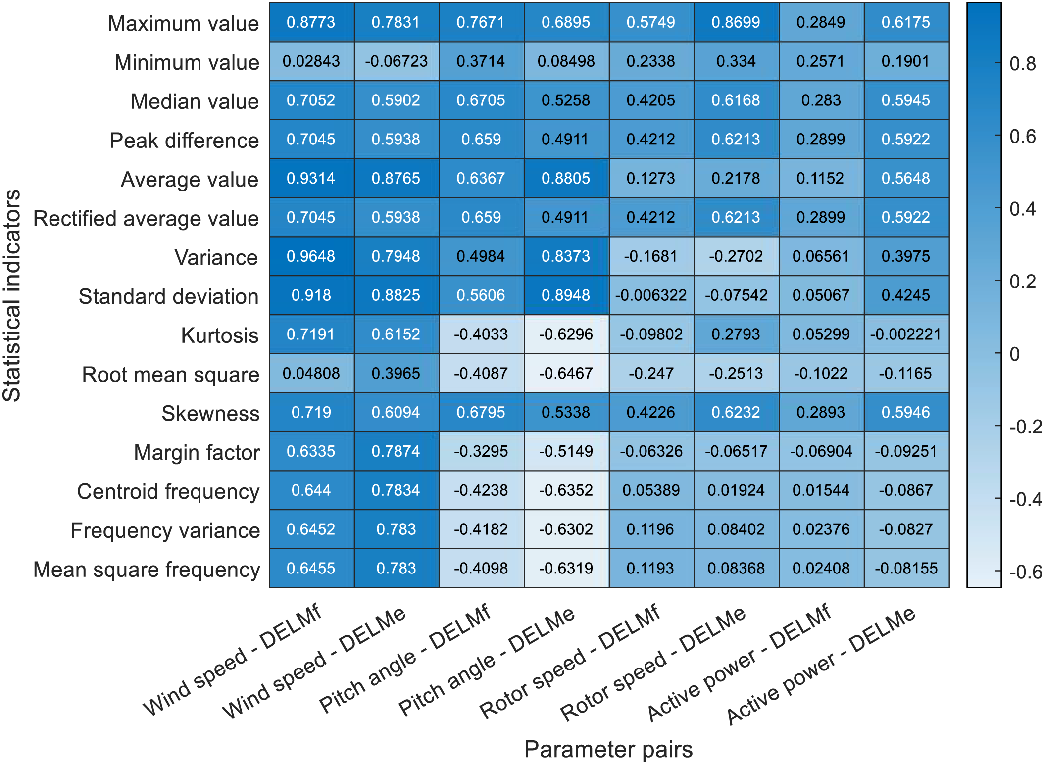
Figure 4: Correlation analysis between characteristic value and DEL
The correlation significance shown in the figure is significant at the bilateral 0.01 level. The correlations between different characteristics of different parameters and DEL are significantly different. Taking wind speed as an example, its average value, variance, and standard deviation all have a correlation with DELMf higher than 0.9, which shows that the average level and fluctuation of wind speed are the key factors leading to blade flapwise damage. Higher average wind speed and stronger turbulence will bring more significant blade flapwise damage. As for the damage caused by edgewise bending moment, the most significant related features of the pitch angle are the mean and standard deviation, which shows that frequent blade pitch changes or maintaining a large pitch angle will increase the damage caused by edgewise bending moment. In summary, the results of Fig. 4 are consistent with the laws of physics.
By setting the correlation coefficient to 0.6 as the threshold, 19 sets of feature parameters for DELMf and 25 sets of feature parameters for DELMe can be selected as input data for training the deep neural network, and the corresponding DEL as output data of the neural network. The specific parameter selection is shown in Table 5.
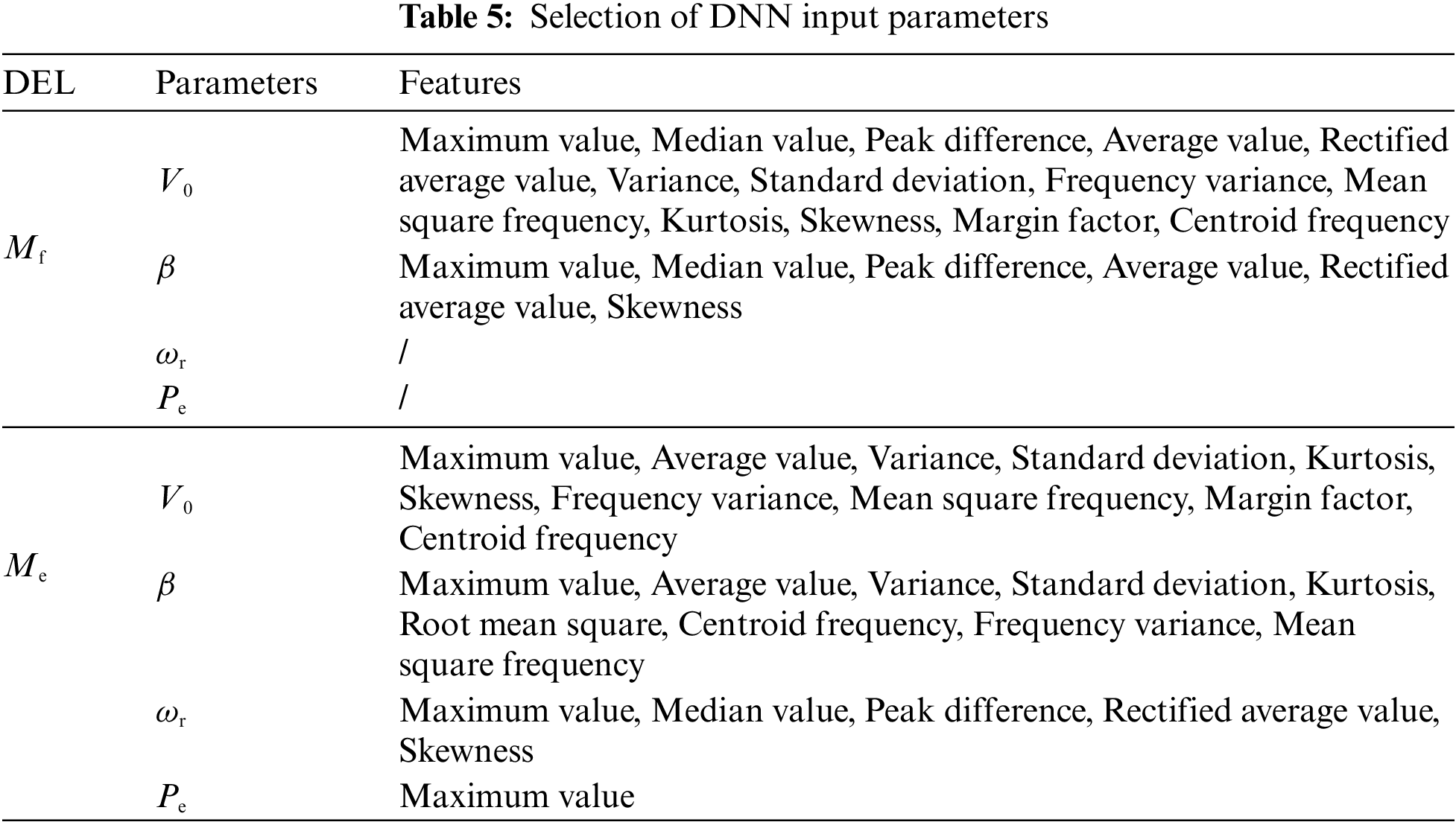
In Table 5, the DELs of the blade in both dimensions has obvious correlations with multiple features of V0 and β. The features of ωr and Pe have more influence on Me and have a lower correlation with Mf. The model is trained next based on the features selected in Table 5.
5.3 Effect of the Proposed DNN Model
During the DNN model training process, all 6000 simulation scenarios constructed in Section 4.1 were shuffled, 5800 working conditions were the training set, and the remaining 200 working conditions were used for test. After multiple attempts at parameters such as hidden layers, hidden layer nodes, and the activation function, the final structure selected is the DNN model in Table 6. The computer configuration used in the DNN training is as follows: i7-9700 CPU @ 3.00 GHz, 16.0 GB RAM. The training time is 32.7 s.

After training the DNN network based on the structure shown in Table 6, the accuracy was tested using 200 sets of test data, and the results are exhibited in Figs. 5 and 6.
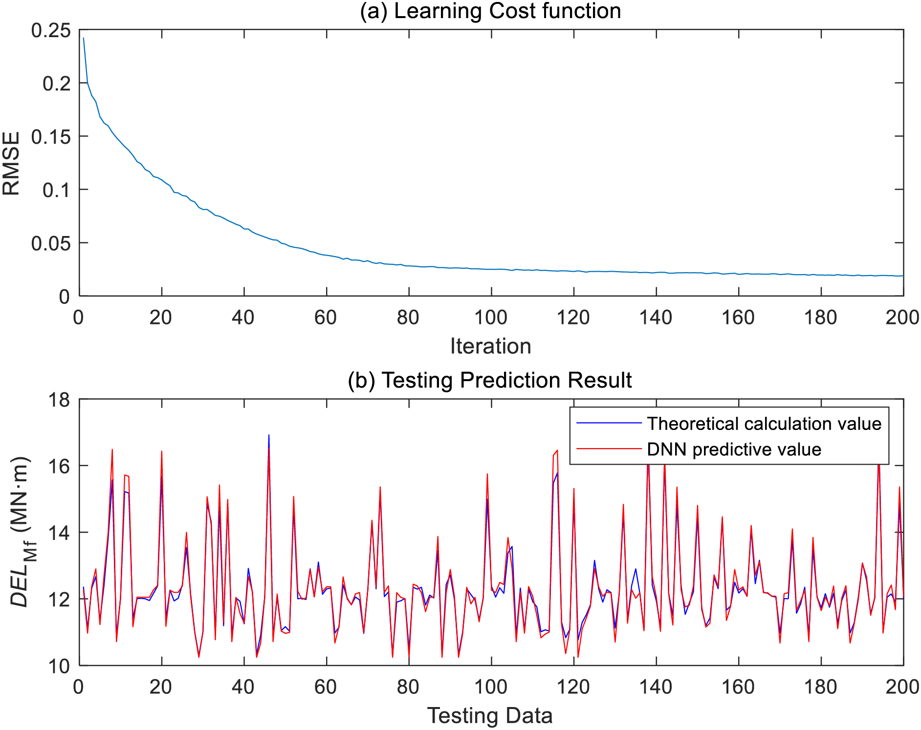
Figure 5: Training and testing results for DELMf
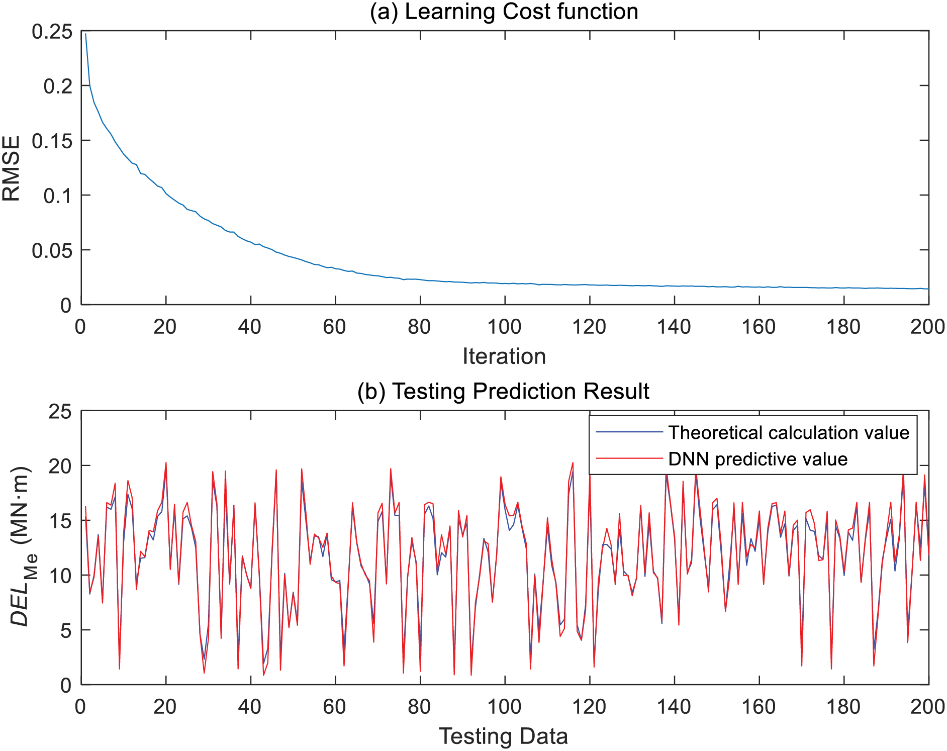
Figure 6: Training and testing results for DELMe
The results in Figs. 5 and 6 show that the constructed DNN model has reached a stable level after 200 training iterations. The trained DNN model has a good prediction ability for the DEL of the test group data, and the calculation accuracy of DELMf and DELMe reaches 98.8% and 91.6%, respectively. Moreover, when testing based on the trained model, it takes less than 0.02 s to calculate the blade DEL of the test scenario, which fully meets the requirements of real-time control and optimization.
5.4 Discussion on Generalization Ability
The results in Figs. 5 and 6 show that the constructed DNN model has a good prediction ability for the DEL of the in-sample working conditions. However, more out-of-sample working conditions may appear in the actual operation. Therefore, it is necessary to conduct further tests on out-of-sample working conditions to clarify the generalization ability of the proposed method. In addition, two other data-driven schemes are provided for comparison. C1 is designed based on [15] and uses the standard deviation of wind speed to construct a linear lookup table of two DELs of the blade. C2 is based on [17], using the average and standard deviation of V0, etc., as input for deep neural network training.
In this experiment, the average V0 is 10.85 m/s, the Ti is 13.27%, and the Pe is 1.165 MW, an out-of-sample condition inconsistent with the 6000 training and test conditions in Section 4.1. Under this condition, the DEL comparison results calculated by the proposed model, C1, and C2, are shown in Fig. 7. In the DELMf part, the results calculated by the three schemes are close to TCV, and the MAPE is above 98%. However, in the DELMe part, the calculation results of different schemes are significantly different, and the MAPE of the three schemes is 62%, 79%, and 83%, respectively. The proposed scheme also has a good calculation accuracy for out-of-sample working conditions.
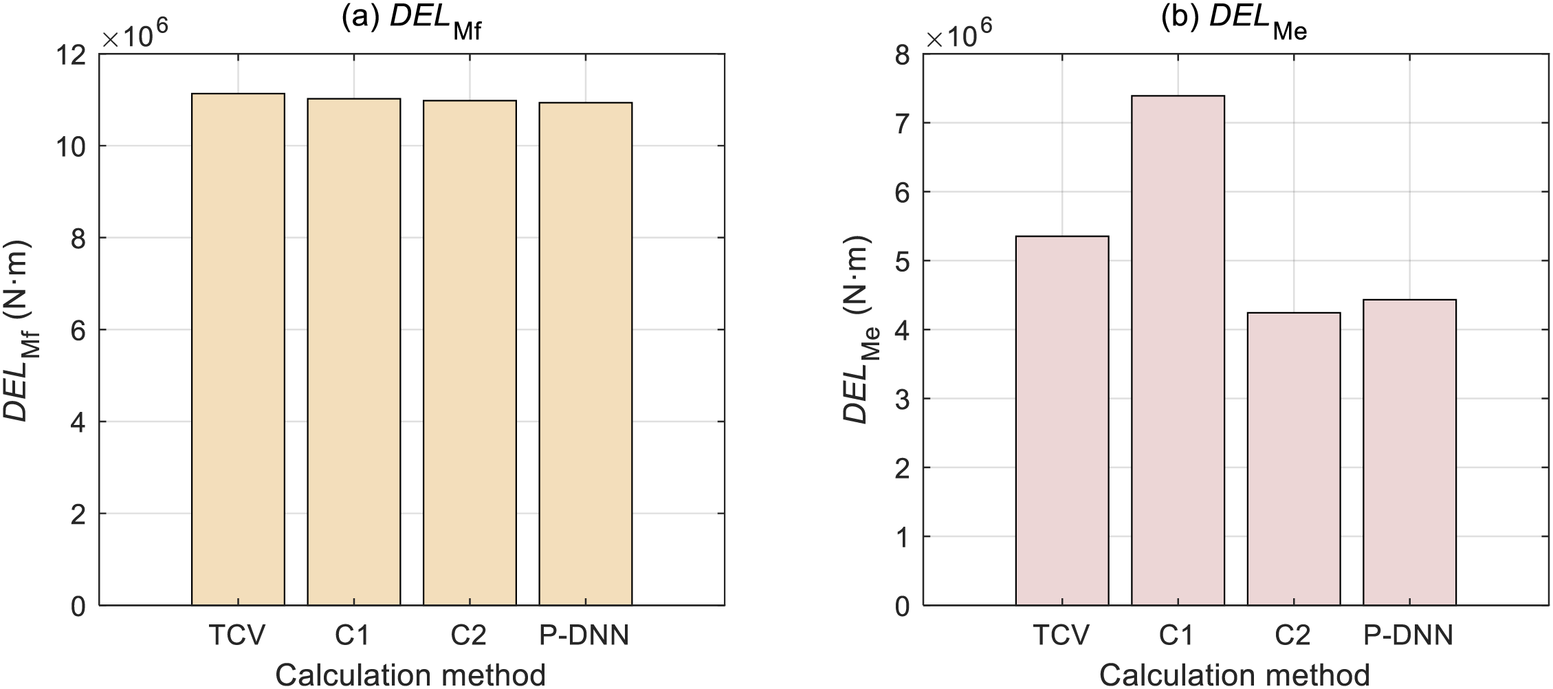
Figure 7: DEL prediction results of out-of-sample conditions under different schemes
For the calculation results in Fig. 7, the following discussion can be carried out:
First, the prediction accuracy of DELMf and DELMe for the same algorithm is inconsistent, and the prediction accuracy of DELMf is higher than DELMe. This is because the proposed scheme and the two schemes in the control group have more appropriate input selection for DELMf modeling. According to Fig. 4, the features used for DELMf calculation include the variance of wind speed, etc., and its correlation with DELMf is as high as more than 96%. In comparison, the correlation of modeling features for DELMe is less than 90%. Therefore, better feature selection will lead to better model accuracy.
Second, compared with the control method, the prediction accuracy of DELMe is higher in the proposed method. In particular, compared with C2, the same deep neural network modeling method is used, but the calculation accuracy of out-of-sample data is improved due to the improved input feature extraction method. Therefore, better feature selection will also lead to better model generalization ability.
Therefore, the deep neural network modeling method proposed in this paper has better description ability for nonlinear coupling relationships than the simple table lookup method, and the feature extraction process further improves model accuracy and generalization ability. If more appropriate features of parameters other than wind speed can be selected in future studies, the accuracy of the constructed model could be further improved.
This paper focuses on the modeling method of wind turbine blade load. Aiming at the problem of the theoretical calculation of wind turbine blade load being complex and requiring a large amount of calculation, a data-driven modeling scheme is proposed. The proposed scheme includes multiple steps: parameter selection, feature screening, scenario expansion, and model construction.
The developed solution avoids the time-consuming theoretical calculations using a large amount of data and the requirement to add additional sensors while having better generalization capabilities than existing solutions. Experimental results show that by extracting more relevant features for model training, the model constructed in this paper is more accurate than the existing data-driven load modeling method, and the accuracy for out-of-sample conditions is also higher than 80%.
At the same time, this study further highlights the importance of feature selection, especially for DELMe, whose data-driven modeling accuracy still has room for improvement. In future research, it is possible to consider using machine learning solutions to screen quasi-modeling parameters and autonomous learning of parameter features to improve the effect of the proposed model further.
Acknowledgement: The authors acknowledge the support from Energy and Electricity Research Center, Jinan University, Zhuhai, China.
Funding Statement: This paper is supported by Science and Technology Project funding from China Southern Power Grid Corporation No. GDKJXM20230245 (031700KC23020003).
Author Contributions: The authors confirm contribution to the paper as follows: study conception and design: Jianyong Ao; data collection: Yanping Li; analysis and interpretation of results: Shengqing Hu; draft manuscript preparation: Qi Yao and Songyu Gao. All authors reviewed the results and approved the final version of the manuscript.
Availability of Data and Materials: Data available on request from the authors.
Ethics Approval: Not applicable.
Conflicts of Interest: The authors declare that they have no conflicts of interest to report regarding the present study.
References
1. G. H. Liao and J. Z. Wu, “Study on determination method of fatigue testing load for wind turbine blade,” IOP Conf. Ser. Mater. Sci. Eng., vol. 224, no. 1, Jul. 2017, Art. no. 012040. doi: 10.1088/1757-899X/224/1/012040. [Google Scholar] [CrossRef]
2. W. Z. Guo, L. A. Zhang, L. Chao, W. S. Liu, and J. B. Tian, “Research on the follow-up control strategy of biaxial fatigue test of wind turbine blade based on electromagnetic excitation,” Energy Eng., vol. 120, no. 10, pp. 2307–2323, Sep. 2023. doi: 10.32604/ee.2023.030029. [Google Scholar] [CrossRef]
3. R. Y. Zhao, W. Z. Shen, T. Knudsen, and T. Bak, “Fatigue distribution optimization for offshore wind farms using intelligent agent control,” Wind Energy, vol. 15, no. 7, pp. 927–944, Oct. 2012. doi: 10.1002/we.1518. [Google Scholar] [CrossRef]
4. H. Liao et al., “Active power dispatch optimization for offshore wind farms considering fatigue distribution,” Renew Energy, vol. 151, no. 1, pp. 1173–1185, May 2020. doi: 10.1016/j.renene.2019.11.132. [Google Scholar] [CrossRef]
5. G. H. Wang, J. H. Wang, X. M. Huang, L. A. Zhang, and W. S. Liu, “An advanced control strategy for dual-actuator driving system in full-scale fatigue test of wind turbine blades,” Energy Eng., vol. 119, no. 4, pp. 1649–1662, Dec. 2021. doi: 10.32604/ee.2022.019695. [Google Scholar] [CrossRef]
6. Y. Yuan and J. Tang, “Adaptive pitch control of wind turbine for load mitigation under structural uncertainties,” Renew Energy, vol. 105, no. 4, pp. 483–494, May 2017. doi: 10.1016/j.renene.2016.12.068. [Google Scholar] [CrossRef]
7. S. K. Liu, Z. U. Gao, R. N. Su, M. M. Yan, and J. W. Wang, “Impact of blade-flapping vibration on aerodynamic characteristics of wind turbines under yaw conditions,” Energy Eng., vol. 121, no. 8, pp. 2213–2229, Jul. 2024. doi: 10.32604/ee.2024.049616. [Google Scholar] [CrossRef]
8. Q. F. Lang, Y. Q. Zheng, T. C. Cui, C. L. Shi, and H. Y. Zhang, “Nonlinear flap-wise vibration characteristics of wind turbine blades based on multi-scale analysis method,” Energy Eng., vol. 121, no. 2, pp. 483–498, Jan. 2024. doi: 10.32604/ee.2023.042437. [Google Scholar] [CrossRef]
9. B. Biegel, D. Madjidian, V. Spudić, A. Rantzer, and J. Stoustrup, “Distributed low-complexity controller for wind power plant in derated operation,” in IEEE Int. Conf. Control Appl. (CCA), Aug. 2013, pp. 146–151. [Google Scholar]
10. T. Knudsen, T. Bak, and M. Svenstrup, “Survey of wind farm control-power and fatigue optimization: Survey of wind farm control,” Wind Energy, vol. 18, no. 8, pp. 1333–1351, Aug. 2015. doi: 10.1002/we.1760. [Google Scholar] [CrossRef]
11. H. J. Sutherland, On the Fatigue Analysis of Wind Turbines. Livermore, CA, USA: Sandia National Lab, Jun. 1999. [Google Scholar]
12. H. L. Liu, H. J. Liu, C. C. Zhu, and Y. B. Ge, “Influence of load spectrum on contact fatigue damage of a case carburized wind turbine gear,” Eng. Fail. Anal., vol. 119, Jan. 2021, Art. no. 105005. doi: 10.1016/j.engfailanal.2020.105005. [Google Scholar] [CrossRef]
13. L. Buhl Marshall, MCrunch User’s Guide for Version 1. 00. Denver, CO, USA: National Renewable Energy Laboratory, 2008. [Google Scholar]
14. Q. Yao, Y. Hu, H. Deng, Z. L. Luo, and J. Z. Liu, “Two-degree-of-freedom active power control of megawatt wind turbine considering fatigue load optimization,” Renew Energy, vol. 162, pp. 2096–2112, Dec. 2020. doi: 10.1016/j.renene.2020.09.137. [Google Scholar] [CrossRef]
15. G. S. Sudharsan, K. Natarajan, S. G. Rahul, and A. Kumar, “Active power control in horizontal axis wind turbine considering the fatigue structural load parameter using psuedo adaptive-model predictive control scheme,” Sustain. Energy Techn., vol. 57, Jun. 2023, Art. no. 103166. doi: 10.1016/j.seta.2023.103166. [Google Scholar] [CrossRef]
16. E. J. Alvarez and A. P. Ribaric, “An improved-accuracy method for fatigue load analysis of wind turbine gearbox based on SCADA,” Renew Energy, vol. 115, pp. 391–399, Jan. 2018. doi: 10.1016/j.renene.2017.08.040. [Google Scholar] [CrossRef]
17. B. H. Zhang, M. Soltani, W. H. Hu, P. Hou, Q. Huang and Z. Chen, “Optimized power dispatch in wind farms for power maximizing considering fatigue loads,” IEEE Trans. Sustain. Energy, vol. 9, no. 2, pp. 862–871, Apr. 2018. doi: 10.1109/TSTE.2017.2763939. [Google Scholar] [CrossRef]
18. J. Yang, S. Y. Zheng, D. R. Song, M. Su, X. B. Yang and Y. H. Joo, “Data-driven modeling for fatigue loads of large-scale wind turbines under active power regulation,” Wind Energy, vol. 24, no. 6, pp. 558–572, Jun. 2021. doi: 10.1002/we.2589. [Google Scholar] [CrossRef]
19. X. X. Yin, W. C. Zhang, Z. S. Jiang, and L. Pan, “Data-driven multi-objective predictive control of offshore wind farm based on evolutionary optimization,” Renew Energy, vol. 160, pp. 974–986, Nov. 2020. doi: 10.1016/j.renene.2020.05.015. [Google Scholar] [CrossRef]
20. D. Pérez-Campuzano, E. G. D. Heras-Carbonell, C. Gallego-Castillo, and A. Cuerva, “Modelling damage equivalent loads in wind turbines from general operational signals: Exploration of relevant input selection methods using aeroelastic simulations,” Wind Energy, vol. 21, no. 6, pp. 441–459, Jun. 2018. doi: 10.1002/we.2171. [Google Scholar] [CrossRef]
21. F. D. Santos, N. Noppe, W. Weijtjens, and C. Devriendt, “Farm-wide interface fatigue loads estimation: A data-driven approach based on accelerometers,” Wind Energy, vol. 27, no. 4, pp. 321–340, Apr. 2024. doi: 10.1002/we.2888. [Google Scholar] [CrossRef]
22. Q. Yao, B. Ma, T. Y. Zhao, Y. Hu, and F. Fang, “Optimized active power dispatching of wind farms considering data-driven fatigue load suppression,” IEEE Trans. Sustain. Energy, vol. 14, no. 1, pp. 371–380, Jan. 2023. doi: 10.1109/TSTE.2022.3213992. [Google Scholar] [CrossRef]
23. X. Liu and W. Zhang, “Physics-informed deep learning model in wind turbine response prediction,” Renew Energy, vol. 185, no. 7, pp. 932–944, Feb. 2022. doi: 10.1016/j.renene.2021.12.058. [Google Scholar] [CrossRef]
24. L. D. Avendaño-Valencia, I. Abdallah, and E. Chatzi, “Virtual fatigue diagnostics of wake-affected wind turbine via Gaussian Process Regression,” Renew Energy, vol. 170, pp. 539–561, Jun. 2021. doi: 10.1016/j.renene.2021.02.003. [Google Scholar] [CrossRef]
25. F. C. Mehlan, J. Keller, and A. R. Nejad, “Virtual sensing of wind turbine hub loads and drivetrain fatigue damage,” Forsch. Ingenieurwes., vol. 87, no. 1, pp. 207–218, Mar. 2023. doi: 10.1007/s10010-023-00627-0. [Google Scholar] [CrossRef]
26. S. A. El-Shahat, G. J. Li, F. Lai, and L. Fu, “Investigation of parameters affecting horizontal axis tidal current turbines modeling by blade element momentum theory,” Ocean Eng., vol. 202, Apr. 2020, Art. no. 107176. doi: 10.1016/j.oceaneng.2020.107176. [Google Scholar] [CrossRef]
27. A. Erduman, B. Uzunoğlu, B. Kekezoğlu, and A. Durusu, “Mesoscale wind farm placement via linear optimization constrained by power system and techno-economics,” J. Mod Power Syst. Cle., vol. 9, no. 2, pp. 356–366, Mar. 2021. doi: 10.35833/MPCE.2019.000150. [Google Scholar] [CrossRef]
28. J. S. Nielsen, L. Miller-Branovacki, and R. Carriveau, “Probabilistic and risk-informed life extension assessment of wind turbine structural components,” Energies, vol. 14, no. 4, Feb. 2021, Art. no. 821. doi: 10.3390/en14040821. [Google Scholar] [CrossRef]
29. A. Natarajan, “Damage equivalent load synthesis and stochastic extrapolation for fatigue life validation,” Wind Energy Sci., vol. 7, no. 3, pp. 1171–1181, Jun. 2022. doi: 10.5194/wes-7-1171-2022. [Google Scholar] [CrossRef]
30. Y. Zhao, Y. Y. Shen, Y. M. Zhu, and J. J. Yao, “Forecasting wavelet transformed time series with attentive neural networks,” in 2018 IEEE Int. Conf. Data Mining (ICDM), Singapore, 2018, pp. 1452–1457. [Google Scholar]
31. H. R. Ahmadi, K. Momeni, and Y. Jasemnejad, “A new algorithm and damage index for detection damage in steel girders of bridge decks using time-frequency domain and matching methods,” Structures, vol. 61, no. 1, Mar. 2024, Art. no. 106035. doi: 10.1016/j.istruc.2024.106035. [Google Scholar] [CrossRef]
32. A. Field, Discovering Statistics Using IBM SPSS Statistics. Thousand Oaks, CA, USA: Sage Publications Ltd, 2024. [Google Scholar]
33. M. Reyad, A. M. Sarhan, and M. Arafa, “A modified Adam algorithm for deep neural network optimization,” Neural Comput. Appl., vol. 35, no. 23, pp. 17095–17112, Aug. 2023. doi: 10.1007/s00521-023-08568-z. [Google Scholar] [CrossRef]
34. M. Topor, “Real time wind farm emulation using simwindfarm toolbox,” AIP Conf. Proc., vol. 1738, Jun. 2016, Art. no. 410003. doi: 10.1063/1.4952204. [Google Scholar] [CrossRef]
35. J. Jonkman, S. Butterfield, W. Musial, and G. Scott, Definition of a 5-MW Reference Wind Turbine for Offshore System Development. Golden, CO, USA: National Renewable Energy Lab, 2009. [Google Scholar]
36. K. T. Fang and Y. Wang, Number-Theoretic Methods in Statistics. China: Science Press (in Chinese1996. [Google Scholar]
Cite This Article
 Copyright © 2024 The Author(s). Published by Tech Science Press.
This work is licensed under a Creative Commons Attribution 4.0 International License , which permits unrestricted use, distribution, and reproduction in any medium, provided the original work is properly cited.


 Submit a Paper
 Propose a Special lssue
 View Full Text
 Download PDF
 Downloads
 Citation Tools