Photovoltaic Power Generation Power Prediction under Major Extreme Weather Based on VMD-KELM

Nomenclature

1  Introduction

The global expansion of photovoltaic power generation is crucial for combating climate change and advancing sustainable development. Reports from the International Energy Agency (IEA) and other energy regulators indicate a rapid increase in installed capacity worldwide [1]. In China, the United States, and Europe, photovoltaic power generation has emerged as a significant new electricity source. Many countries have implemented policies to support renewable energy development, including subsidies, tax incentives, and green credits. Additionally, improvements and developments in solar cell performance, cost reduction efforts, advancements in battery energy storage technology, and the implementation of carbon emission restrictions for numerous companies will create new growth opportunities for the photovoltaic market, solidifying its position in the global energy market [2].

Large-scale photovoltaic power generation connected to the grid can have a negative impact on the power system [3]. The integration of large-scale photovoltaic systems into the power grid can affect the frequency stability of the grid. Unlike hydropower or thermal power plants, which traditionally handle frequency adjustments, photovoltaic power generation is unable to regulate frequency, leading to challenges in coordinating frequency regulation within the power system. Additionally, a significant number of photovoltaic systems connected to the grid may result in issues such as inadequate reactive power support, noticeable voltage stability concerns, and heightened risks of exceeding limits. The intermittent and fluctuating nature of photovoltaic power generation makes it challenging to predict active power output, affecting the frequency regulation of the grid. Weather conditions greatly influence photovoltaic power generation, leading to significant voltage fluctuations during startup and shutdown, as well as output variations. This can result in improper reactive power flow, deteriorating power quality and possibly altering power flow direction.

As global warming intensifies, the energy balance of the climate system shifts, resulting in more frequent and intense extreme weather events. The impact of such weather on photovoltaic power is especially severe. Dust storms, heavy rain, or hail can significantly reduce solar power generation by either damaging solar panels or obstructing sunlight exposure, thereby decreasing efficiency. Moreover, prolonged high temperatures can lower the efficiency of photovoltaic panels. Failure to accurately predict these changes may result in a mismatch between power system load and supply, leading to increased system operation instability. This, in turn, can prompt dispatchers to frequently adjust dispatch plans to accommodate sudden changes in power supply. Ensuring the stable operation of the power grid and the efficient allocation of resources requires precise short-term prediction of photovoltaic power generation during major extreme weather conditions [4–7].

Photovoltaic power forecasting is typically categorized into ultra-short-term forecasting, short-term forecasting, medium-term forecasting, and long-term forecasting based on different time ranges. Current research primarily focuses on ultra-short-term and short-term forecasting. Ultra-short-term forecasting involves predicting photovoltaic power within the next few minutes to hours, utilizing meteorological data from satellite images, weather radar, and ground weather stations. This is achieved through physical models, statistical methods, and machine learning techniques, including support vector machines (SVMs) [8,9] and artificial neural networks (ANNs) [10]. Short-term forecasting, on the other hand, covers predictions from hours to days, combining detailed meteorological forecasts and employing more complex statistical and machine learning methods such as regression analysis, time series analysis, and ensemble learning. Ultra-short-term forecasting provides higher-precision results due to its shorter time range and reliance on near-real-time data and rapidly changing environmental factors. In contrast, short-term forecasts rely more on comprehensive weather forecasts and historical data analysis, facing greater uncertainty and potentially lower forecast accuracy.

The primary objective of this research is to investigate ultra-short-term photovoltaic power forecasting during major extreme weather conditions, utilizing machine learning techniques and creating a deep learning model that integrates variational mode decomposition (VMD) with kernel extreme learning machine (KELM). This model can efficiently break down time series data, enabling a better understanding of nonlinear and non-stationary features within the data, and ultimately enhancing the accuracy of the forecast model. The model is specifically tailored to predict photovoltaic power generation in Nanjing during major extreme weather events.

The key contributions of this study are outlined as follows:

•   A hybrid prediction model that combines the Variational Mode Decomposition (VMD) algorithm with the Kernel Extreme Learning Machine (KELM) is proposed for forecasting photovoltaic power generation during major extreme weather conditions.

•   The network prediction model of this paper is compared and analyzed alongside other models to demonstrate the superior accuracy and suitability of the proposed model for predicting photovoltaic power in local weather conditions.

•   This study examines the accuracy of photovoltaic power prediction in four different major extreme weather scenarios and provides an analysis of the key factors that influence photovoltaic power output.

2  Literature Review

Current research on photovoltaic power prediction methods is commonly categorized into three groups: methods based on physical models, statistical models, and machine learning. Physical model-based prediction methods utilize the physical characteristics and environmental parameters of photovoltaic cells to forecast power output, requiring a comprehensive understanding and simulation of how photovoltaic cells respond to environmental factors. This includes predicting solar radiation, photovoltaic module temperature, and ultimately photovoltaic power output using an established photovoltaic cell model. These methods demand high accuracy in modeling and quality input data, typically incorporating other prediction methods for improved prediction accuracy. Statistical model-based methods, on the other hand, rely on historical data to predict future photovoltaic power by establishing mathematical relationships between meteorological conditions and power output. Time series models, like the autoregressive model (AR), moving average model (MA), and autoregressive integrated moving average (ARIMA), are commonly employed to analyze and predict time-correlated data, often integrating decision trees, random forests, and gradient boosting machines to enhance prediction accuracy. In recent years, machine learning-based methods have gained popularity for their ability to significantly improve the accuracy of Photovoltaic (PV) power predictions. These methods often leverage technical models such as Long Short-Term Memory Networks (LSTMs) [11,12], Support Vector Machines (SVMs), and Convolutional Neural Networks (CNNs) [13] to forecast photovoltaic power.

Various domestic and international researchers have utilized machine learning and combined prediction methods to investigate the prediction of new energy power. In [14], weather images above photovoltaic power stations are analyzed using a combination of convolutional neural networks (CNNs) and long short-term memory (LSTM) for short-term predictions of photovoltaic power. Reference [15] employs support vector machine modeling to enhance the accuracy of predictions solar and wind energy resources. Reference [16] introduces an ESN (Echo State Network)-KELM dual-core prediction model, optimizing its parameters with the Archimedean optimization method to improve accuracy. In [17], LSTM is used to extract time features from input data, establishing a relationship between features and output based on Temporal Convolutional Network (TCN) for multi-step prediction of photovoltaic output under various conditions. Reference [18] proposes an advanced photovoltaic power prediction model that combines TimeGAN, and k-means clustering algorithm based on soft dynamic time warping, CNN, and Gate Recurrent Unit (GRU) in a unified framework for the accurate prediction of photovoltaic output under different weather conditions.

Numerous studies have focused on meteorological factors for predicting various types of power generation units, delving into the extraction and classification of meteorological data features. For instance, in [19], numerical weather forecast data are utilized with a focus on the hourly temperature trend as a crucial predictor for predicting hourly photovoltaic output. Reference [20] employs the grey relational analysis method to identify impactful meteorological factors for distributed photovoltaic power generation, using the XGBoost algorithm to train selected data sets and incorporating weather forecasts for prediction. In [21], the Pearson correlation coefficient method and kmeans++ are used to cluster meteorological features for obtaining precise similar days, integrating the IXGBoost-KELM algorithm for short-term photovoltaic output predictions. Reference [22] uses heat maps to identify environmental factor input variables and proposed a novel network prediction model: an ensemble empirical mode decomposition (EEMD) was used to decompose the data and combined with the VMD-BiLSTM prediction algorithm to accurately forecast the target. Furthermore, in [23], atmospheric turbidity, relative humidity, and solar irradiance are selected as clustering feature vectors. By applying an improved fuzzy c-means clustering method to meteorological data, the genetic algorithm planning system (GAPS) and radial basis function (RBF) joint algorithm are used to enhance the accuracy of photovoltaic output predictions. Reference [24] utilizes pixels from satellite images obtained from the European Organization for the Exploitation of Meteorological Satellites (EUMETSAT) to transform them into structured data arrays. These arrays are then used as exogenous inputs in the algorithm to enhance the precision of solar irradiance prediction.

There is a lack of research on predicting photovoltaic power under extreme weather conditions. The limited availability of meteorological data and insufficient machine learning training contribute to lower prediction accuracy. Additionally, the complexity of meteorological factors and the frequent changes in meteorological characteristics in extreme weather make it challenging to provide consistent predictions for photovoltaic power generation.

Based on this current situation, this paper presents a photovoltaic power generation power prediction method for major extreme weather conditions using the VMD-KELM network prediction model. Initially, a grey relational analysis was conducted to assess the impact of meteorological factors on photovoltaic power output during extreme weather events. Subsequently, the GMM clustering algorithm was applied to train and process meteorological data based on key meteorological characteristics, focusing on key characteristics such as dust storms, thunderstorms, hail solid precipitation, and snowstorms. The VMD-KELM network prediction model was then utilized to forecast photovoltaic output, followed by an analysis of the changes and factors influencing photovoltaic output under major extreme weather conditions.

3  Analysis of Factors Affecting Photovoltaic Power Generation

Since many meteorological factors have a significant impact on the output of photovoltaic power, this section uses the grey relational analysis method to assess the influence of different meteorological factors on the output of photovoltaic power. This aims to identify the major factors that significantly impact photovoltaic power output. An exemplary analysis was also conducted under the meteorological conditions of thunderstorm weather.

3.1 Grey Relational Analysis

The grey relational analysis is a technique within grey system theory designed to address uncertainties in a system. It assesses the correlation strength between different factors by measuring their similarity. The fundamental concept of this method revolves around comparing the similarity of sequences. When two sequences exhibit similar developmental trends, their correlation is considered high; otherwise, it is considered low. The basic steps of grey relational analysis include the following:

1. Normalization

This article employs range normalization to process the data, effectively removing the influence of differing scales and variations in magnitude across different indicators. The standardized data is then transformed into the [0, 1] interval using the following calculation formula:

x∗=x−min(x)max(x)−min(x)(1)

where x is the original data, min(x) and max(x) are the minimum and maximum values of the data sequence, respectively.

2. Calculation of correlation coefficients

The correlation coefficient is an indicator of the similarity between the comparison series and the reference series and is calculated as follows:

ξ(k)=minimink|x0(k)−xi(k)|+ρmaximaxk|x0(k)−xi(k)||x0(k)−xi(k)|+ρmaximaxk|x0(k)−xi(k)|(2)

where x0(k) is the value of the reference sequence at the k−th point, xi(k) is the value of the i−th comparison sequence at the k−th point, mini, mink and maxi, maxk represent the minimum and maximum differences of all sequences at all points, respectively. ρ is the resolution coefficient, used to adjust the sensitivity of the correlation coefficient.

3. Calculate grey relation grade

The correlation coefficients are averaged over the points and the result is the correlation, which is given by the formula:

ri=1n∑k=1nξi(k)(3)

where n is the length of the sequence.

3.2 Examples of Analysis and Results

Various meteorological factors can influence photovoltaic power generation, emphasizing the importance of selecting appropriate environmental parameters for prediction models. For instance, in the case of heavy rain, data from 0:00 on 23 June 2023 to 23:00 on 24 June 2023 in Nanjing City were analyzed using an averaging processing method with a resolution coefficient of 0.5. The x-axis denotes the time periods of data collection, with a resolution of 1 h, totaling 47 data points, while the y-axis represents the grey relational coefficient. Higher values indicate a greater impact on power generation. The correlation coefficients of 11 meteorological evaluation factors on photovoltaic output results are illustrated in Fig. 1; Table 1 displays the grey relational results.

Figure 1: Connected graph

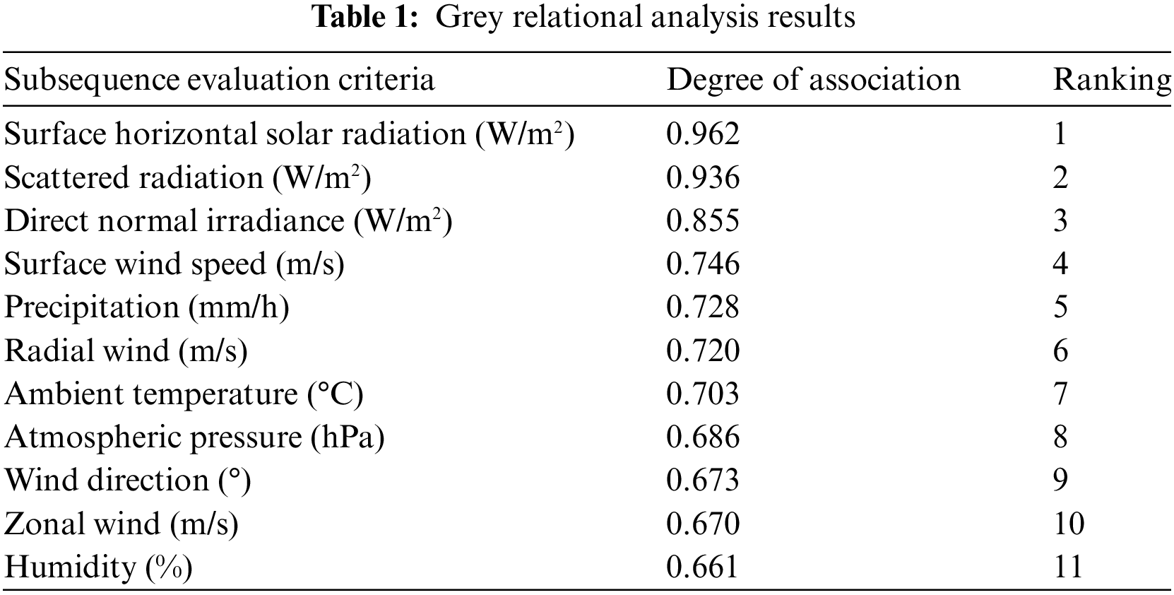
Under extreme weather conditions, different weather types have different influencing factors on photovoltaic power generation, and the degree of influence of meteorological factors will also differ. Therefore, this article conducts a grey relational analysis on the impact of several meteorological factors on photovoltaic power generation under extreme weather, such as heavy rain, snowstorms, dust storms, typhoons, high temperatures, drought, etc. For other types of extreme weather, the calculation steps and processes for grey relational degree are consistent with those described in the heavy rain example above. Finally, these results were combined, and the top six factors with the greatest impact were identified, which were: surface horizontal solar radiation, ambient temperature, air pressure, wind speed, relative humidity, and cloud cover.

4  Meteorological Clustering Types

Short-term photovoltaic power prediction is based on historical output power data, numerical weather prediction, and actual meteorological data, establishing a model to predict photovoltaic output power for the next 24 h. Since the photovoltaic power prediction in this paper is conducted under extreme weather conditions, the data is characterized by significant numerical fluctuations and frequent changes, making data reliability particularly important. This paper considers solar radiation, ambient temperature, and wind speed as the main meteorological factors affecting photovoltaic output power. A meteorological clustering model is proposed, which uses the Gaussian Mixture Model (GMM) clustering algorithm to train the data, gradually increasing the likelihood probability of the data. Meteorological data points are classified based on their probabilities in various Gaussian distributions. By analyzing the characteristic differences between different clusters, the data is divided into different types of weather data. Then, based on similar day samples, a photovoltaic power generation model is established, providing the data foundation for subsequent photovoltaic power prediction.

The steps for using the GMM clustering algorithm to classify meteorological clusters are as follows:

(a) Establish an initial sample set of meteorological data that follows a mixed Gaussian distribution.

The probability density function of its individual Gaussian distribution is represented as follows:

𝒩(x|μ,Σ)=1(2π)d/2|Σ|1/2e(−12(x−μ)TΣ−1(x−μ))(4)

where x is a d-dimensional data point; μ is the mean vector; Σ is the covariance matrix; |Σ| is the determinant of the covariance matrix. d is the dimension of the random vector.

The probability density function of a Gaussian mixture distribution can be represented as the weighted sum of each individual Gaussian distribution. The mathematical expression for this is as follows:

p(x)=∑k=1Kπk𝒩(x|μk,Σk)(5)

where πk, μk, and Σk are the mixing coefficient, mean, and covariance matrix of the k−th Gaussian distribution, respectively; k is the number of Gaussian distributions; 𝒩(x|μk,Σk) is the probability density function of the k−th Gaussian distribution;

(b) Initialize the parameters of the GMM model, such as the mean, covariance, and mixing coefficients.

(c) Estimate GMM parameters using the Expectation-Maximization (EM) algorithm, which includes using the Expectation step (E-step) to calculate the probability of each data point belonging to each Gaussian distribution, and the Maximization step (M-step) to update model parameters.

Use the EM algorithm to maximize the log-likelihood function of the observed data, with the formula for the log-likelihood function shown as follows:

log⁡p(X|π,μ,Σ)=∑i=1Nlog⁡(∑k=1Kπk𝒩(xi|μk,Σk))(6)

where X is the observed dataset and N is the number of data points.

During the Expectation step (E-step), calculate the probability of each data point belonging to each Gaussian distribution. For each data point xi, compute its posterior probability for each cluster k, with the formula shown as follows:

γ(zik)=πk𝒩(xi|μk,Σk)∑j=1Kπj𝒩(xi|μj,Σj)(7)

where 𝒩(xi|μk,Σk) is the probability density function of the data point xi with respect to the Gaussian distribution k.

Then, update the parameters for each cluster in the Maximization step (M-step), with the update formulas shown as follows:

πknew=1N∑i=1Nγ(zik)(8)

μknew=∑i=1Nγ(zik)xi∑i=1Nγ(zik)(9)

Σknew=∑i=1Nγ(zik)(xi−μknew)(xi−μknew)T∑i=1Nγ(zik)(10)

Repeat Eqs. (7) to (10) until the change in parameters is smaller than the predetermined computational accuracy or the maximum number of iterations is reached. The final computational result will converge.

(d) Processing meteorological data results in five major types of meteorological data categories, as shown in Table 2 below.

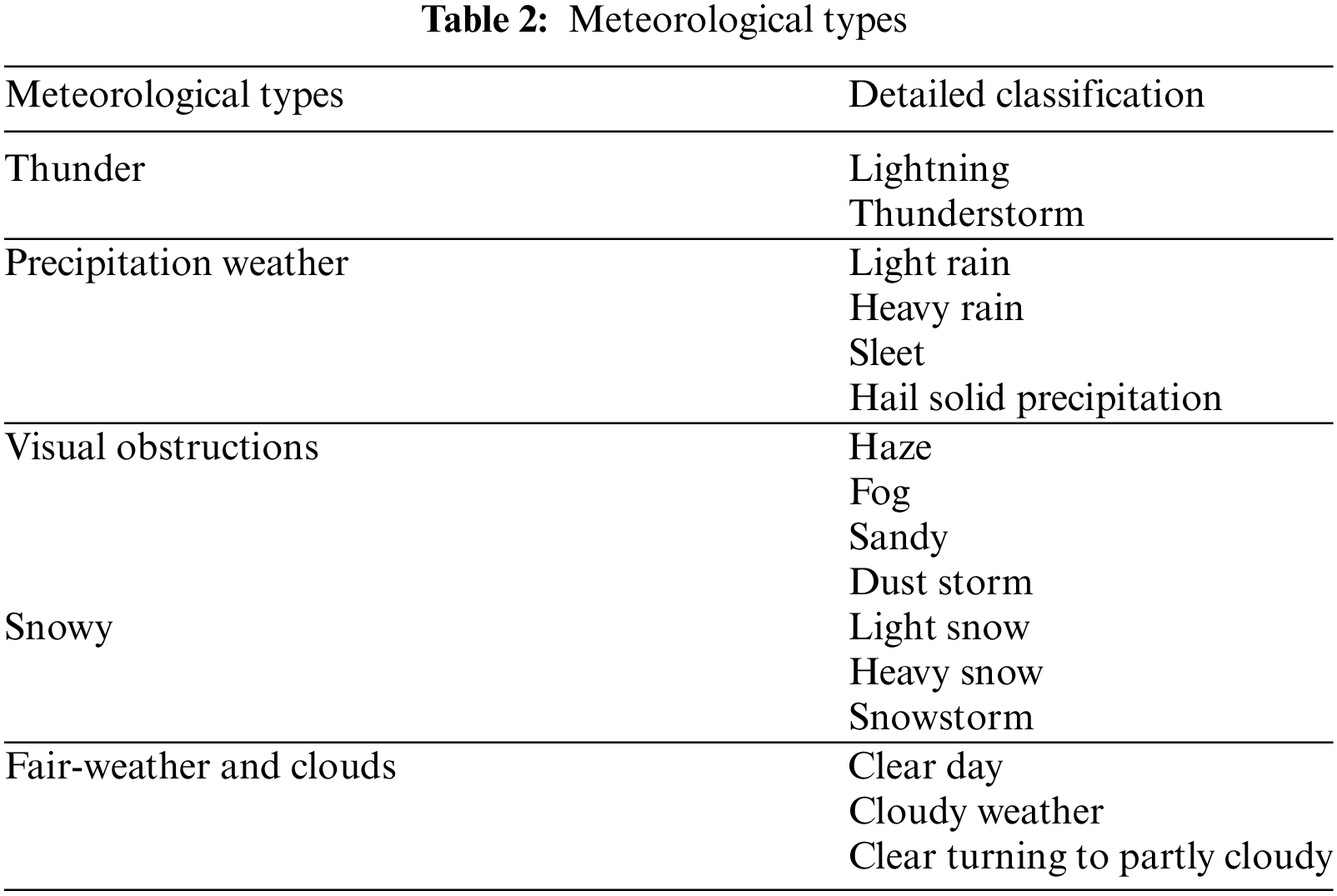
This study examines meteorological clusters during major extreme weather events, focusing on thunderstorms, hail solid precipitation, snowstorms, and dust storms as four types of weather, with clear day serving as the control group. It then establishes samples of similar photovoltaic power days under different major extreme weather conditions. The subsequent parts of this paper will use the data selected for the four types of extreme weather—thunderstorms, hail solid precipitation, snowstorms, and dust storms—and used to train and test the VMD-KELM prediction model separately for each type to ensure the reliability of the forecasting results.

5  Photovoltaic Power Prediction Method Based on Meteorological Clustering and Typing

5.1 VMD-KELM Network Prediction Model

The primary objective of the VMD-KELM network prediction model is to utilize VMD (variational mode decomposition) to break down the signal into individual intrinsic modal functions (IMFs) with a predetermined number of modes. Subsequently, the model leverages KELM (kernel extreme learning machine) to address complex spatial problems by transforming them into high-dimensional inner product operation problems. Each scale’s modal function is then modeled and predicted, and the resulting sub-sequence prediction is reconstructed to yield the final power prediction outcome. This methodology can enhance the accuracy of photovoltaic output predictions significantly.

5.1.1 Variational Mode Decomposition (VMD)

The primary objective of the VMD-KELM network prediction model is to utilize VMD (variational mode decomposition) to break down the signal into individual modal functions with a predetermined number of modes. Subsequently, the model leverages KELM (kernel extreme learning machine) to address complex spatial problems by transforming them into high-dimensional inner product operation problems. Each scale’s modal function is then modeled and predicted, and the resulting sub-sequence prediction is reconstructed to yield the final power prediction outcome. This methodology has been proven to significantly enhance the accuracy of photovoltaic output predictions.

(a) By setting the maximum number of iterations and iteration tolerance, the original signal f is decomposed into k intrinsic IMFs with a certain frequency band. Each modal function is subjected to Hilbert transform for signal analysis and its unilateral spectrum is obtained.

(b) An exponential term is introduced to adjust the center frequency ωk of each modal function uk(t), and the spectrum of each mode is modulated accordingly to adapt to the fundamental frequency bandwidth.

(c) The fundamental frequency bandwidth of each modal function uk(t) is estimated by calculating the gradient two-norm of the demodulated signal, and the constraints of its variational model are constructed:

min{uk},{ωk}∑k=1K‖∂t[(δ(t)+jω^k2)∗uk(t)]‖22(11)

s.t.f(t)−∑k=1Kuk(t)=0(12)

where {uk} represents the k−th modal function; {ωk} is the corresponding center frequency; δ(t) is the unit impulse function; ∗ represents convolution operation; ∂t represents the derivative of time.

(d) To ensure the accuracy and integrity of the original signal reconstructed by the sum of all intrinsic IMFs decomposed by VMD, the Lagrangian multiplier method is needed to integrate the above constraints into the optimization problem, and a Lagrangian function is constructed to transform the original problem into an unconstrained problem. The Lagrangian function is as follows:

L=∑k=1K‖∂t[(δ(t)+jω^k2)∗uk(t)]‖22+λ(t)[f(t)−∑k=1Kuk(t)](13)

where λ(t) is a Lagrangian multiplier, which is a time function used to enforce signal reconstruction constraints.

(e) Iterative update of parameters in the solution process.

Fix ω^k and λ(t), update uk(t): update each IMF to minimize the Lagrangian function.

Fix uk(t) and λ(t), update ω^k: update the center frequency of each IMF to further minimize the Lagrangian function.

Update the Lagrangian multiplier λ(t): Finally, the Lagrangian multiplier is updated to meet the signal reconstruction constraints.

The above iteration process is continued until the difference between all IMFs and the original signal is less than the set calculation accuracy, or the maximum number of iterations is reached.

5.1.2 Kernel Extreme Learning Machine (KELM)

KELM is a kernel method based on the optimization of traditional Extreme Learning Machine (ELM). After mapping the original data to the high-dimensional kernel space, the dot product operation between samples can be directly performed using the kernel function. Therefore, the relationship between samples has a direct causal connection to the selection of kernel function. The structure of the KELM model is shown in Fig. 2.

•   Input layer.

The input layer is responsible for receiving the original data, which consists of n features. These features can be expressed as the input vector X=[x1,x2,…,xn].

•   Hidden layer.

The hidden layer is the core part of the KELM, which uses the kernel function to map the input data to the high-dimensional feature space. The kernel function K(xi,xj) is used to calculate the input data x and the mapping value of each hidden layer neuron, where xj represents the center or sample point of the hidden layer neuron. These mapping values constitute the output of the hidden layer neurons.

K(xi,xj)=e(−‖xi−xj‖2g2)(14)

where g is the nuclear parameter.

Each neuron in the hidden layer has a weight vector w and a bias term b. These weights and biases are usually randomly initialized and then determined by solving a linear equation during the training process. For N groups of different samples, the output of the hidden layer neurons can be expressed as follows:

Hw=T(15)

H=[g(ω1x1+b1)⋯g(ωMx1+bM)⋮⋮g(ω1xN+b1)⋯g(ωMxN+bM)]N×M(16)

where H is the output of the hidden layer; w is the weight vector; T is the target output matrix; M is the number of neurons in the hidden layer.

•   Output layer.

The output layer receives the output of the hidden layer, which is an M-dimensional vector. The output of the output layer is the predicted output result, and its function expression is as follows:

y(x)=h(x)β∗=h(x)HT(HHT+IC)−1T=[K(x,xl)⋮K(x,xM)](Q+IC)−1T(17)

where I is the unit matrix and y(x) is the final output of KELM.

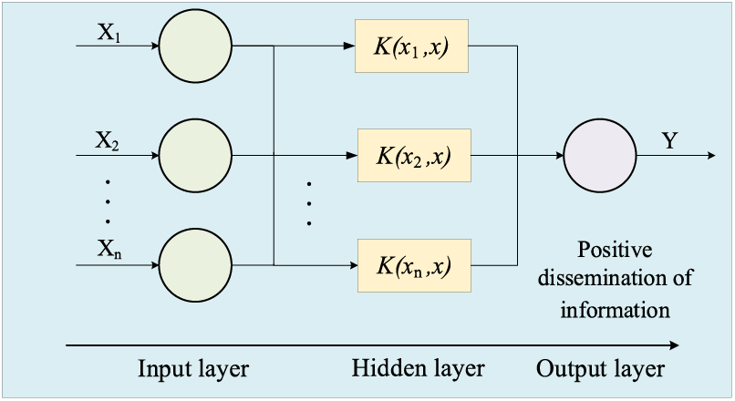
Figure 2: KELM model structure diagram

5.2 Model Evaluation Criteria

In order to more intuitively reflect the effectiveness of the proposed prediction method, the quantitative evaluation index of this experiment is calculated. By comparing the index calculation results of different power generation probability prediction methods, the mean error (ME), mean absolute error (MAE), root mean square error (RMSE), and R2 (determination coefficient) are used as the evaluation indexes of prediction. The calculation formulas are as follows [25]:

θME=1m∑i=1mYr−Y¯r(18)

θMAE=1m∑i=1m|Yr−Y^r|(19)

θRMSE=1m∑i=1m(Yr−Y^r)2(20)

R2=1−∑i=1m1m(Y^r−Yr¯)2∑i=1m1m(Yr−Yr¯)2(21)

where Yr is the photovoltaic power observation data; Y^r is the photovoltaic power prediction data; Yr¯ is the arithmetic mean of all photovoltaic power observation data; m is the sum of the predicted photovoltaic power points.

5.3 VMD-KELM Network Prediction Model

The schematic diagram of the prediction process proposed in this article is shown in Fig. 3. First, preprocess historical photovoltaic power data and meteorological data, information entropy is extracted, and various factors are analyzed that affect photovoltaic power efficiency. Conduct grey relational analysis on the factors, select typical meteorological elements, use the GMM algorithm to cluster these elements based on specific characteristics. The process is further refined to yield a more accurate and probable classification of meteorological results. Then, meteorological clusters under major extreme weather are selected to integrate their similar daily data, and the VMD-KELM network model is used to train the training set to obtain the trained network parameters and prediction errors. Finally, input the weather forecast data at the time to be predicted, predict the test set, and perform an error analysis on the results based on the model evaluation indicators to verify the accuracy and credibility of the results.

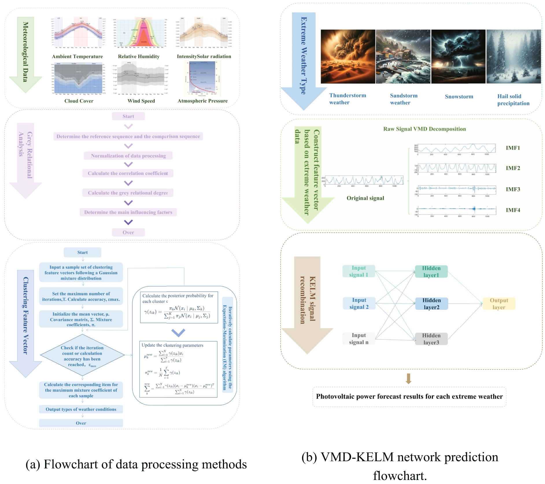
Figure 3: Flowchart of the forecasting method

6  Case Analysis

We set the maximum number of iterations for the clustering algorithm to 100, the initial learning rate to 0.01, the learning rate decay to 1.5, and the minimum learning rate to 10−4. The important parameters in the VMD-KELM network prediction model are shown in Table 3.

K represents the number of decomposed modes, that is, VMD decomposes the original signal into k sub-signals. α represents the penalty coefficient, which can control the smoothness during the decomposition process. τ is the noise tolerance and setting it to 0 means that the algorithm will try to reduce the reconstruction error as much as possible. DC (Direct Current) set to 0 means no DC component. Init represents the initial conditions that determine modal decomposition. Tol is the convergence tolerance. C represents the regularization coefficient, which is used to control the complexity of the model and avoid overfitting. γ is the parameter of the kernel function, which affects the width of the kernel function, thereby affecting the influence range of each data point in the feature space.

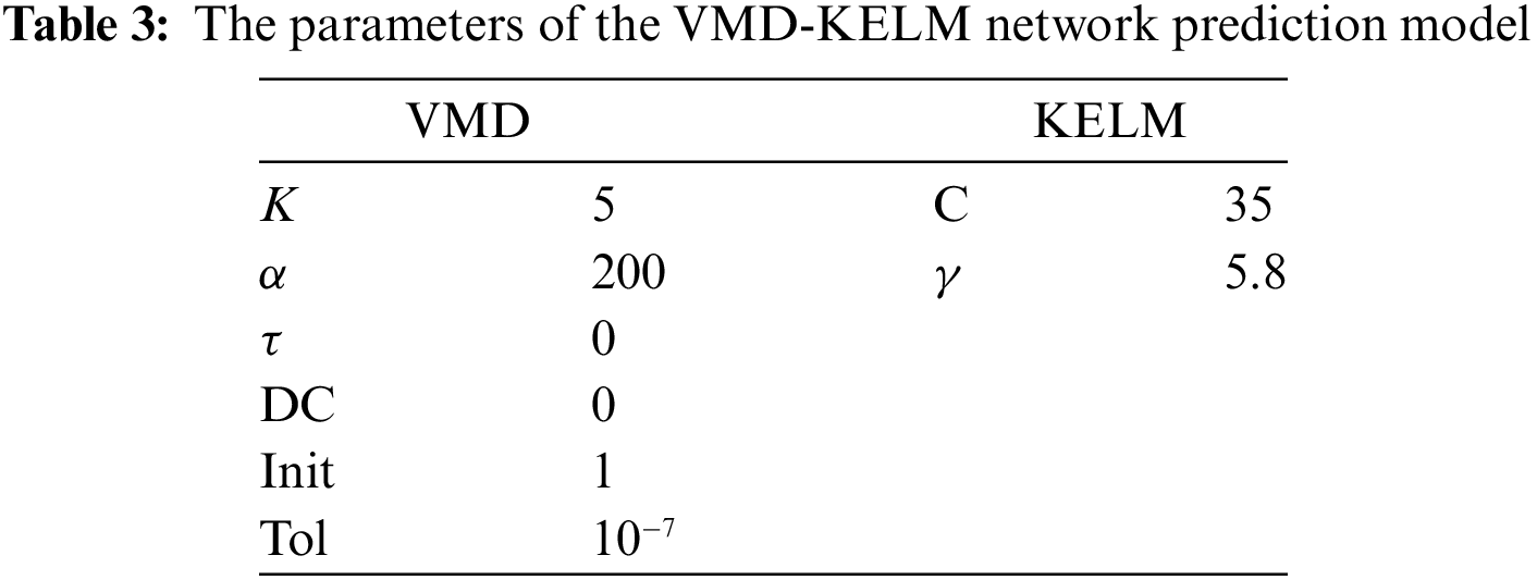
The values of each parameter were determined using K-fold cross-validation. The dataset was randomly divided into K subsets of equal size. During each iteration, one subset was designated as the test set while the remaining K − 1 subsets were used as the training set. This process was repeated K times, with a different subset chosen as the test set each time. This approach ensures the robustness and generalizability of the results.

Taking the photovoltaic power generation data of Nanjing City on 03 January 2023 as the test data, Fig. 4 shows the change histogram of the RMSE index calculated using the photovoltaic predicted value and the actual value under different parameter selections. The results help to validate the rationality of the selected parameters.

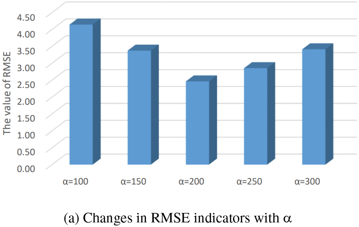
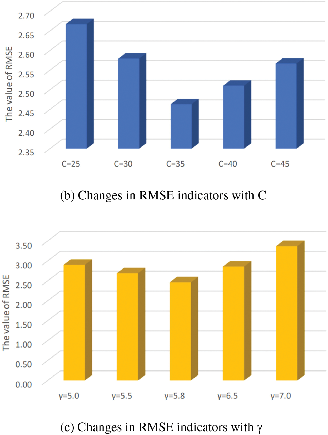
Figure 4: Changes in RMSE indicators for experimental results with different parameters

6.1 Comparison of Training and Prediction Effects of Various Network Models

In this section, we selected the photovoltaic power generation dataset of Nanjing, Jiangsu Province, China, for August 2023 for training and testing. The installed capacity of photovoltaic power generation in Nanjing is approximately 700 MW. The data includes all large ground-based photovoltaic power stations, commercial and industrial distributed photovoltaic power stations, and household photovoltaic power stations in Nanjing, with the values representing the sum of all these photovoltaic power stations.

This paper compares several typical photovoltaic power prediction network models with the VMD-KELM network model constructed in this paper, including the CNN-LSTM model and the QR (Quantile Regression)-BiLSTM network model. The selected dataset includes both training and testing sets, with 500 training samples and 215 testing samples. The time resolution of this dataset is 15 min, and only data with photovoltaic output power greater than 0 during the day is collected for training and testing. Each cycle lasts approximately 11–13 h, corresponding to a total of 44–52 data points. Inputs include environmental forecast data such as solar radiation, wind speed, ambient temperature, and cloud cover at the photovoltaic power stations, as well as power data for the corresponding times. The photovoltaic power prediction results and error evaluation of the training and testing sets are shown in Fig. 5, Tables 4, and 5 below.

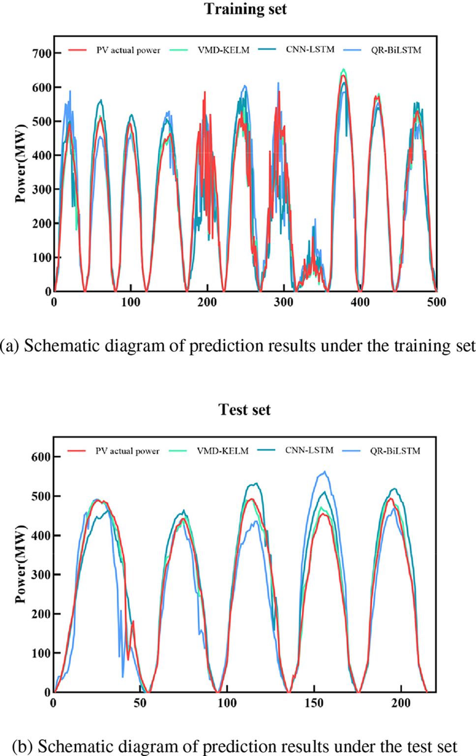
Figure 5: Schematic diagram of photovoltaic power prediction results by various forecasting network models

Fig. 5 illustrates that the QR-BiLSTM model predicts lower photovoltaic power when solar irradiance peaks, showing significant fluctuations and poor accuracy overall. On the other hand, the CNN-LSTM model predicts the trend more accurately but tends to overestimate values. In the training set, it is evident that significant changes in environmental factors lead to fluctuations in photovoltaic power, resulting in decreased accuracy across all three prediction methods during certain periods. However, the KELM model outperforms the other models by demonstrating greater resistance to interference and fluctuations, accurately predicting changing trends, and proving to be more suitable for photovoltaic power prediction under extreme weather conditions. Interestingly, the prediction accuracy of the three models is higher in the test set compared to the training set.

In the error-index evaluation, the R2 of the VMD-KELM network model is higher than that of the other two models, indicating that it better explains the variability of the dependent variable and produces more accurate prediction results. In contrast, the other two models have higher θME, θMAE, and θRMSE indices, indicating a significant decrease in prediction accuracy. Specifically, in the training set, the θMAE of the VMD-KELM model is 5.79% and 11.23% lower than that of the CNN-LSTM and QR-BiLSTM models, respectively. In the test set, these values are 8.40% and 15.67%, respectively. In addition, the θRMSE of the VMD-KELM model in the training set is 5.57% and 9.01% lower than that of the CNN-LSTM and QR-BiLSTM models, respectively. In the test set, these values are 8.67% and 12.57%, respectively. The data clearly show that the VMD-KELM model has higher prediction accuracy.

The VMD-KELM model has several significant advantages over other prediction models:

•   The VMD method is capable of effectively decomposing time series data, enabling a more accurate capture of the nonlinear and non-stationary characteristics present in the data. This ultimately enhances the accuracy of the overall forecasting model. KELM serves as an efficient learning mechanism that utilizes kernel techniques to process data, outperforming traditional linear models in handling nonlinear problems.

•   KELM utilizes a kernel method for input data processing. In comparison to conventional neural networks or linear regression models, KELM typically exhibits superior generalization abilities when encountering unfamiliar data. As a result, the VMD-KELM model can maintain high prediction accuracy while processing actual photovoltaic power generation data, even with limited data or significant changes in data characteristics.

•   VMD decomposition plays a crucial role in enabling the model to sustain high performance levels amidst significant input variability or interference. This method effectively separates noise from main signals, thereby improving the model’s resilience to environmental changes like cloud cover or sudden weather fluctuations.

6.2 Photovoltaic Power Prediction Results and Evaluation Indicators for Four Major Weather Conditions

After meteorological cluster classification, this article selects meteorological clusters under major weather from thunder types, precipitation weather types, fair-weather and cloud types, snowy types, and visual obstruction types, and selects thunderstorms, hail, solid precipitation, dust storms, and snowstorms, respectively. These are compared with data from clear sky day conditions (control group) to forecast photovoltaic power generation under five different weather types.

Due to the limited availability of historical weather and photovoltaic output data for major weather, the number of forecast data sets for these five major weather conditions is set to 144, and the time resolution is accurate to 5 min, that is, from 6:00 in the morning to 18:00 in the evening.

The experimental data are sourced from the photovoltaic power output dataset and meteorological data of Nanjing in 2023 and 2024. Weather data and PV actual power data for dust storm were collected on 11 April 2023, thunderstorms on 10 June 2023, snowstorms on 04 February 2024, and hail solid precipitation on 25 March 2023.

It can be concluded from Fig. 6 that the peak photovoltaic output power of the control group under clear day conditions is 476.35 kW. Under dust storms, thunderstorms, hail solid precipitation, and snowstorms, the peak photovoltaic output power decreases to 170.59 kW, 315.63 kW, 222.87 kW, and 327.90 kW, respectively, with the average output power reduced to 82.70 kW, 152.08 kW, 101.22 kW, and 132.92 kW, respectively. Compared to the photovoltaic output power on clear days, the average photovoltaic output power during the four major extreme weather events decreased by 68.84%, 42.70%, 61.86%, and 49.92%, respectively, showing a significant reduction in output during extreme weather. During dust storms, larger-sized sand and dust particles settle on the surface of photovoltaic panels, causing refraction, reflection, and scattering of surface radiation. This significantly impacts the power generation efficiency of photovoltaic power stations and leads to fluctuations in output. Additionally, dust storms can raise the temperature of photovoltaic modules, reducing their performance due to thermal attenuation of the cells.

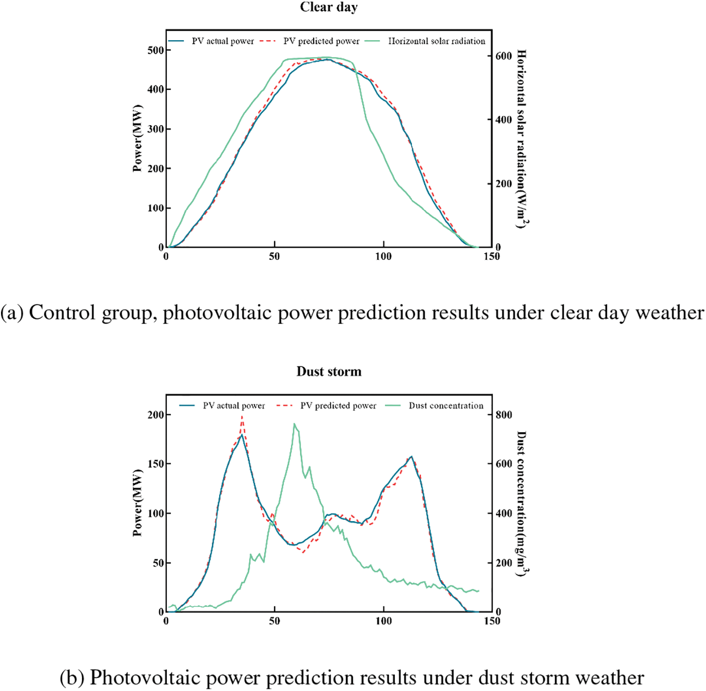
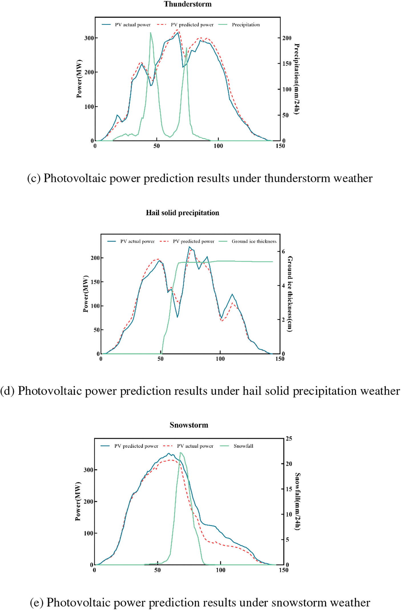
Figure 6: Photovoltaic power prediction results under different weather types

During snowstorm, snow accumulation on photovoltaic panels can obstruct sunlight, leading to a reduction in the solar radiation received. Additionally, the presence of snow on the panels hinders heat conduction from the air, reducing the panels' ability to generate heat. This diminishes the snow melting effect, further impacting the efficiency of photovoltaic power generation.

In hail and solid precipitation weather, the atmosphere contains a particularly thick unstable layer, and the water content in cumulonimbus clouds is extremely high, which greatly reduces the amount of solar radiation. Additionally, the formation of hail is generally accompanied by a rapid drop in temperature, which affects the temperature of photovoltaic modules and leads to a decrease in photovoltaic output power.

Thunderstorm weather and snowstorm weather have less impact on the output power of photovoltaic power stations compared to dust storms and hail solid precipitation. However, due to the weather characteristics, solar radiation is still lower than on sunny days, and the temperature is reduced, both of which have a certain effect on the actual output of photovoltaic power.

In Table 6, we can see the average predicted data and the average real data under five weather conditions, while Table 7 shows the different error indicators for each condition. From the comparative analysis of the data in both tables, it can be concluded that the prediction accuracy during snowstorm weather is worse than that of the other weather types. This is due to the limited accumulation of environmental factor data for snowstorm conditions, the difficulty in accurately predicting the snow thickness on photovoltaic panels, and the amount of snowfall in the area where the photovoltaic power station is located. As a result, the photovoltaic power prediction results are less accurate. Additionally, significant snow accumulation on the panels during snowstorms leads to the predicted value of photovoltaic power being higher than the actual value. In thunderstorm weather, the frequency and amplitude of solar radiation received by the photovoltaic panels are highly variable, and the trend of solar radiation is difficult to predict accurately. Therefore, the deviation in photovoltaic power prediction is relatively large for both thunderstorm and snowstorm conditions. In contrast, the photovoltaic power prediction under hail solid precipitation and dust storm conditions is more accurate. The order of prediction accuracy from highest to lowest is clear day, dust storm, hail solid precipitation, thunderstorm, and snowstorm.

7  Conclusions

In this paper, a photovoltaic power prediction model based on VMD-KELM under severe extreme weather is proposed. The main conclusions are as follows:

•   The meteorological factors of photovoltaic power generation are analyzed, and the GMM clustering algorithm can make the clustering results of meteorological data more accurate and reliable.

•   VMD is utilized to decompose the photovoltaic data into a series of intrinsic mode components with specific bandwidths, which effectively reduces the non-stationarity of the data. Subsequently, the data structure is reorganized using KELM to enhance the model’s prediction accuracy. By comparing this model’s performance with the CNN-LSTM and QR-BiLSTM networks, we have demonstrated that the VMD-KELM network used in this study offers superior predictive effectiveness.

•   Compared to normal clear day photovoltaic power generation, the average photovoltaic power generation under the four extreme weather conditions of dust storm thunderstorms, solid precipitation of hail, and snowstorm significantly decreases by 68.84%, 42.70%, 61.86%, 34.7%, and 49.92%, respectively.

•   The error-index analysis of photovoltaic power prediction under four kinds of major extreme weather shows that, according to its prediction accuracy, the prediction accuracy of photovoltaic power under dust storm weather is higher, while the prediction accuracy of photovoltaic power under snowstorm weather is the lowest. The order of prediction accuracy from high to low is clear day, dust storm, solid hail precipitation, thunderstorm, and snowstorm.

The limitations of the study in this paper are as follows:

This study is limited by the absence of prior research in the field. While most studies on photovoltaic power prediction focus on normal weather conditions, this article explores the impact of extreme weather conditions on meteorological data, which can fluctuate significantly and pose challenges for the accurate prediction of photovoltaic power. Additionally, the lack of extreme weather data in the same area results in an insufficient training volume for the prediction model, ultimately affecting the accuracy of the predictions. Furthermore, it is important to consider that different types of extreme weather may require specific prediction methods, and the universal method applied in this article may not necessarily be the optimal model for all scenarios.

Acknowledgement: The authors would like to express their sincere gratitude to China Electric Power Research Institute (National Key Laboratory of Renewable Energy Grid Integration) for providing financial support for the research contents of this paper.

Funding Statement: This research was funded by the Open Fund of National Key Laboratory of Renewable Energy Grid Integration (China Electric Power Research Institute) (No. NYB51202301624).

Author Contributions: The authors confirm contribution to the paper as follows: study conception and design: Yuxuan Zhao; analysis and interpretation of results: Wenjun Xu; supervision: Bo Wang and Shu Wang; software: Gang Ma. All authors reviewed the results and approved the final version of the manuscript.

Availability of Data and Materials: Data from the study results are available on request from the corresponding author, Yuxuan Zhao.

Ethics Approval: Not applicable.

Conflicts of Interest: The authors declare that they have no conflicts of interest to report regarding the present study.

References

1. IEA, “Paris,” Licence: CC BY 4.0. Renewables 2023–Analysis-IEA. Accessed: Sep. 2, 2024. [Online]. Available: https://www.iea.org/reports/renewables-2023 [Google Scholar]

2. S. S. Dipta et al., “Highly efficient double-side-passivated perovskite solar cells for reduced degradation and low photovoltage loss,” Sol. Energy Mater. Sol. Cells, vol. 266, 2024, Art. no. 112655. doi: 10.1016/j.solmat.2023.112655. [Google Scholar] [CrossRef]

3. S. C. Johnson, D. J. Papageorgiou, D. S. Mallapragada, T. A. Deetjen, J. D. Rhodes and M. E. Webber, “Evaluating rotational inertia as a component of grid reliability with high penetrations of variable renewable energy,” Energy, vol. 180, pp. 258–271, 2019. doi: 10.1016/j.energy.2019.04.216. [Google Scholar] [CrossRef]

4. C. Ma, R. Han, Z. An, T. Hu, and M. Jin, “Weather-driven solar power forecasting using D-informer: Enhancing predictions with climate variables,” Energy Eng., vol. 121, no. 5, pp. 1245–1261, 2024. doi: 10.32604/ee.2024.046644. [Google Scholar] [CrossRef]

5. C. Deline et al., “Performance index assessment for the PV fleet performance data initiative,” in 2021 IEEE 48th Photovoltaic Specialists Conf. (PVSC), 2021, pp. 1486–1491. doi: 10.1109/pvsc43889.2021.9518760. [Google Scholar] [CrossRef]

6. D. C. Jordan, K. Perry, R. White, and C. Deline, “Extreme weather and PV performance,” IEEE J. Photovolt., vol. 13, no. 6, pp. 830–835, 2023. doi: 10.1109/JPHOTOV.2023.3304357. [Google Scholar] [CrossRef]

7. I. Yury and A. Martirosyan, “The development of the soderberg electrolyzer electromagnetic field’s state monitoring system,” Sci. Rep., vol. 14, no. 1, Feb. 12, 2024, Art. no. 3501. doi: 10.1038/s41598-024-52002-w. [Google Scholar] [PubMed] [CrossRef]

8. N. Saxena et al., “Hybrid KNN-SVM machine learning approach for solar power forecasting,” Environ. Chall., vol. 14, 2024, Art. no. 100838. doi: 10.1016/j.envc.2024.100838. [Google Scholar] [CrossRef]

9. A. Kazemi, R. Boostani, M. Odeh, and M. R. Al-Mousa, “Two-layer SVM, towards deep statistical learning,” in 2022 Int. Eng. Conf. Electr., Energy, Artif. Intell. (EICEEAI), 2022, pp. 1–6. doi: 10.1109/eiceeai56378.2022.10050469. [Google Scholar] [CrossRef]

10. C. Hajjaj et al., “Comparing photovoltaic power prediction: Ground-based measurements vs. satellite data using an ANN model,” IEEE J. Photovolt., vol. 13, no. 6, pp. 998–1006, 2023. doi: 10.1109/JPHOTOV.2023.3306827. [Google Scholar] [CrossRef]

11. Z. Hu, Y. Gao, S. Ji, M. Mae, and T. Imaizumi, “Improved multistep ahead photovoltaic power prediction model based on LSTM and self-attention with weather forecast data,” Appl. Energy, vol. 359, 2024. doi: 10.1016/j.apenergy.2024.122709. [Google Scholar] [CrossRef]

12. D. K. Dhaked, S. Dadhich, and D. Birla, “Power output forecasting of solar photovoltaic plant using LSTM,” Green Energy Intell. Transp., vol. 2, no. 5, 2023. doi: 10.1016/j.geits.2023.100113. [Google Scholar] [CrossRef]

13. F. Zhang, X. Ren, and Y. Liu, “A refined wind power forecasting method with high temporal resolution based on light convolutional neural network architecture,” Energies, vol. 17, no. 5, 2024, Art. no. 1183. doi: 10.3390/en17051183. [Google Scholar] [CrossRef]

14. A. Jakoplić, D. Franković, J. Havelka, and H. Bulat, “Short-term photovoltaic power plant output forecasting using sky images and deep learning,” Energies, vol. 16, no. 14, 2023, Art. no. 5428. doi: 10.3390/en16145428. [Google Scholar] [CrossRef]

15. A. Zendehboudi, M. A. Baseer, and R. Saidur, “Application of support vector machine models for forecasting solar and wind energy resources: A review,” J. Clean. Prod., vol. 199, pp. 272–285, 2018. doi: 10.1016/j.jclepro.2018.07.164. [Google Scholar] [CrossRef]

16. N. Li et al., “Research on short-term photovoltaic power prediction based on multi-scale similar days and ESN-KELM dual core prediction model,” Energy, vol. 277, 2023, Art. no. 127557. doi: 10.1016/j.energy.2023.127557. [Google Scholar] [CrossRef]

17. T. Limouni, R. Yaagoubi, K. Bouziane, K. Guissi, and E. H. Baali, “Accurate one step and multistep forecasting of very short-term PV power using LSTM-TCN model,” Renew. Energy, vol. 205, pp. 1010–1024, 2023. doi: 10.1016/j.renene.2023.01.118. [Google Scholar] [CrossRef]

18. Q. Li, X. Zhang, T. Ma, D. Liu, H. Wang and W. Hu, “A multi-step ahead photovoltaic power forecasting model based on TimeGAN, Soft DTW-based K-medoids clustering, and a CNN-GRU hybrid neural network,” Energy Rep., vol. 8, pp. 10346–10362, 2022. doi: 10.1016/j.egyr.2022.08.180. [Google Scholar] [CrossRef]

19. F. Nicoletti and P. Bevilacqua, “Hourly photovoltaic production prediction using numerical weather data and neural networks for solar energy decision support,” Energies, vol. 17, no. 2, 2024, Art. no. 466. doi: 10.3390/en17020466. [Google Scholar] [CrossRef]

20. J. Dai, Y. Xiang, and Q. Tang, “A correlation-XGBoost based distributed photovoltaic output prediction method considering regional meteorological factor,” in 2023 IEEE/IAS Ind. Commer. Power Syst. Asia (I&CPS Asia), 2023, pp. 2052–2056. doi: 10.1109/ICPSAsia58343.2023.10294804. [Google Scholar] [CrossRef]

21. T. Wu et al., “Combined IXGBoost-KELM short-term photovoltaic power prediction model based on multidimensional similar day clustering and dual decomposition,” Energy, vol. 288, 2024, Art. no. 129770. doi: 10.1016/j.energy.2023.129770. [Google Scholar] [CrossRef]

22. W. Lin, B. Zhang, H. Li, and R. Lu, “Multi-step prediction of photovoltaic power based on two-stage decomposition and BILSTM,” Neurocomputing, vol. 504, pp. 56–67, 2022. doi: 10.1016/j.neucom.2022.06.117. [Google Scholar] [CrossRef]

23. J. P. Wang, Z. Yang, G. Xin, G. Jeremy, and Z. Xin, “A hybrid predicting model for the daily photovoltaic output based on fuzzy clustering of meteorological data and joint algorithm of GAPS and RBF neural network,” IEEE Access, vol. 10, pp. 30005–30017, 2022. doi: 10.1109/ACCESS.2022.3159655. [Google Scholar] [CrossRef]

24. J. Thaker, R. Höller, and M. Kapasi, “Short-term solar irradiance prediction with a hybrid ensemble model using EUMETSAT satellite images,” Energies, vol. 17, no. 2, 2024, Art. no. 329. doi: 10.3390/en17020329. [Google Scholar] [CrossRef]

25. R. Blaga, A. Sabadus, N. Stefu, C. Dughir, M. Paulescu and V. Badescu, “A current perspective on the accuracy of incoming solar energy forecasting,” Prog. Energy Combust. Sci., vol. 70, pp. 119–144, 2019. doi: 10.1016/j.pecs.2018.10.003. [Google Scholar] [CrossRef]