Multi-Lever Early Warning for Wind and Photovoltaic Power Ramp Events Based on Neural Network and Fuzzy Logic

Nomenclature

1  Introduction

In recent years, with the transformation of the energy structure and the rapid development of renewable generation, renewable energy power ramp events (REPREs) have become a significant challenge in the power system [1]. Renewable energy exhibits volatility and intermittency, leading to drastic changes in output power within short periods under extreme weather conditions, the change process referred to as a power ramp event. Especially in down-ramp events, the rapid loss of active power support in power system significantly undermines the power balance and stability of the grid [2,3]. Improper handling of power ramp events can easily result in accidents and severe chain reactions, posing a serious threat to the secure and stable operation of the power system [4]. Therefore, early warning for REPRE is crucial for maintaining the active power balance of the power system.

Early warning is a system or process that provides information before the occurrence of disasters. The effectiveness of an early warning system depends on the accuracy of predictions and the reasonableness of warning indicators [5]. Early warning methodologies are primarily divided into statistical methods and physical analysis methods. Statistical methods depend on historical data and probabilistic models to forecast future events. In contrast, physical methods mainly rely on monitoring and analyzing the physical parameters of the system to predict potential hazardous situations, utilizing the inherent characteristics and potential principles of the system. Given that REPREs are low-probability events, there is often insufficient data to support statistical methods, making physical analysis methods more suitable for warning of power ramp events [6]. To establish a database for accurate power time series data, an on-time single-phase power smart meter is proposed in [7] for collecting generation/load profiles in PV household-prosumer facilities. However, this household meter is not suitable for large-scale renewable energy power generation monitoring. Currently, energy management systems remain the optimal choice for acquiring power data from power grid nodes.

Early warning indicators are a crucial component of early warning system. Currently, power ramp event detection relies primarily on calculating characteristic values such as ramp amplitude and ramp rate, comparing them with preset thresholds, and then determining whether changes in renewable generation over a period of time constitute a power ramp event [8–10]. However, these preset thresholds are only applicable to specific generation station and operating condition. Different power systems or different operational states of the same power system have varying tolerances for renewable power fluctuations. Therefore, a uniform standard for identifying power ramp events is infeasible. In addition to analyzing the power ramp process, it is essential to consider the operating conditions and power fluctuation tolerance of power system when generating early warning results. Power imbalance caused by power ramp events in the power system can generally be attributed to two primary reasons: (1) the rate of power change surpasses the regulation speed of power system; (2) the amplitude of power change exceeds the reserve capacity of power system [11,12]. The former is usually more critical, necessitating an analysis of both the regulation capacity and regulation speed of power system. In [13], power ramp events are identified from the perspective of ramp rate, considering various power control measures, but no system operational risk indicators are provided. In [14,15], a predetermined severity function is employed to classify risk levels. In [16], the amount of load to be removed to ensure system safety is used as a risk classification metric. However, these methods fail to deeply analyze the operating status of power control measures and cannot effectively guide the subsequent prevention and control decisions. In [10], the warning boundaries are divided based on the interval analysis by calculating the power regulation capacity of different thermal power units, providing an early warning system for wind power ramp process. However, this method only calculates the power control capability of thermal power units and cannot fully reflect the power control capability of the power system. The energy storage system (ESS) has the characteristic of fast response, which can improve the flexibility and controllability of the power grid [17]. Furthermore, the grid-PV-ESS integrated system can enhance the resilience of the power supply system for residential electricity users [18]. During power ramp process, power control methods incorporating ESS can better maintain the balance between generation and load [19], while also reducing operational costs [20]. Additionally, different regional power grids are interconnected via tie lines [21], ensuring the stable operation of the entire power grid through power complementarity [22]. Therefore, it is necessary to consider the power regulation ability of the internal and external power grid, analyze the ability to withstand the power ramp process of power system, and develop appropriate early warning indicators.

To address the above problems, this paper proposes an early warning method for REPREs based on long short-term memory (LSTM) network and fuzzy rules. First, the energy management strategy (EMS) emphasizes the need for power system to reduce energy production costs while ensuring continuous load supply [23]. Similarly, low-cost control scheme should be prioritized when solving REPREs. A REPRE warning level ranking strategy based on control cost is proposed to determine the dispatch order of power control measures. Second, the LSTM network demonstrates superior performance in processing power time series data [24–26]. A power prediction model for tie lines is established based on the LSTM network, determining the power support capacity of the external grid. Finally, the concept of net load is introduced to represent the power deficit of power grid, and an early warning system is established based on fuzzy rules [27,28]. The classification boundaries are processed using fuzzy logic to reflect the risk attitudes of dispatchers and to mitigate the impact of power prediction errors.

The contributions of this paper are threefold. (1) Proposing an early warning level ranking strategy for REPREs based on control costs, which effectively guides warning calculation and preventive control decision-making. The proposed ranking strategy considers the power support capabilities of ESS and external grids, rather than being limited to thermal power generation. (2) Developing a power prediction model for tie lines using the LSTM network, which enhances the accuracy of assessing the power support capacity of external grids. On this basis, the tolerance to REPREs of power system can be dynamically evaluated, allowing for the identification of power ramp events rather than relying on fixed thresholds. (3) Proposing an early warning method for REPREs based on fuzzy rules, which effectively addresses the issue of warning boundary value attribution. This method allows dispatchers to adjust the warning strategy according to their risk attitudes, reduces the impact of prediction errors, and develops effective prevention and control strategy.

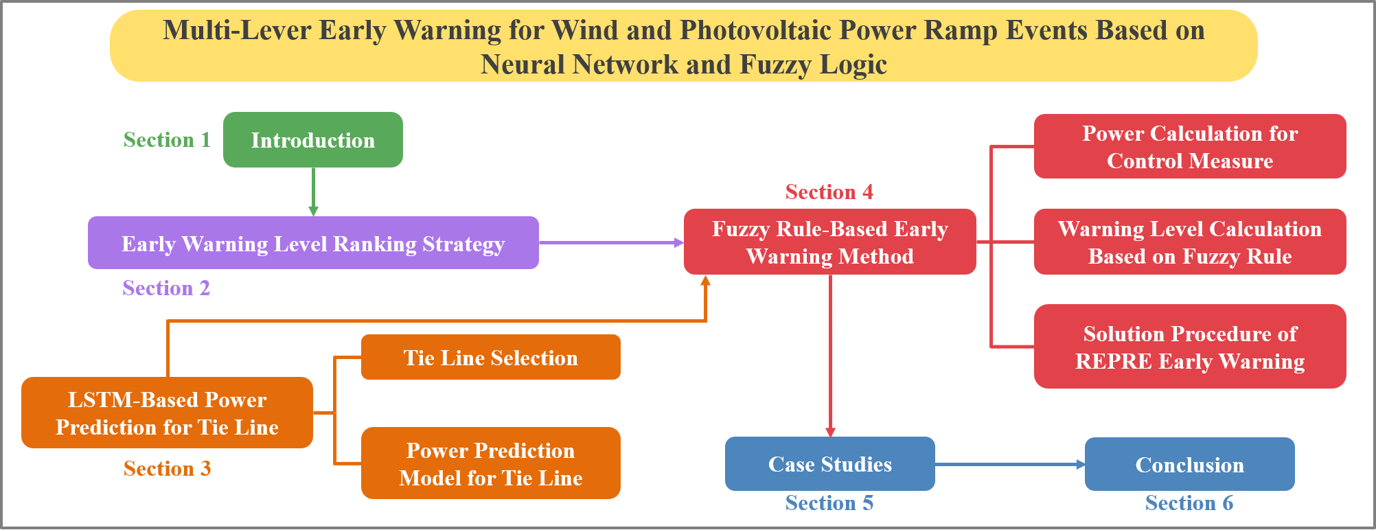
The remainder of this paper is organized as follows. The early warning level ranking strategy is introduced in Section 2. The prediction model for tie lines based on LSTM network is constructed in Section 3. The early warning method and solution procedure of REPREs are shown in Section 4. Case study is presented in Section 5. Finally, Section 6 draws conclusions.

2  Early Warning Level Ranking Strategy

The system ability to cope with the volatility of renewable energy generation becomes a critical issue in power system operation [29]. Under the influence of extreme weather, the power output of renewable energy power plants decreases rapidly, disrupting the active power balance of power grid. To address this issue, appropriate regulatory strategies need to be developed. The operating costs associated with different power control measures are distinct. Low-cost control measures should be prioritized while ensuring the secure and stable operation of the power system. However, when the active power deficit in the grid is significant, higher-cost control measures must be employed [30]. Therefore, the higher the control costs of the control measures adopted to ensure the safe operation of power system, the greater the active power deficit in the power gird, and the higher the corresponding risk level.

From the perspective of regional grid, power control measures are categorized into intra-area and inter-area control measures. In this paper, intra-area control measures include conventional thermal generation, independent energy storage system, and load management; only the power dispatch of tie lines is considered the inter-area control measure. Conventional thermal generation control measures can be divided into automatic generation control (AGC) and thermal generation dispatch [31]. The power output of thermal power units can be adjusted by AGC without requiring manual adjustments to the power dispatch plan of grid, resulting in the lowest control costs. In contrast, the thermal generation dispatch requires operators to adjust scheduling plans, potentially involving unit start-up issues, meaning higher control costs. Due to its quick response capability and independence from coal consumption [32], the independent energy storage system has significant advantages in dealing with power ramp events compared to the thermal generation dispatch. Therefore, the ESS should be given scheduling priority.

In general, the power transmission plan between regional power grids is not affected by active power adjustments within a regional grid. However, tie line power adjustments alter the power transmission plan, incurring additional control costs [33]. Therefore, compared to intra-regional dispatch control measures, the control costs of tie line power dispatch are higher. In contrast to the aforementioned preventive control measures, load management may affect the normal power supply to users. When other control measures fail to maintain the active power balance of the power grid, load shedding is implemented according to contingency plans to prevent frequency instability [34], resulting in significant economic losses [35]. Therefore, load shedding is the most costly power control measure.

Based on the above analysis, the warning levels are divided into five levels in ascending order of risk, as shown in Fig. 1. Level 0 corresponds to AGC and indicates that the power system is in a secure operating condition. Levels I to III indicate that the power system is insecure and appropriate preventive control measures need to be taken. Level IV indicates that the power system is in an extremely dangerous state with frequency instability and that emergency control measures are needed. The warning levels reflect the secure status of power system during changes in renewable energy output. In addition to guiding the formulation of preventive control strategies, the warning results presented in this paper also warn of potential power outages due to power ramp events.

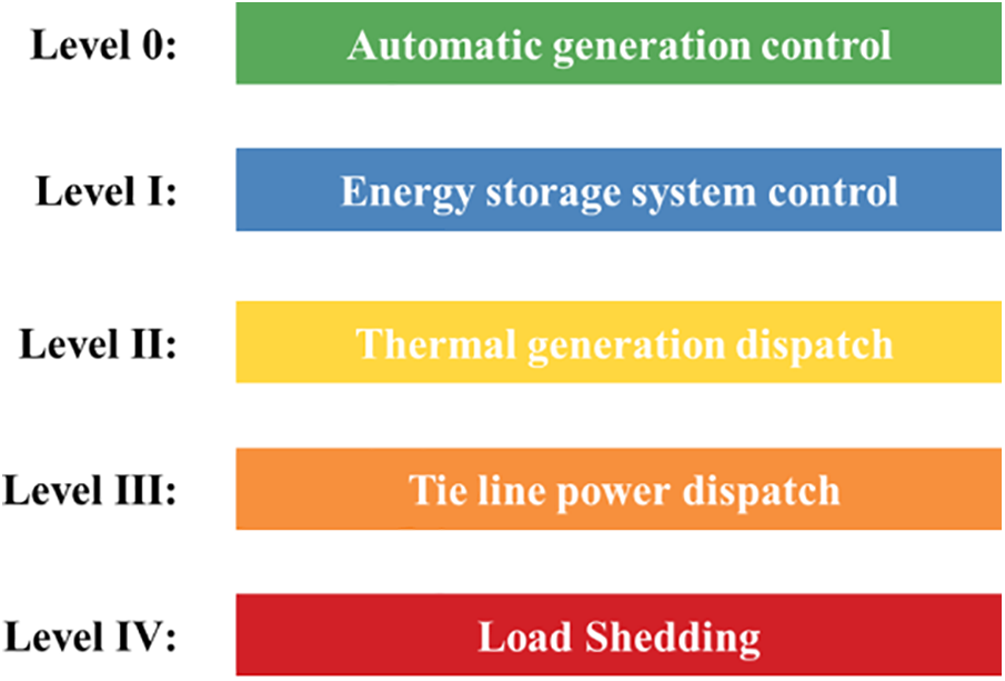
Figure 1: Schematic diagram of early warning grading

3  LSTM-Based Power Prediction for Tie Line

For regional grids, the operating status of local power control measures can be directly obtained, allowing for the analysis of adjustable power over the next four hours. However, the adjustable power of tie lines is subject to dynamic changes, constrained by the operating status and spare capacity of the external grid [36]. Therefore, calculating the adjustable power for the next four hours based on the current transmission power is infeasible. To address this issue, this section establishes a power prediction model for tie lines using an LSTM network. The power flow of tie lines over the next four hours during regular operation is predicted by the prediction model. Then, the adjustable power of tie lines for the next four hours can be calculated based on the total transfer capability and power regulation speed of tie lines.

3.1 Tie Line Selection

When power within the regional grid changes, only a portion of tie lines power experience significant variations. To simplify the calculation process, the tie lines with sensitivities exceeding a predetermined threshold are selected out by calculating the sensitivity of each tie line to the power changes within the regional grid. The tie lines with high sensitivity are then used as prediction targets. The formula to calculate the sensitivity of the i-th tie line is as follows:

β(i)=|Pline(i)−Pline_0(i)|Pline_abs×100%(1)

where Pline_0 and Pline denote the transmission power of the i-th tie line before and after the power adjustment within the grid, respectively; and Pline_abs denotes the sum of the absolute values of the transmission power changes of all tie lines.

Based on the current calculation results, the sensitivity of each tie line is obtained. A suitable threshold is set to screen out the effective tie lines.

3.2 Power Prediction Model for Tie Line

During normal grid operation, data for tie line power, load power, and the output of various power generation stations is typically updated every 15 min. Over time, this generates a series of continuous data with complex intrinsic relationships in the time dimension. To accurately predict the power of the tie lines based on known power time series data, it is essential to fully explore the inherent correlations between these time series data. The LSTM network is particularly effective in capturing the inherent correlations in time series data, offering significant advantages in forecasting such data.

3.2.1 LSTM Network

The LSTM network is a specialized type of recurrent neural network that incorporates memory units capable of retaining useful input data information over extended periods. The primary components of the LSTM network include the forget gate, input gate, output gate, and cell state. The detailed structure of the LSTM unit is illustrated in Fig. 2, and the equations for each variable are as follows:

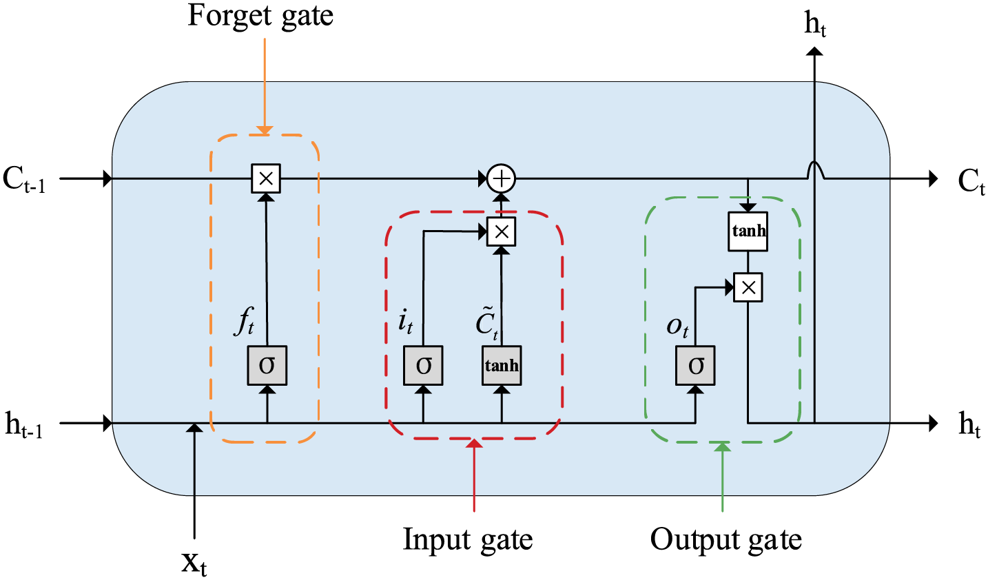
Figure 2: Structure of LSTM unit

ft=σ(Wf⋅[ht−1, xt]+bf)(2)

it=σ(Wi⋅[ht−1, xt]+bi)(3)

C∼t=tanh⁡(Wc⋅[ht−1, xt]+bc)(4)

ot=σ(Wo⋅[ht−1, xt]+bo)(5)

Ct=ft⊗Ct−1+it⊗C∼t(6)

ht=ot⊗tanh⁡(Ct)(7)

From the above equations, ft denotes the output of the forget gate; it and C∼t denote the variables in the input gate; ot denotes the output of the output gate; ht−1 and ht denote the outputs at moments t−1 and t; ht−1 and xt comprise the inputs at moment t; Ct−1 and Ct denote the variables of the memory cells at moments t−1 and t; Wf, Wi, Wc, Wo are the weight matrices of the input variables of the corresponding gates; bf, bi, bc, bo are the bias entries in the corresponding gates; σ denotes the sigmoid function.

3.2.2 Procedure of Power Prediction

The accuracy of the prediction model tends to decrease as the prediction timescale increases. To mitigate this issue, an optimized method for prediction results is proposed. As shown in Fig. 3, four distinct prediction models are constructed with different prediction scales ranging from 15 min to 4 h, using data intervals of 15 min. The optimal prediction results from each model are then integrated to derive the final 4-h tie line power prediction, significantly enhancing the accuracy of the 4-h prediction model.

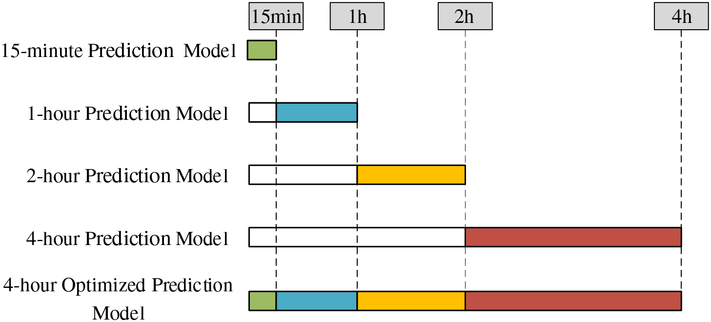
Figure 3: Schematic diagram of the model optimization process

The first step in constructing the prediction model based on the LSTM network is determining its input and output sequences. Due to the large number of nodes in the regional power grid, using the original node data as model input would be time-consuming. To address this issue, the overall power of the renewable energy cluster is utilized as a single feature, thus simplifying the network structure and enhancing computational efficiency. The input data features include the historical power of load, each renewable energy cluster, and each tie line. The output data features are the power of selected tie lines.

After determining the input and output data, the original data are normalized to the [0, 1] interval. This normalization process eliminates the influence of different scales, accelerates model training speed, and facilitates faster model convergence. The normalization formula is as follows:

x^i=xi−xminxmax−xmin(8)

where xi and x^i denote the values before and after normalization; xmax and xmin denote the maximum and minimum values of the feature x.

Finally, the network parameters for each prediction model are established. All prediction models employ a two-layer LSTM structure, with parameters such as input time series length and the number of hidden layers adjusted based on the prediction timescale. The predicted values for each model are obtained after denormalizing the output of the fully connected layer. Then, the predicted values for the tie line transmission power over four hours (16 time points) are derived by combining the outputs of these models.

4  Fuzzy Rule-Based Early Warning Method

4.1 Power Calculation for Control Measure

The impact of REPREs on the power system is primarily manifested in the ramp rate and ramp amplitude, necessitating that power control measures provide the corresponding regulation speed and capacity [37]. Given the high uncertainty inherent in renewable energy generation, it is crucial to quantitatively analyze the dynamic regulation capability of power control measures. In this section, the adjustable power of each power control measure is calculated at 15-min intervals to effectively evaluate the ability of power system to manage power fluctuations across various time scales. Based on the proposed risk ranking strategy, the controllable power interval of each power control measure for each period is calculated sequentially.

4.1.1 Automatic Generation Control

When the power system experiences moderate fluctuations, AGC effectively mitigates these disturbances and restores the system frequency to its nominal value [38]. AGC consists of two principal components: primary frequency control (PFC) and secondary frequency control (SFC). PFC serves as the fundamental automatic frequency regulation in the power system but typically results in a steady-state frequency deviation. SFC, generally implemented subsequent to PFC, corrects the residual frequency deviation remaining after PFC has been applied. Therefore, to the maintain the system frequency at the standard value in each time interval, the maximum adjustable power of the SFC is used as the maximum adjustable power of the AGC. The formulas for determining the adjustable power of SFC in each time interval are as follows:

ΔPAGC_j(i)={PAGC_max(i)−PAGC_j(i),PAGC_max(i)−PAGC_j(i)<RAGC(i)×ΔtRAGC(i)×Δt,PAGC_max(i)−PAGC_j(i)≥RAGC(i)×Δt(9)

PSFC(j)=∑i=1NAGCΔPAGC_j(i)−(NGR+D)×Δf(10)

From the above equations, ΔPAGC_j(i) denotes the maximum adjustable power of the i-th AGC unit in period j; PAGC_max(i) and PAGC_j(i) denote the upper limit and initial power of the i-th AGC unit in period j, respectively; RAGC(i) denotes the maximum ramp rate of the i-th AGC unit; Δt denotes the time interval (i.e., 15 min); PSFC(j) denotes the maximum adjustable power of the SFC in period j; NG and NAGC denote the total number of units and the number of AGC units, respectively; R denotes the unit survey rate; D denotes the load-damping constant; Δf denotes the static frequency deviation. Therefore, the adjustable power of the SFC primarily depends on the adjustable power of AGC units, which is limited by the number of AGC units and their operation status.

4.1.2 Energy Storage System Control

ESS can release or absorb power as needed and respond within milliseconds for rapid power regulation. In this study, the independent energy storage system is used as the calculation subject, and the adjustable power of the ESS in each time interval is calculated as follows:

PESS(j)={SOCj×PN,SOCj≤Pdis_max×ΔtPNPdis_max×Δt,SOCj>Pdis_max×ΔtPN(11)

where PESS(j) denotes the maximum adjustable power of the ESS in period j; SOCj denotes the state of charge in period j; PN denotes the rated capacity; Pdis_max denotes the maximum discharge power. Therefore, the adjustable power of the ESS depends on its state of charge (SOC) and discharge power.

4.1.3 Thermal Generation Dispatch

Conventional thermal power reverse units are mainly divided into two categories: spinning reserve units and non-spinning reserve units [30]. Spinning reserve units are online units operating below full load that can quickly respond to system demand, whereas non-spinning reserve units are offline units that can be activated when needed, but this process takes longer and cannot provide an immediate response. Given the characteristics of the two types of units, the formula for calculating the power adjustability is as follows:

ΔPSr_j(i)={PSr_max(i)−PSr_j(i),PSr_max(i)−PSr_j(i)<RSr(i)×ΔtRSr(i)×Δt,PSr_max(i)−PSr_j(i)≥RSr(i)×Δt(12)

ΔPNSr_j(k)={0,t<tst(k)PNSr_max(k)−PNSr_j(k),t≥tst(k)&PNSr_max(k)−PNSr_j(k)<RNSr(k)×ΔtRNSr_j(k)×Δt,t≥tst(k)&PNSr_max(k)−PNSr_j(k)≥RNSr(k)×Δt(13)

PTGD(j)=∑i=1NSrΔPSr_j(i)+∑k=1NNSrΔPNSr_j(k)−(NGR+D)×Δf(14)

From the above equations, ΔPSr_j(i), ΔPNSr_j(k) denote the adjustable power of the i-th spinning reserve unit and the k-th non-spinning reserve unit in period j, respectively; PSr_max(i), PNSr_max(k) denote the upper limit power of the i-th spinning reserve unit and the k-th non-spinning reserve unit; PSr_j(i), PNSr_j(k) denote the initial power of the i-th spinning reserve unit and the k-th non-spinning reserve unit in period j; RSr(i), RNSr(k) denote the maximum ramping rate of the i-th spinning reserve unit and the k-th non-spinning reserve unit; t, tst(k) denote the initial time of the period j and the start-up time of the k-th non-spinning reserve unit; PTGD(j) denotes the maximum adjustable power of thermal power units under dispatch control in j-th period; NSr, NNSr denote the total number of spinning and non-spinning reserve units.

Therefore, in the dispatching process of conventional thermal power units, the adjustable power is mainly influenced by the number of units, the ramp rate, and the start-up time of the non-spinning reserve units.

4.1.4 Tie Line Power Dispatch

Tie lines play a crucial role in balancing load fluctuations, responding to emergencies, and enhancing power system stability and reliability. During the REPREs, it may be necessary to adjust the power transmission of tie lines between different regional power grids for power dispatch. However, the adjustable power of tie lines is constrained by factors such as total transfer capability, power flow change rate, economics, and market contracts. Given that power ramp events prioritize the security of power system, this paper considers only the limitations of total transfer capability and power ramp rate. The related calculation formulas are as follows:

ΔPline_j(i)={Pline_max(i)−Pline_j(i),Pline_max(i)−Pline_j(i)<Rline(i)×ΔtRline(i)×Δt,Pline_max(i)−Pline_j(i)≥Rline(i)×Δt(15)

PTie−line(j)=∑i=1NlineΔPline_j(i)(16)

From the above equations, ΔPline_j(i) denotes the adjustable power of the i-th tie line in period j; Pline_max(i), Rline(i) denote the upper limit of power transmission and ramp rate of the i-th tie line, respectively; Pline_j(i) denotes the initial power of the i-th tie line in period j; PTie−line(j) denotes the total maximum adjustable power of the tie line in period j; and Nline denotes the total number of tie lines.

In summary, the adjustable power of each power control measure depends on the operating state at the beginning of each period. Changes in the operating state are influenced by the power deficit of power grid during the corresponding period. In this paper, the net load change ΔPnet is used to represent the power demand for each period. If the power deficit from the previous period is not fully compensated, the remaining power deficit needs to be added to the current period. The power adjustments of different control measures in the same period are calculated sequentially according to the risk ranking strategy to determine the course of action. The relevant formulas for ΔPnet are as follows:

Pnet(j)=Pload(j)−Ppv(j)−Pwind(j)(17)

ΔPnet(j)=Pnet(j)−Pnet(j−1)(18)

ΔPnet(j+1)={ΔPnet(j+1),ΔPnet(j)≤Pcontrol(j)ΔPnet(j+1)+ΔPnet(j)−Pcontrol(j),ΔPnet(j)>Pcontrol(j)(19)

From the above equations, Pnet(j), Pload(j), Ppv(j), Pwind(j) are the net load, load, photovoltaic power, and wind power at time j, respectively; and Pcontrol(j) denotes the maximum adjustable power of all power control measures in period j.

Taking the AGC and ESS as an example, the power ΔPess(j) to be smoothed by the ESS in period j is calculated as follows:

ΔPess(j)={0,ΔPnet(j)≤PSFC(j)ΔPnet(j)−PSFC(j),ΔPnet(j)>PSFC(j)(20)

Specifically, if the AGC can effectively smooth out power fluctuations, the ESS remains inactive. Conversely, when the AGC is unable to fully compensate for the fluctuations, the ESS is required to mitigate the residual power.

4.2 Warning Level Calculation Based on Fuzzy Rule

4.2.1 Classification Problem of Warning Boundary Values

Based on the calculation method for adjustable power and power deficit proposed in Section 4.1, the power deficit for each period is compared with the adjustable power interval of control measures to establish a relative relationship. Subsequently, the warning level is classified according to the risk ranking strategy. Fig. 4 illustrates a scenario where the power deficit ΔPnet is at the junction of different adjustable power intervals. In such cases, the opinions of dispatcher may diverge: some may adopt a conservative stance and classify the danger level as Level II, while others may assess it as Level I.

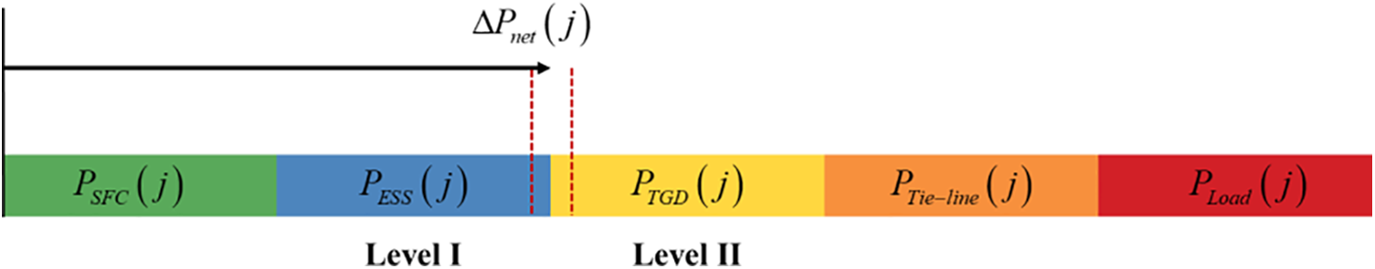
Figure 4: Schematic diagram of the risk attitude

To resolve this discrepancy, this paper proposes a warning grading method based on fuzzy rules. The warning levels are determined by employing the membership function and the principle of maximum membership.

4.2.2 Fuzzy Rules of REPRE Early Warning

The membership function typically takes two forms: trapezoidal-shaped function and triangular-shaped function [39]. As depicted in Fig. 5, the early warning membership functions are trapezoidal-shaped functions. According to the grading strategy, the adjustable power intervals of each control measure are arranged, with the power deficit of each period serving as the input variable. The corresponding warning level is determined based on the maximum membership degree principle. The effectiveness of the warning membership function depends on the selection of the inflection points and slopes.

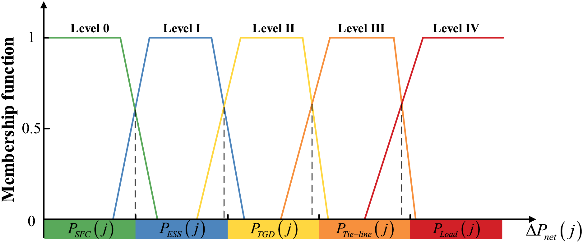
Figure 5: The membership function for early warning

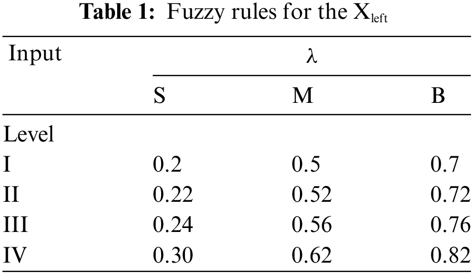
As shown in Fig. 6a, the intersections of the warning membership function with the horizontal axis are referred to as the left intersection and the right intersection, respectively. The two inflection points are referred to as the left inflection point and the right inflection point, respectively. The values of these points are expressed as multiples of the corresponding power intervals. The left and right inflection points are fixed at 0.15 times the power intervals, while the values of the Xleft and Xright are determined by fuzzy rules. Fig. 6b illustrates the membership function curve for the ratio λ of adjacent power intervals, where λ can be expressed as:

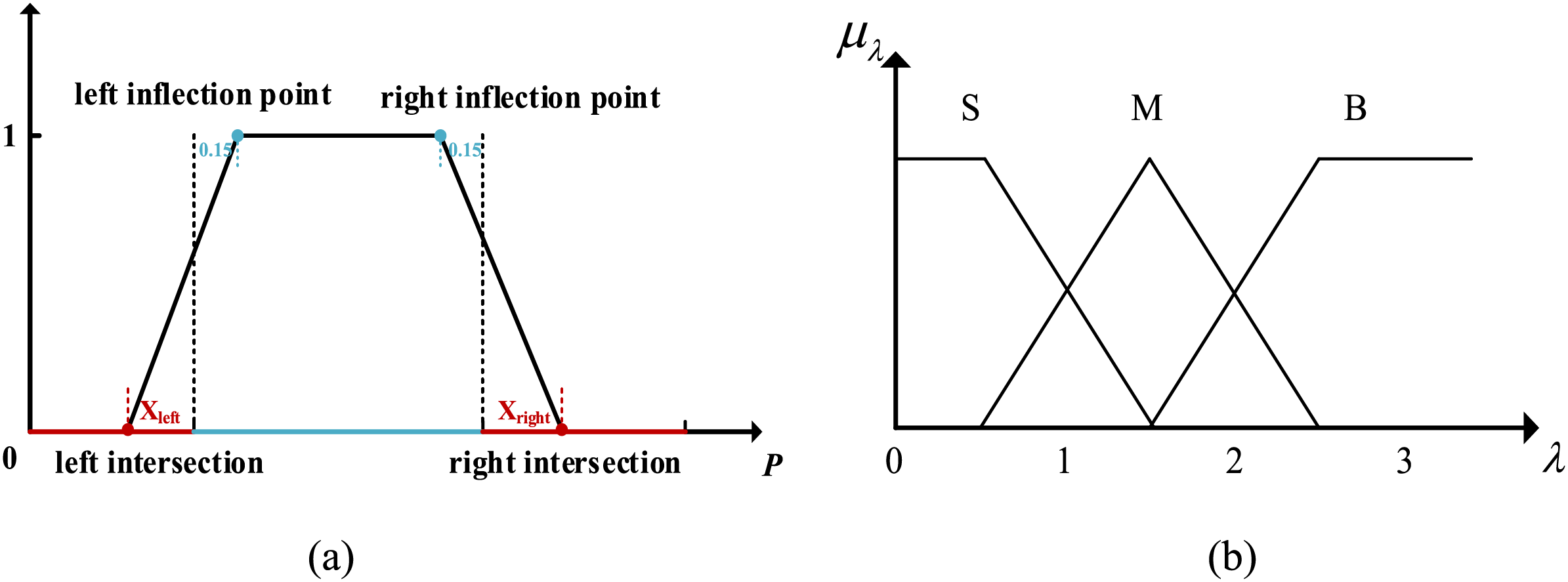
Figure 6: The key information of the membership function. (a) The early warning membership function. (b) The λ membership function

λ=Pi+1Pi(21)

where Pi is the maximum adjustable power capacity of the i-th power control measure. S (small), M (middle), and B (big) for λ are the linguist variables. Under a conservative attitude, the fuzzy rules that take λ and the early warning level of the interval where the intersection point is located as inputs are shown in Tables 1 and 2. If the risk attitude is aggressive, the fuzzy rules for these two intersections need to be swapped.

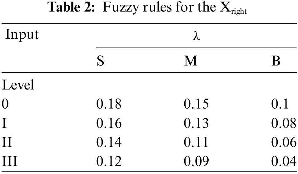
By adjusting the slope of the membership function, the sensitivity to different power intervals is regulated, reflecting the risk attitude of the dispatchers (Fig. 5: The membership function exemplifies a conservative attitude). Finally, the ultimate warning result is derived in accordance with the grading strategy. This method not only captures the risk attitudes of dispatchers but also optimizes the distribution of the adjustable power intervals, thereby reducing the adverse effects of prediction errors.

4.2.3 Warning Level and Corresponding Countermeasure

Based on the fuzzy rules, the power regulation intervals for each power control measure are compared with the grid net load to calculate the warning level of REPREs. The corresponding operating conditions of power system and countermeasures for each warning level are briefly described as follows:

1) Warning Level 0: This indicates that the AGC can achieve the power balance during this period without requiring dispatch control. However, the operation status of AGC units should be monitored to prevent insufficient regulation margin, which may affect power system stability.

2) Warning Level I: This indicates that the dispatchers need to manage the ESS to achieve power balance during this period. Meanwhile, the SOC of the energy storage device should be monitored. If the SOC falls below the lower limit, power output should usually be stopped to extend the lifespan of energy storage device.

3) Warning Level II: This indicates that the dispatchers need to manage the spinning reserve units or start non-spinning units urgently to achieve power balance during this period. The spinning reserve capacity should be monitored, and if it is insufficient or emergency dispatch is required, non-spinning units should be started based on their startup speed and capacity to maintain power system reserve capacity within a safe range.

4) Warning Level III: This indicates that the dispatchers need to carry out inter-area power dispatch to achieve power balance during this period. At this time, the transmission power of tie lines should be monitored to ensure it does not exceed the maximum transmission capacity, ensuring the safety of power transmission.

5) Warning Level IV: This indicates that the existing preventive control measures cannot achieve power balance, and emergency control measures, such as load shedding, need to be implemented to forcibly achieve power balance. During this period, dispatchers should continue implementing preventive control measures to reduce power deficit. Load shedding should prioritize flexible loads to ensure the normal power supply to critical loads as much as possible, minimizing economic losses.

4.3 Solution Procedure of REPRE Early Warning

Early warning results include the risk levels and the adjustable power of each control measure. The solution procedure of REPRE early warning is shown in Fig. 7, including two core parts:

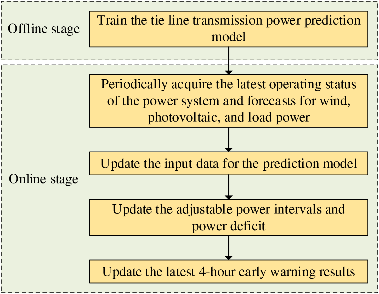
Figure 7: Solution procedure of REPRE early warning

1) Tie line power prediction model training: Based on the historical data of load power, PV power, wind power, and tie line power in the regional grid, the training sample set are generated for the LSTM prediction model, which is trained offline.

2) Periodic update of early warning results: When the operating state of various power control measures or the forecast data of renewable energy and load power is updated, the 4-h warning results, power deficit of power grid, and adjustable power of each measure are updated based on the latest data.

5  Case Studies

In this paper, the regional power grid of a wind-solar-storage base in China is employed to validate the effectiveness of the REPRE early warning method. The grid has an installed PV generating capacity of 10,580 MW, an installed wind generating capacity of 2450 MW, and an installed thermal generating capacity of 7510 MW. The load power ranges between 82 and 128 MW. The installed capacity of energy storage devices is 20% of the rated capacity of renewable energy, capable of providing continuous power supply for 2 h. And there are 22 tie lines with a voltage level of 500 kV and above.

All tests are carried out on a desktop computer with Intel 3.20 GHz Central Processing Unit (CPU) and 16 GB Random Access Memory (RAM).

5.1 Results of Tie Line Selection

The sensitivity of each tie line (parallel lines are merged into a single representation) is calculated by changing the output power of renewable generation in the grid through power flow calculations. With the sensitivity threshold βε = 10%, the selection results are shown in Table 3. Four major tie lines have been identified: Lines 4, 6, 7, and 10. Among them, Lines 6 and 10 represent equivalent lines after consolidation, which show significant changes in transmission power.

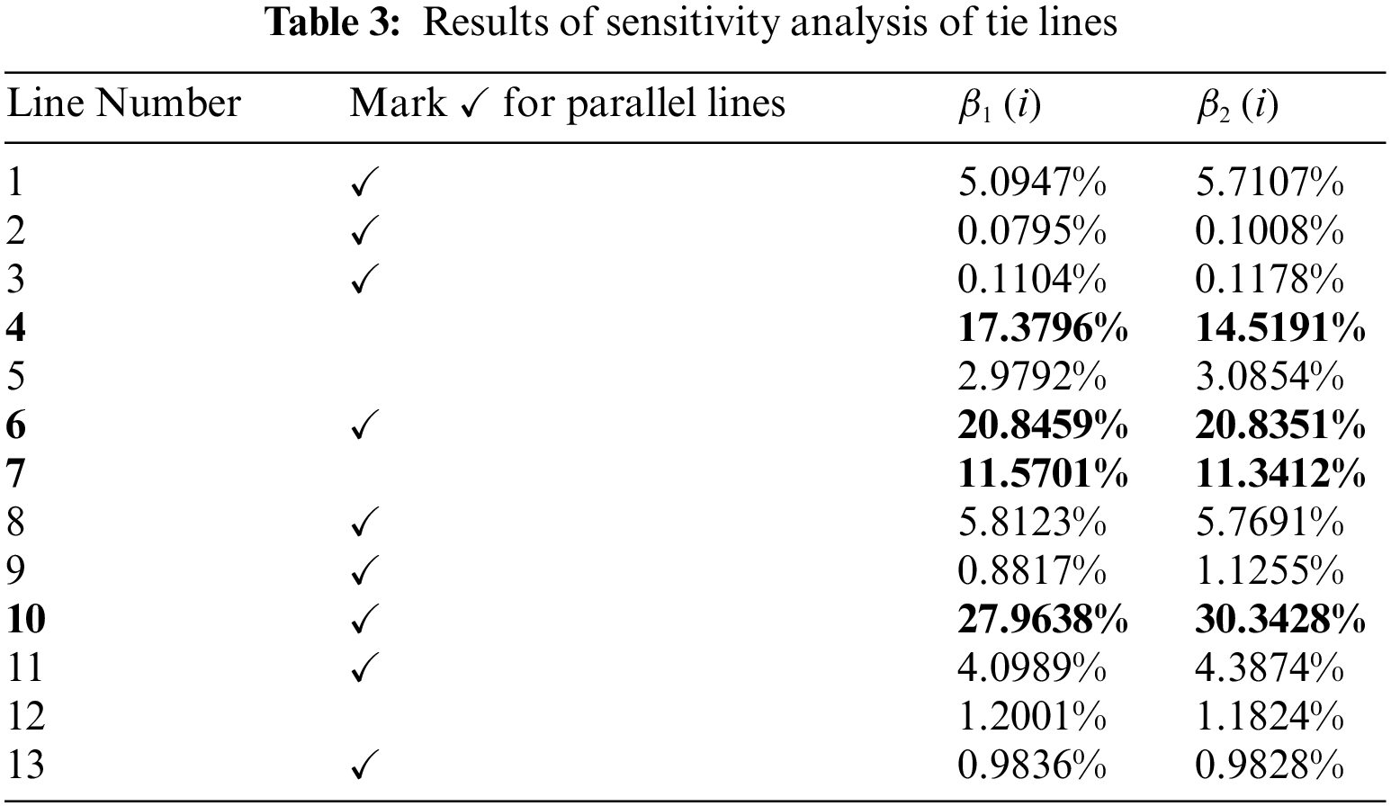
Based on the actual structure of the regional power grid, the selected tie lines are all located in areas with concentrated distribution of renewable energy farms. These tie lines serve as the primary routes for power transmission between the wind-solar-storage base and the external power grids.

5.2 Accuracy Analysis of Prediction Model

In this paper, the PyTorch model library is used to construct prediction models with a prediction time scale of 15 min, 1, 2, and 4 h, using 15-min intervals for the data. The setting of hyperparameters has an essential impact on the convergence speed and prediction accuracy of the LSTM network. The final hyperparameter settings of the prediction model, after continuous optimization, are as follows: the LSTM network consists of two layers with neuron numbers of 20, 20, 25, and 20, respectively; the batch size is 256; the initial learning rate is 0.001; the number of iterations is 400; and the optimization algorithm is Adam’s algorithm. ER2 (Coefficient of Determination), ERMSE (root mean square error, RMSE), and EMAE (mean absolute error, MAE) are selected as the performance evaluation index [40], and the calculation formulas are as follows:

ER2=1−∑i=1N(yi−y⌢i)2∑i=1N(y⌢i−y¯i)2(22)

ERMSE=1N∑i=1N(y⌢i−yi)2(23)

EMAE=1N∑i=1N|y⌢i−yi|(24)

From the above equations, yi, y¯i, and y⌢i denote the samples’ true, average and predicted values, respectively; and N is the number of samples.

The renewable energy, load, and tie line power data of the regional power grid over a year are selected and divided into a training set and a test set with a ratio of 6:4. For each prediction model, the corresponding training subsets and test subsets are generated based on the prediction time scale, and then the hyperparameters are set and the model training is completed. The evaluation indices of each prediction model are shown in Table 4.

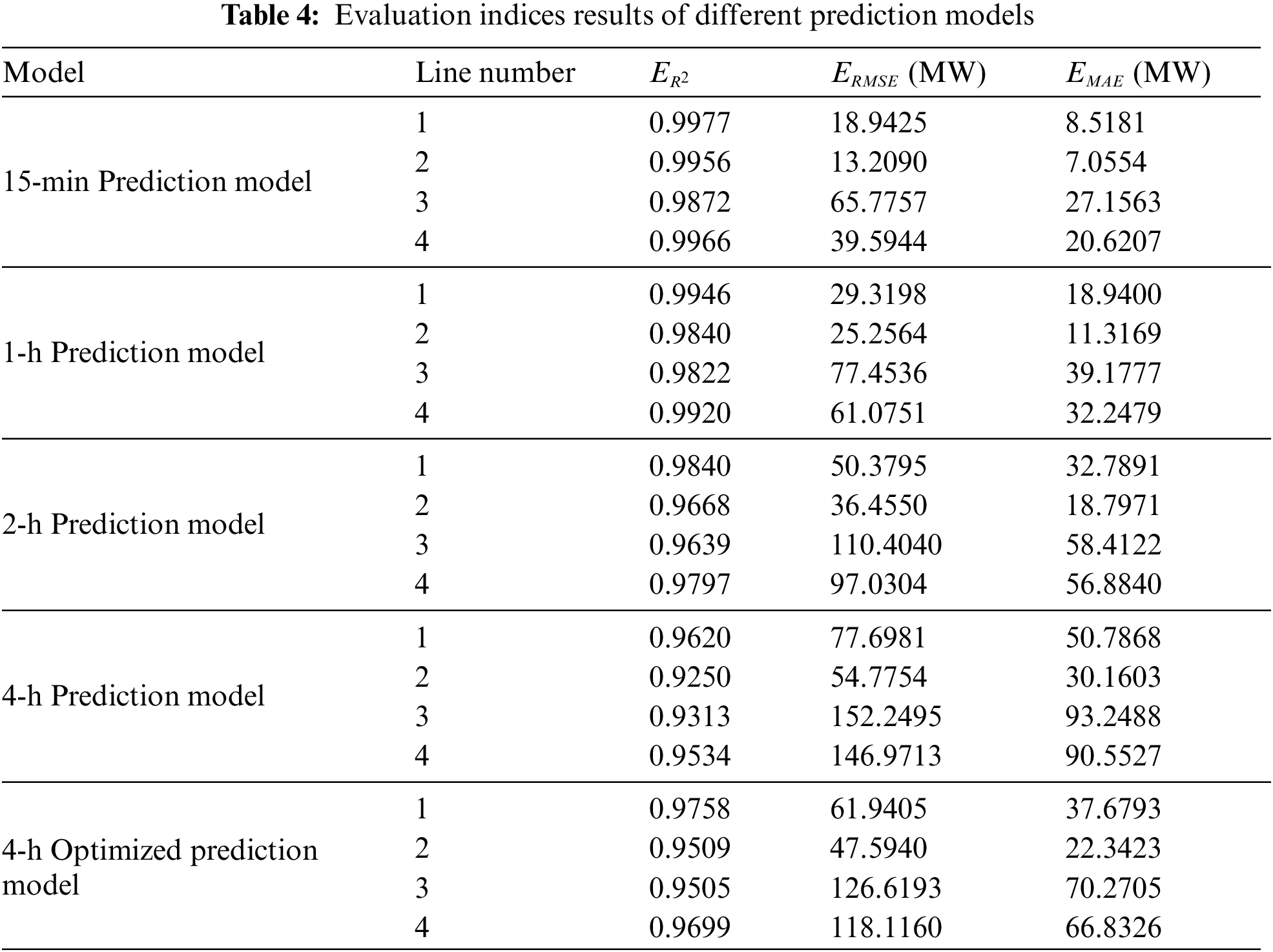
As the prediction time scale increases, the evaluation index ER2 for the power prediction results of the four tie lines gradually decreases, while the indexes ERMSE and EMAE gradually increase, with more pronounced changes. This indicates that the accuracy of the prediction model decreases as the prediction time scale increases. To improve the prediction accuracy of the 4-h tie line power, an optimization method of individual prediction models is implemented. It can be seen that the optimized combination results in index ER2 being closer to 1 and indexes ERMSE and EMAE decreasing significantly compared to the single 4-h prediction time scale model. Thus, the 4-h prediction accuracy of the prediction model is comprehensively improved.

5.3 Effectiveness of Early Warning Method

A typical day is selected as the power ramp event warning calculation object in this section. To simulate power ramp scenarios more realistically, 13:00 is chosen as the start time for the warning calculation. The 24-h historical load power and renewable energy power curves, with a 15-min interval, are shown in Fig. 8. It can be observed that the renewable power at 13:00 is relatively high, making the power system susceptible to severe power ramp events during extreme weather conditions. The 24-h historical power data at the start time of the calculation is used as input data for the prediction model to forecast the tie line power for the next 4 h.

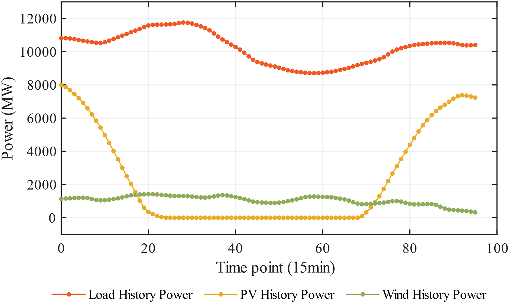
Figure 8: The 24-h history power curves for renewable energy and load power

The historical and predicted power curves for the four tie lines are shown in Fig. 9. In this figure, the interval [−95, 0] represents historical power, while the interval [1,16] represents predicted power data. The positive and negative values of the power depend on whether the power input substation is inside or outside the regional grid. Historical data shows a close correlation between tie line transmission power and renewable energy output power. Therefore, the power dispatch of the tie line is an important means to maintain the power balance of the regional grid where the wind-solar-storage base resides.

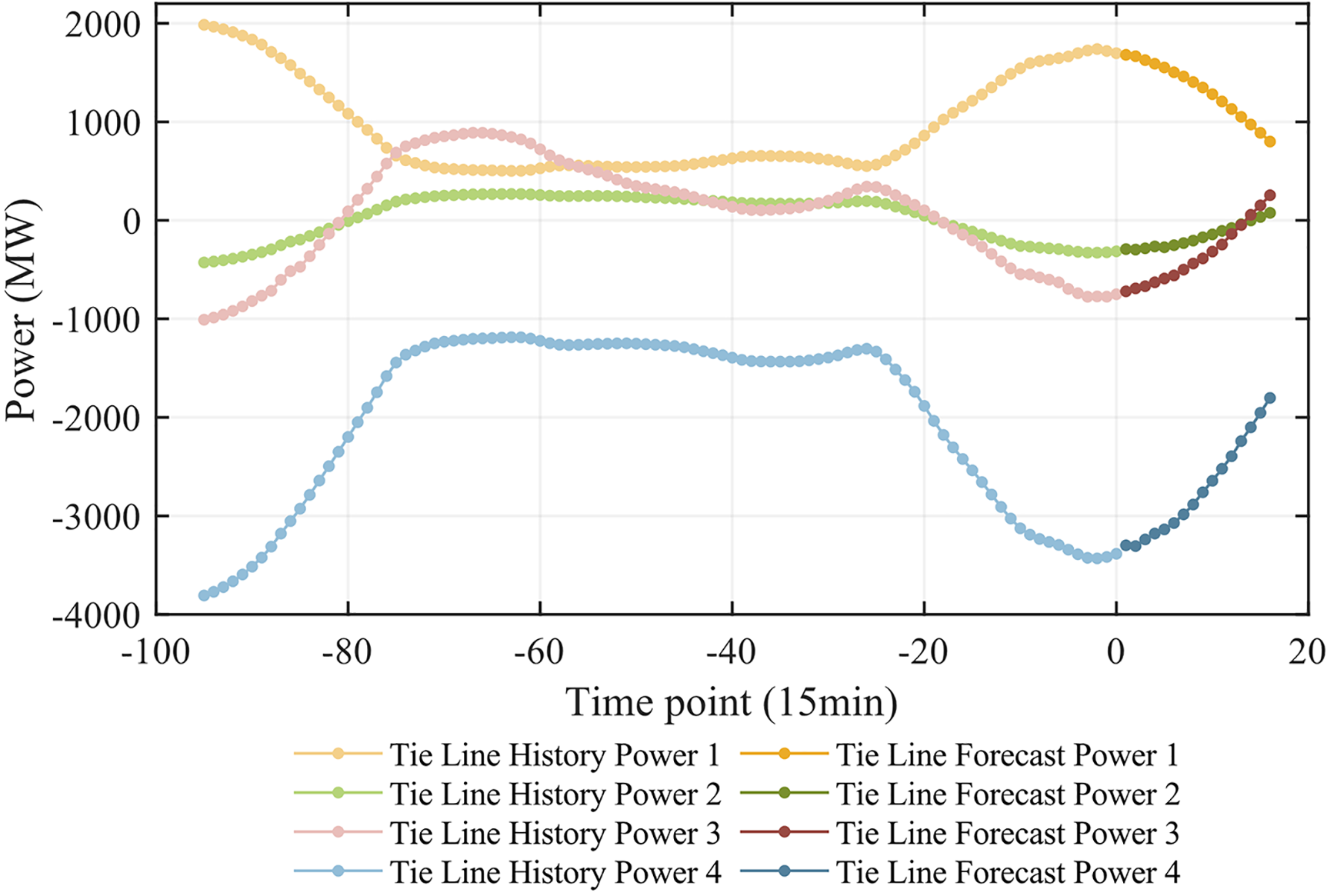
Figure 9: The 24-h history and 4-h forecast power curves for tie lines

5.3.1 Ramping Scenario Construction

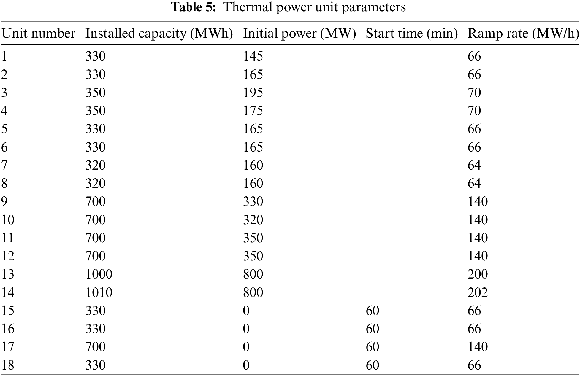
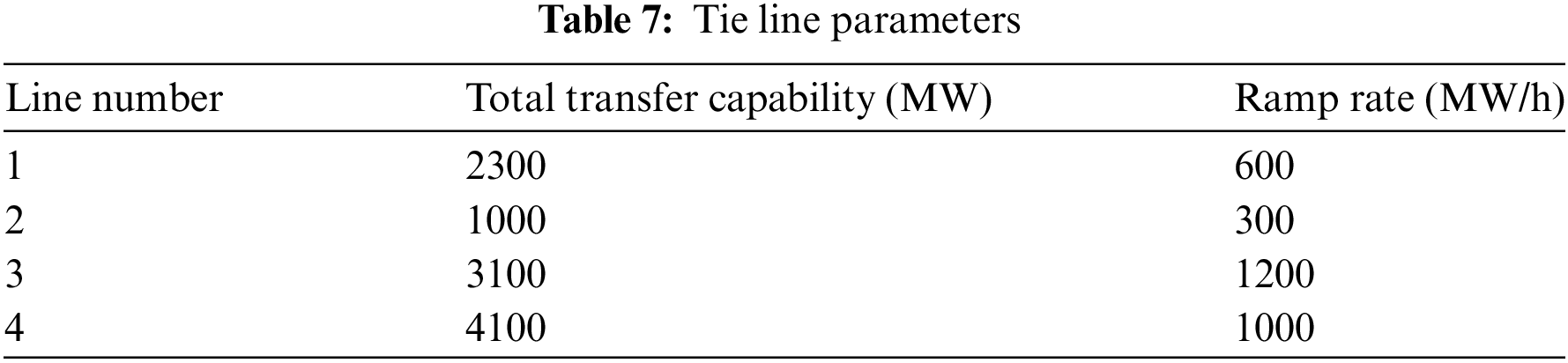
In this section, various power ramp event scenarios are constructed by adjusting the initial operation parameters of each power control measure and using different prediction results of the renewable energy output and load power to verify the effectiveness of the warning method proposed in this paper. The basic operating conditions of the power control measures in the power system are as follows: all the thermal power units in the power system participate in the primary frequency control, while all units except the AGC units participate in the dispatch control; the droop rate for each unit is set at 5%, the load damping coefficient is fixed at 1%, and the allowable frequency deviation range is ±0.1 Hz; the ESS is configured according to the 20% and 2-h standards. Detailed parameter information for the thermal power units, ESS, and tie lines is shown in Tables 5–7, respectively.

Three renewable energy power ramp event scenarios are constructed based on the basic operating scenario of power system.

Case 1: Refer to Fig. 10, we assume that the load forecast increases by 3% in the next hour, by 10% from 1 to 2 h, and by 7% from 2 to 4 h. The PV power forecast decreases by 10% in the next hour, 75% from 1 to 2 h, and 15% from 2 to 4 h. The wind power forecast increases by 15% in the next hour, decreases by 80% from 1 to 2 h, and increases by 70% from 2 to 4 h. Units 1 to 7 are AGC units, units 8 to 14 are spinning reserve units, and the remaining units are non-spinning reserve units. The operating parameters of each power control measure are consistent with those in Tables 5–7.

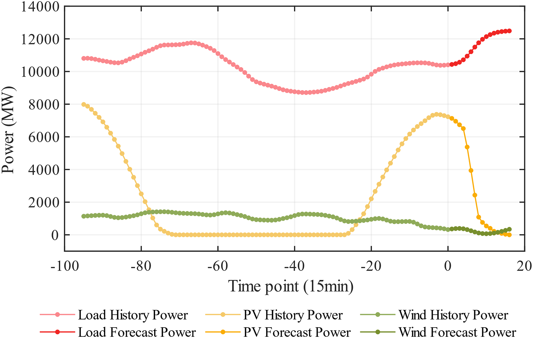
Figure 10: The load and renewable energy power curves for Case 1

Case 2: Based on Case 1, only the initial parameters of the power control measures in the power system are changed without altering load power and renewable energy power. The specific adjustments include the following: Units 8 and 9 are changed to AGC units; the startup times of the non-spinning reserve units are changed to 30, 30, 45, and 45 min, respectively; the initial state of charge of the ESS is set to 0.9. This operating scenario is called Case 2.

Case 3: Based on Case 1, only the load power and the renewable energy power are changed without altering the initial parameters of the power control measures in the power system. The specific adjustments are as follows: The load power is assumed to increase by 3% within the next hour, decrease by 10% from the 1st to the 2nd h, and increase by 10% from the 2nd to the 4th h; no adjustments are made to the renewable energy power, and other parameters remain the same as in Case 1. This operating scenario is called Case 3.

5.3.2 Results of Adjustable Power for Different Operating States

For the three renewable energy power ramp scenarios constructed in Section 5.3.1, the power deficit of the grid and the adjustable power capacity of power control measures are calculated separately. The calculation results are then analyzed in conjunction with the corresponding operational scenarios.

The calculation results of Case 1 are shown in Fig. 11. The first set of bars represents the active power deficit of power grid for each period. In Periods 5 to 8, the power ramp process of the renewable energy power is relatively intense, and the change direction of the load power is opposite to the ramp direction of the renewable energy power, resulting in a significant power deficit of the power grid, which exceeds 6500 MW. The following four sets of bar graphs sequentially represent the adjustable power capacity of AGC, ESS, thermal generation dispatch, and tie line power dispatch for each period. Due to the limited reserve capacity of the AGC units, AGC loses its regulation capability after the 12th period. Similarly, due to the SOC limitations, the ESS loses its regulation capability after the 9th period. In contrast, the thermal power reserve units and tie lines always maintain a certain power regulation capability. The dispatch control of thermal power units reaches its maximum regulation capability in the 5th period and gradually decreases thereafter, while the tie lines always have sufficient power regulation capability.

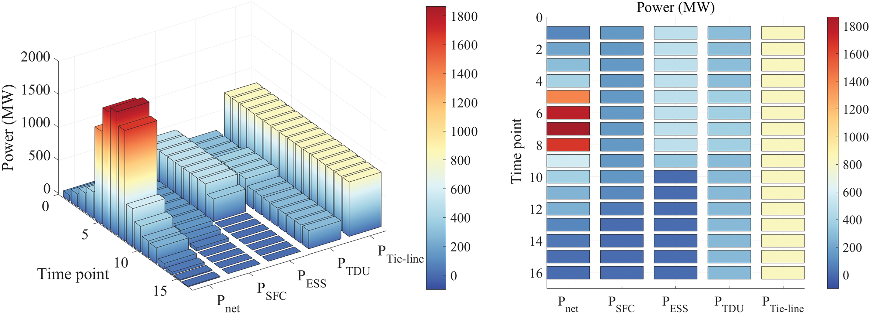
Figure 11: The calculation results of power deficit and adjustable power capacity in Case 1

The calculation results of Case 2 are shown in Fig. 12. The active power deficit of the power grid in each period is the same as that in Case 1, and only the control capability of the power control measures is different. First, the number of AGC units has increased, which improves the regulation capability of AGC. Second, the initial state of charge of ESS has increased, which allows it to maintain regulation capability for 4 h. Finally, the start-up time of the non-spinning reserves has been reduced, which improves the response speed of the non-spinning reserves, and the dispatch control of the thermal power units reaches its maximum control capability in the 4th period.

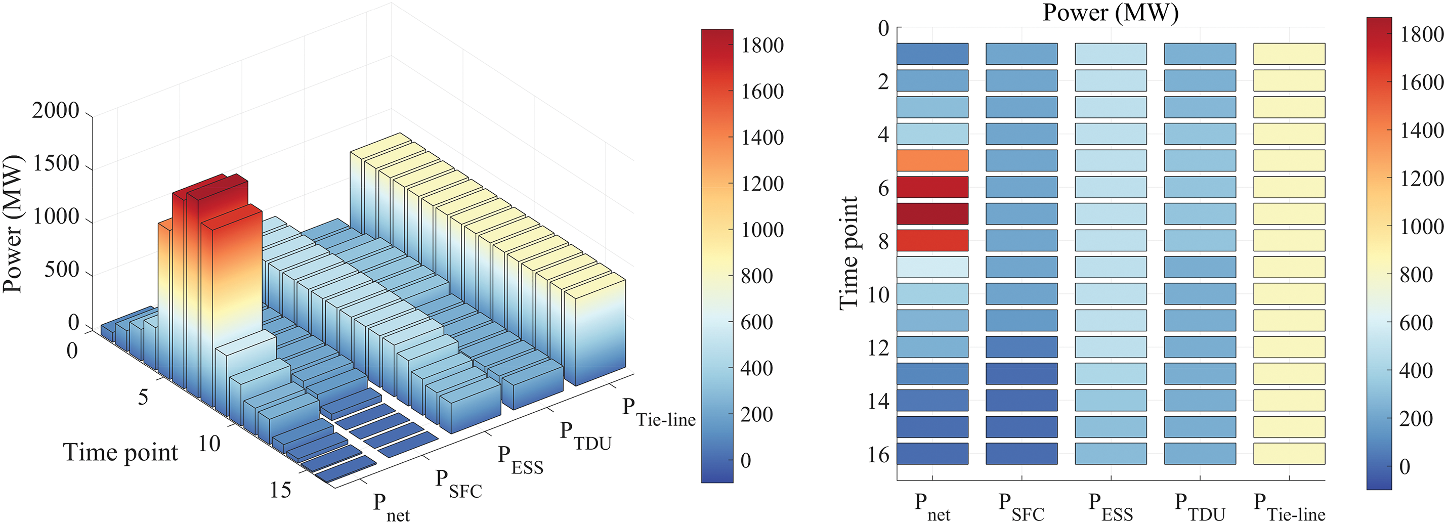
Figure 12: The calculation results of power deficit and adjustable power capacity in Case 2

The calculation results of Case 3 are shown in Fig. 13. Compared with Case 1, during periods 5 to 8, when the power ramping process of renewable energy is most severe, the change direction of load power is the same as the ramping direction of renewable energy power, which counteracts the effect of each other, resulting in a substantial reduction of the power deficit of the grid, only 4800 MW. However, from the 9th period, the load power of the grid gradually increases, and the magnitude of load change in Case 3 is larger, leading to an increased active power deficit of the grid in subsequent periods.

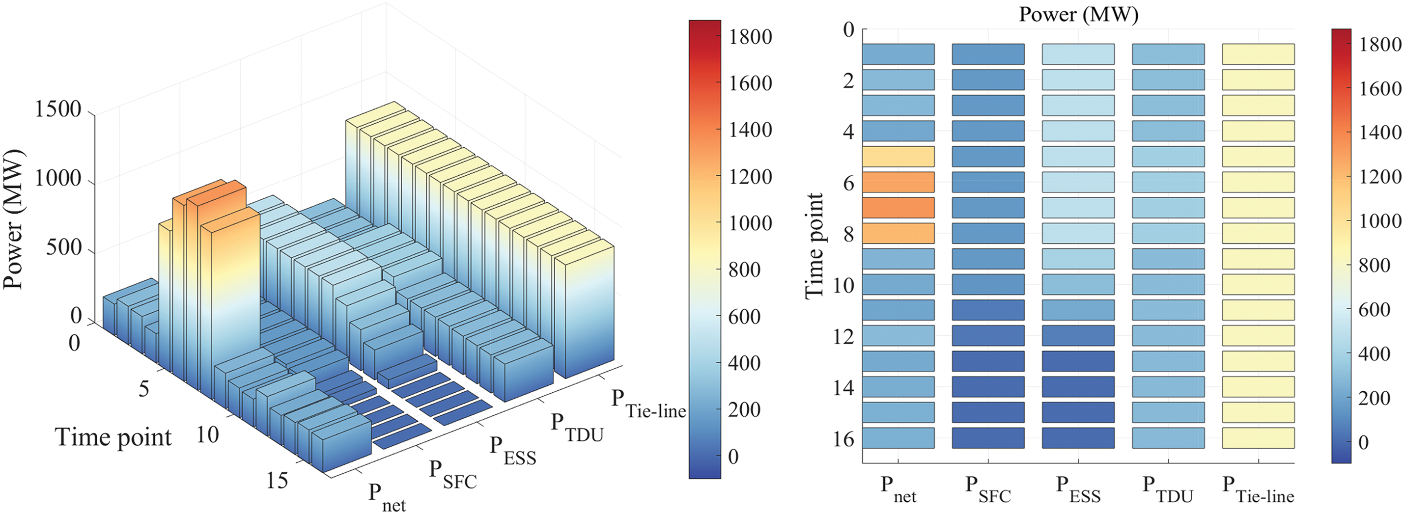
Figure 13: The calculation results of power deficit and adjustable power capacity in Case 3

5.3.3 Analysis of Early Warning Result

Using the conservative warning strategy, the results of the REPREs under three different operating scenarios are shown in Fig. 14. The comparative analysis of the warning results is as follows:

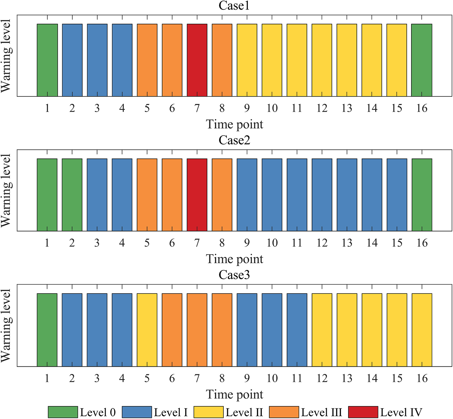
Figure 14: The results of REPRE early warning

1) In Case 2, more AGC units and fast start units are used than in Case 1, and the capacity of the ESS is increased. This increases the tolerance of power system to REPREs and reduces their negative impact. As a result, the overall warning level throughout the event is lower in Case 2 than in Case 1.

In the early stages of the ramp event, Case 2 has more AGC units, ensuring the power balance of the power grid only by the AGC in the first two periods. Notably, from Periods 5 to 8, the warning level remains at Level IV during Period 7. Although the rapid response capability and reserve capacity of the power system are improved in Case 2, there is no improvement in the maximum ramp rate of the control measures. During Period 7, the control capabilities of all power control measures reach their limits, similar to Case 1, resulting in the same warning level. This indicates that the power ramp process during this period is extremely severe, and the preventive control measures alone cannot guarantee the power balance of power grid. Dispatchers must implement emergency control measures or reduce the output of renewable energy in advance to minimize the power deficit during this period. From Periods 9 to 15, the ESS in Case 2 still has sufficient power regulation capability to maintain power balance without the need for reserve units, resulting in one level lower than in Case 1. In Period 16, there is a negative power deficit, so warning level is 0.

2) In Case 1, during Periods 5 to 8, the renewable energy down-ramp process coincides with the load increase phase, exacerbating the effect and significantly increasing the power deficit, ultimately leading to a Level IV warning, which severely impacts the power system. However, in Case 3, during the same periods, the renewable energy down-ramp process coincides with the load decrease phase, offsetting each other and significantly reducing the power deficit, resulting in a lower overall warning level and less damage to the power system.

In Periods 9 to 11, due to the reduced severity of the overall ramp event in the previous periods, the consumption of reserve capacity in the power system decreases. This allows the ESS to maintain sufficient power regulation capability, resulting in a relatively lower warning level. From Periods 12 to 15, the ESS loses its power regulation capability and the thermal power reserve units take control, with a warning level of II. In Period 16, the warning level remains at II due to the significant increase in load and insufficient AGC and ESS reserve capacity.

Therefore, it is necessary to configure and maintain sufficient fast-responding power sources, such as energy storage systems, pumped storage plants, and gas turbine units, for power systems with high penetration of renewable energy. This prevents the adverse effects of REPREs on the power system, thereby increasing system security and stability. Additionally, the impact of the same degree of renewable energy power ramp process on the power system varies significantly under different load changes. In particular, when the two effects overlap each other, it leads to severe power imbalance in the power system. Therefore, merely analyzing the characterization of the renewable energy ramp process (such as ramp amplitude, ramp rate, etc.) and using a fixed threshold to measure the risk of ramp events without considering load changes fails to accurately reflect the risk status of the power system.

In summary, the early warning method proposed in this paper can provide early warnings for REPREs under different operating conditions of the control measures and load changes. Dispatchers can adjust the membership function according to their own risk attitude to obtain corresponding levels of ramp event warnings. Furthermore, the method provides the maximum adjustable power capacity for different power control measures in different periods, enabling dispatchers to comprehensively grasp the operating status and risk trends of the power system. This guides them to adopt the correct dispatch strategy to minimize the negative impact of REPREs on the system. The early warning results of different case studies fully demonstrate the effectiveness of the early warning method presented in this paper.

5.4 Comparison with Other Methods

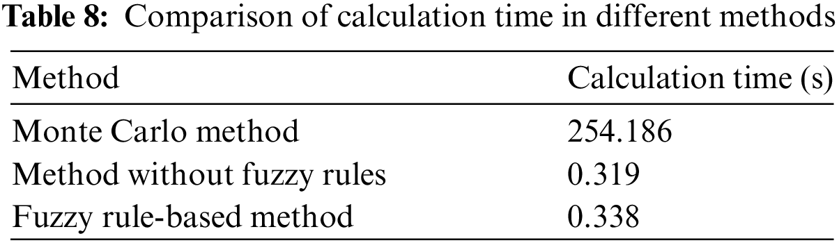
This section presents a comparative analysis of the proposed method, the Monte Carlo method, and the method without fuzzy rules in addressing uncertainty in the warning process. The experiment adopts the parameters of Case 1, assuming a renewable energy power prediction error of 15% and a load prediction error of 5%, both following a normal distribution. The risk aversion rate of the dispatchers is set at 90%, meaning that when the probability of higher warning level exceeds 10%, the result is classified as the higher warning level. The Monte Carlo method uses 5000 samples to calculate the probability of warning results for each period based on frequency. The simulation results are shown in Fig. 15 and Table 8, where each period’s three baseline bars represent the Monte Carlo method, the method without fuzzy rules, and the proposed method. The dashed line indicates the risk aversion rate of the Monte Carlo method.

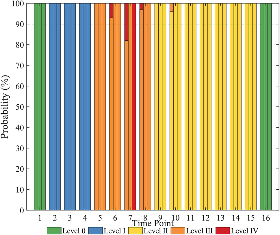
Figure 15: Comparison of warning results in different methods

From Fig. 15, it can be observed that, except for the 7th period, the warning results of the three methods are consistent in other periods. The Monte Carlo method, when the sample size is sufficiently large, can cover almost all power ramp scenarios, resulting in high simulation accuracy. Therefore, the warning results of the Monte Carlo method are considered accurate. According to the probabilities of the Monte Carlo method’s warning results, in the operating scenario of Case 1, the net load ΔPnet during the 6th, 7th, 8th, and 10th periods falls on the boundary of the warning interval. The high warning level probabilities for these periods are 7%, 18%, 3%, and 4%, respectively. Under the constraint of a 90% risk aversion rate, the final warning levels are III, IV, III, and II, respectively, which are consistent with the results of the proposed method. However, the method without fuzzy rules assigns a warning level of III for the 7th period, indicating its inability to accurately handle boundary values of the warning interval and provide effective warning results consistent with the dispatcher’s risk attitude.

As shown in Table 8, the Monte Carlo method demands a substantial number of samples, leading to extended computation times. In contrast, the proposed method, which uses fuzzy rules to address uncertainty, requires only one calculation, significantly reducing the computation time. Therefore, the fuzzy rule-based warning system not only effectively warn of REPREs and provide warning results consistent with the risk attitude of dispatchers but also ensures rapid computation, meeting the needs of online operation.

5.5 Practical Application of REPRE Early Warning System

To implement the proposed REPRE early warning system in an actual power grid, two primary challenges must be addressed: (1) acquisition of power data and operational status information from the power grid; (2) adaptability of the tie line power prediction model.

To address these challenges, the application schematic of the REPRE early warning system is illustrated in Fig. 16. Firstly, the energy management system conducts real-time monitoring of power grid data and operational information, packaging and transmitting this data to both the historical database and the warning system. Subsequently, the database categorizes the received data, selecting time series data for renewable energy generation, load, and tie line power. Dispatchers obtain power data from the database to form training set samples for offline training of the tie line power prediction model, ensuring the prediction model matches the target power grid. Finally, based on their risk attitude towards REPREs, dispatchers choose the fuzzy rule parameters of the REPRE early warning system, completing the initialization and tuning of the warning system.

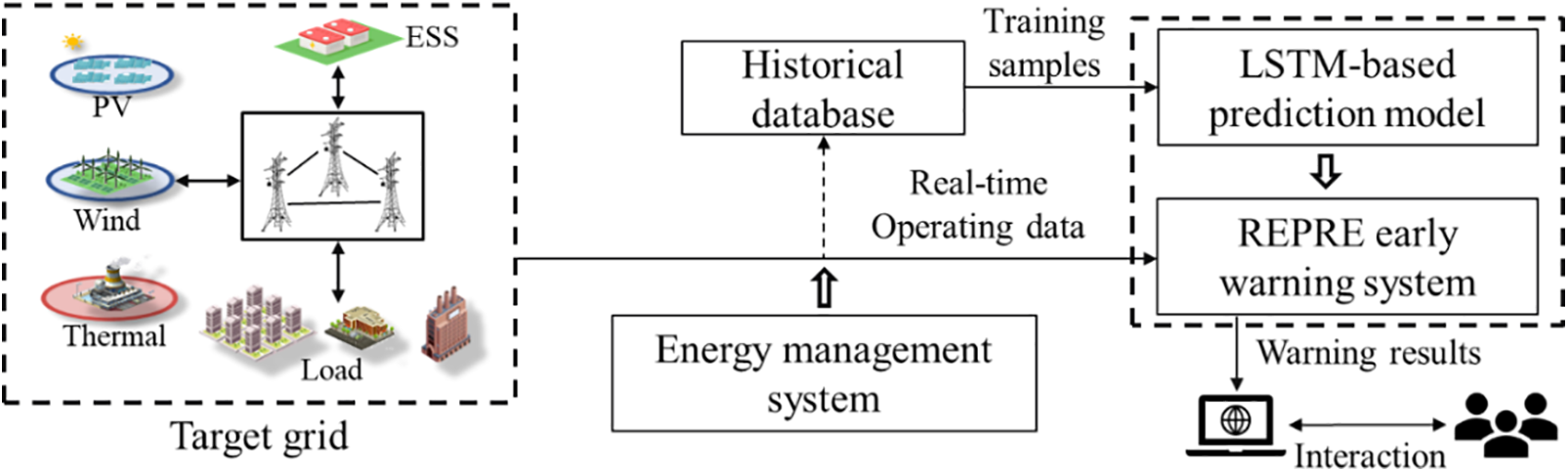
Figure 16: The application schematic of the REPRE early warning system

During system operation, whenever the energy management system updates the power and operational data of power grid, the warning system updates the warning results for the upcoming 4-h power ramp events and the power adjustment capabilities of various power control measures based on the latest data. Through the initialization and tuning of the warning system, dispatchers can obtain warning results aligned with their own judgments without considering risk level probabilities. This enables faster formulation of appropriate preventive control strategies and reduces the adverse impacts of REPREs.

6  Conclusion

This paper proposes an early warning method for wind and photovoltaic power ramp events based on the LSTM network and fuzzy rule. The following conclusions are drawn from both theoretical analysis and numerical studies.

1) Based on the control costs of various power control measures in the grid, a ranking strategy for the severity of REPREs is proposed, facilitating a robust decision-making framework for subsequent prevention and control decisions.

2) The prediction model for tie line power is established based on LSTM network, determining the power support capacity of the external grid and improving the accuracy of 4-h forecast results.

3) The early warning method based on fuzzy rules is applicable to different operating scenarios. The warning results match the risk attitudes of dispatchers to the REPREs, effectively guiding preventive control decisions.

The quantitative relationship between preventive control measures and warning risks of REPREs will be focused on in future studies, considering source-network-load-storage coordination. This aims to more accurately and effectively guide decision-making in control strategies.

Acknowledgement: We would like to thank all collaborators who have made outstanding contributions to this article, as well as the support of the relevant staff of the Energy Engineering journal.

Funding Statement: This research was funded by State Grid Shandong Electric Power Company Technology Project (520626220110).

Author Contributions: The authors confirm contribution to the paper as follows: study conception and design: Huan Ma, Linlin Ma, Zengwei Wang, Yutian Liu; data collection: Zhendong Li, Yuanzhen Zhu; analysis and interpretation of results: Huan Ma, Zengwei Wang, Yutian Liu; draft manuscript preparation: Huan Ma, Linlin Ma, Zengwei Wang, Zhendong Li, Yuanzhen Zhu. All authors reviewed the results and approved the final version of the manuscript.

Availability of Data and Materials: We hereby declare that the data used in the article comes from the State Grid Shandong Electric Power Research Institute and is accompanied by a confidentiality. We cannot directly provide the dataset.

Ethics Approval: This study did not involve human or animal subjects, and therefore, does not require ethical approval.

Conflicts of Interest: The authors declare that they have no conflicts of interest to report regarding the present study.

References

1. J. Kabouris and F. D. Kanellos, “Impacts of large-scale wind penetration on designing and operation of electric power systems,” IEEE Trans. Sustain. Energy, vol. 1, no. 2, pp. 107–114, Jul. 2010. doi: 10.1109/TSTE.2010.2050348. [Google Scholar] [CrossRef]

2. M. Karimi, H. Mokhlis, K. Naidu, S. Uddin, and A. H. A. Bakar, “Photovoltaic penetration issues and impacts in distribution network–A review,” Renew. Sustain. Energy Rev., vol. 53, pp. 594–605, Jan. 2016. doi: 10.1016/j.rser.2015.08.042. [Google Scholar] [CrossRef]

3. T. Ouyang, X. Zha, L. Qin, Y. He, and Z. Tang, “Prediction of wind power ramp events based on residual correction,” Renew. Energy, vol. 136, pp. 781–792, Jun. 2019. doi: 10.1016/j.renene.2019.01.049. [Google Scholar] [CrossRef]

4. Y. Liu, R. Fan, and V. Terzija, “Power system restoration: A literature review from 2006 to 2016,” J. Mod. Power Syst. Clean Energy, vol. 4, no. 3, pp. 332–341, Jul. 2016. doi: 10.1007/s40565-016-0219-2. [Google Scholar] [CrossRef]

5. M. Ni, J. D. McCalley, V. Vittal, and T. Tayyib, “Online risk-based security assessment,” IEEE Trans. Power Syst., vol. 18, no. 1, pp. 258–265, Feb. 2003. doi: 10.1109/TPWRS.2002.807091. [Google Scholar] [CrossRef]

6. Y. Fujimoto, Y. Takahashi, and Y. Hayashi, “Alerting to rare large-scale ramp events in wind power generation,” IEEE Trans. Sustain. Energy., vol. 10, no. 1, pp. 55–65, Jan. 2019. doi: 10.1109/TSTE.2018.2822807. [Google Scholar] [CrossRef]

7. F. Sanchez-Sutil, A. Cano-Ortega, J. C. Hernandez, and C. Rus-Casas, “Development and calibration of an open source, low-cost power smart meter prototype for PV household-prosumers,” Electronics, vol. 8, no. 8, Aug. 2019, Art. no. 878. doi: 10.3390/electronics8080878. [Google Scholar] [CrossRef]

8. A. Couto, P. Costa, L. Rodrigues, V. V. Lopes, and A. Estanqueiro, “Impact of weather regimes on the wind power ramp forecast in Portugal,” IEEE Trans. Sustain. Energy., vol. 6, no. 3, pp. 934–942, Jul. 2015. doi: 10.1109/TSTE.2014.2334062. [Google Scholar] [CrossRef]

9. L. Cheng, H. Zang, A. Trivedi, D. Srinivasan, Z. Wei and G. Sun, “Mitigating the impact of photovoltaic power ramps on intraday economic dispatch using reinforcement forecasting,” IEEE Trans. Sustain. Energy., vol. 15, no. 1, pp. 3–12, Jan. 2024. doi: 10.1109/TSTE.2023.3261444. [Google Scholar] [CrossRef]

10. H. Ma, C. Li, and Y. Liu, “Multi-level early warning method for wind power ramp events,” Autom. Electr. Power Syst., vol. 41, no. 11, pp. 39–47, Jun. 2017. doi: 10.7500/AEPS20161021008. [Google Scholar] [CrossRef]

11. Y. Qi and Y. Liu, “Wind power ramping control using competitive game,” IEEE Trans. Sustain. Energy., vol. 7, no. 4, pp. 1516–1524, Oct. 2016. doi: 10.1109/TSTE.2016.2558584. [Google Scholar] [CrossRef]

12. Y. Qi, Y. Liu, and Q. Wu, “Non-cooperative regulation coordination based on game theory for wind farm clusters during ramping events,” Energy, vol. 132, pp. 136–146, Aug. 2017. doi: 10.1016/j.energy.2017.05.060. [Google Scholar] [CrossRef]

13. Z. Wang, Z. Li, Y. Liu, and H. Ma, “Wind and PV power ramp events prediction based on long short-term memory network,” presented at the 2023 IEEE Sustain. Power Energy Conf., Chongqing, China, Nov. 28–30, 2023, pp. 989–993. [Google Scholar]

14. Z. Liang et al., “Assessment of wind power ramp events based on stacked denoising autoencoder,” presented at the 2019 8th IEEE Int. Conf. Adv. Power Syst. Autom. Prot., Xi’an, China, Oct. 21–24, 2019, pp. 1031–1035. [Google Scholar]

15. R. Diao, V. Vittal, and N. Logic, “Design of a real-time security assessment tool for situational awareness enhancement in modern power systems,” IEEE Trans. Power Syst., vol. 25, no. 2, pp. 957–965, May 2010. doi: 10.1109/TPWRS.2009.2035507. [Google Scholar] [CrossRef]

16. S. Datta and V. Vittal, “Operational risk metric for dynamic security assessment of renewable generation,” IEEE Trans. Power Syst., vol. 32, no. 2, pp. 1389–1399, Mar. 2017. doi: 10.1109/TPWRS.2016.2577500. [Google Scholar] [CrossRef]

17. M. T. Lawder et al., “Battery ESS (BESS) and battery management system (BMS) for grid-scale applications,” Proc. IEEE, vol. 102, no. 6, pp. 1014–1030, Jun. 2014. doi: 10.1109/JPROC.2014.2317451. [Google Scholar] [CrossRef]

18. N. M. Kumar, A. Ghosh, and S. S. Chopra, “Power resilience enhancement of a residential electricity user using photovoltaics and a battery energy storage system under uncertainty conditions,” Energies, vol. 13, no. 16, Aug. 2020, Art. no. 4193. doi: 10.3390/en13164193. [Google Scholar] [CrossRef]

19. Y. Gong, Q. Jiang, and R. Baldick, “Ramp event forecast based wind power ramp control with ESS,” IEEE Trans. Power Syst., vol. 31, no. 3, pp. 1831–1844, May 2016. doi: 10.1109/TPWRS.2015.2445382. [Google Scholar] [CrossRef]

20. L. S. Vargas, G. Bustos-Turu, and F. Larraín, “Wind power curtailment and energy storage in transmission congestion management considering power plants ramp rates,” IEEE Trans. Power Syst., vol. 30, no. 5, pp. 2498–2506, Sep. 2015. doi: 10.1109/TPWRS.2014.2362922. [Google Scholar] [CrossRef]

21. X. Zheng et al., “Loss-minimizing generation unit and tie-line scheduling for asynchronous interconnection,” IEEE J. Emerg. Sel. Topics Power Electron., vol. 6, no. 3, pp. 1095–1103, Sep. 2018. doi: 10.1109/JESTPE.2017.2783930. [Google Scholar] [CrossRef]

22. A. Alassi, S. Bañales, O. Ellabban, G. Adam, and C. MacIver, “HVDC transmission: Technology review, market trends and future outlook,” Renew. Sustain. Energy Rev., vol. 112, pp. 530–554, Sep. 2019. doi: 10.1016/j.rser.2019.04.062. [Google Scholar] [CrossRef]

23. Y. Huang, Y. Wang, and N. Liu, “A two-stage energy management for heat-electricity integrated energy system considering dynamic pricing of Stackelberg game and operation strategy optimization,” Energy, vol. 244, Apr. 2022, Art. no. 122576. doi: 10.1016/j.energy.2021.122576. [Google Scholar] [CrossRef]

24. P. Lara-Benítez, M. Carranza-García, and J. C. Riquelme, “An experimental review on deep learning architectures for time series forecasting,” Int. J. Neural Syst., vol. 31, no. 3, Mar. 2021, Art. no. 2130001. doi: 10.1142/S0129065721300011. [Google Scholar] [PubMed] [CrossRef]

25. Y. Cui, Z. Chen, Y. He, X. Xiong, and F. Li, “An algorithm for forecasting day-ahead wind power via novel long short-term memory and wind power ramp events,” Energy, vol. 263, Jan. 2023, Art. no. 125888. doi: 10.1016/j.energy.2022.125888. [Google Scholar] [CrossRef]

26. F. Wang, Z. Xuan, Z. Zhen, K. Li, T. Wang and M. Shi, “A day-ahead PV power forecasting method based on LSTM-RNN model and time correlation modification under partial daily pattern prediction framework,” Energy Convers. Manag., vol. 212, May. 2020, Art. no. 112766. doi: 10.1016/j.enconman.2020.112766. [Google Scholar] [CrossRef]

27. Y. Liu, P. Zhang, and X. Qiu, “Optimal volt/var control in distribution systems,” Int. J. Electr. Power Energy Syst., vol. 24, no. 4, pp. 271–276, May 2002. doi: 10.1016/S0142-0615(01)00032-1. [Google Scholar] [CrossRef]

28. X. -C. Shangguan, Y. He, C. -K. Zhang, L. Jiang, and M. Wu, “Adjustable event-triggered load frequency control of power systems using control-performance-standard-based fuzzy logic,” IEEE Trans. Fuzzy Syst., vol. 30, no. 8, pp. 3297–3311, Aug. 2022. doi: 10.1109/TFUZZ.2021.3112232. [Google Scholar] [CrossRef]

29. B. Mohandes, M. S. E. Moursi, N. Hatziargyriou, and S. E. Khatib, “A review of power system flexibility with high penetration of renewables,” IEEE Trans. Power Syst., vol. 34, no. 4, pp. 3140–3155, Jul. 2019. doi: 10.1109/TPWRS.2019.2897727. [Google Scholar] [CrossRef]

30. J. Yan, C. Li, and Y. Liu, “Insecurity early warning for large scale hybrid AC/DC grids based on decision tree and semi-supervised deep learning,” IEEE Trans. Power Syst., vol. 36, no. 6, pp. 5020–5031, Nov. 2021. doi: 10.1109/TPWRS.2021.3071918. [Google Scholar] [CrossRef]

31. B. Li, S. Wang, B. Li, H. Li, and J. Wu, “Optimal performance evaluation of thermal AGC units based on multi-dimensional feature analysis,” Appl. Energy., vol. 339, Jun. 2023, Art. no. 120994. doi: 10.1016/j.apenergy.2023.120994. [Google Scholar] [CrossRef]

32. A. Kargarian, G. Hug, and J. Mohammadi, “A multi-time scale co-optimization method for sizing of energy storage and fast-ramping generation,” IEEE Trans. Sustain. Energy., vol. 7, no. 4, pp. 1351–1361, Oct. 2016. doi: 10.1109/TSTE.2016.2541685. [Google Scholar] [CrossRef]

33. L. Wu, “A transformation-based multi-area dynamic economic dispatch approach for preserving information privacy of individual areas,” IEEE Trans. Smart Grid, vol. 10, no. 1, pp. 722–731, Jan. 2019. doi: 10.1109/TSG.2017.2751479. [Google Scholar] [CrossRef]

34. S. S. Reddy, “Multi-objective based congestion management using generation rescheduling and load shedding,” IEEE Trans. Power Syst., vol. 32, no. 2, pp. 852–863, Mar. 2017. doi: 10.1109/TPWRS.2016.2569603. [Google Scholar] [CrossRef]

35. O. E. Moya, “A spinning reserve, load shedding, and economic dispatch solution by bender’s decomposition,” IEEE Trans. Power Syst., vol. 20, no. 1, pp. 384–388, Feb. 2005. doi: 10.1109/TPWRS.2004.831675. [Google Scholar] [CrossRef]

36. B. -W. Yi, J. -H. Xu, and Y. Fan, “Inter-regional power grid planning up to 2030 in China considering renewable energy development and regional pollutant control: A multi-region bottom-up optimization model,” Appl. Energy, vol. 184, pp. 641–658, Dec. 2016. doi: 10.1016/j.apenergy.2016.11.021. [Google Scholar] [CrossRef]

37. X. Chen, Y. Du, H. Wen, L. Jiang, and W. Xiao, “Forecasting-based power ramp-rate control strategies for utility-scale PV systems,” IEEE Trans. Ind. Electron., vol. 66, no. 3, pp. 1862–1871, Mar. 2019. doi: 10.1109/TIE.2018.2840490. [Google Scholar] [CrossRef]

38. J. Zhang, C. Lu, J. Song, and J. Zhang, “Real-time AGC dispatch units considering wind power and ramping capacity of thermal units,” J. Mod. Power Syst. Clean Energy, vol. 3, no. 3, pp. 353–360, Sep. 2015. doi: 10.1007/s40565-015-0141-z. [Google Scholar] [CrossRef]

39. W. Zhang and Y. Liu, “Multi-objective reactive power and voltage control based on fuzzy optimization strategy and fuzzy adaptive particle swarm,” Int. J. Electr. Power Energy Syst., vol. 30, no. 9, pp. 525–532, Nov. 2008. doi: 10.1016/j.ijepes.2008.04.005. [Google Scholar] [CrossRef]

40. J. Zhang, M. Cui, B. -M. Hodge, A. Florita, and J. Freedman, “Ramp forecasting performance from improved short-term wind power forecasting over multiple spatial and temporal scales,” Energy, vol. 122, pp. 528–541, Mar. 2017. doi: 10.1016/j.energy.2017.01.104. [Google Scholar] [CrossRef]