Probabilistic Calculation of Tidal Currents for Wind Powered Systems Using PSO Improved LHS

1  Introduction

With the significant promotion of wind power generation in China, wind turbines in grid-connected operations have introduced challenges such as voltage fluctuations and substantial harmonic pollution [1], which adversely impact the stability of grid operations. The reliable operation of power systems is susceptible to several uncertainties, which can complicate both the planning and operational phases. To assess these impacts comprehensively, Borkows introduced the concept of Probabilistic Load Flow (PLF) in 1974 [2].

In the four decades following the introduction of PLF, both domestic and international scholars have proposed various calculation methods. Currently, there are three primary categories of methods for calculating probabilistic load flow: simulation [3], approximation [4], and analytical [5]. Simulation methods mainly include Monte Carlo Simulation (MCS) [6], LHS [7] and Quasi-Monte Carlo Simulation (QMCS) method [8]. MCS is the most straightforward and commonly used simulation method. However, it requires a large number of random samples, leading to increased computational costs; Compared to MCS, QMCS enhances convergence speed and achieves the desired accuracy more quickly. Nonetheless, there is still room for improvement in computational efficiency. Approximation methods primarily involve point estimation methods [9], which are typically easy to understand and implement. These are computationally efficient, especially for straightforward parameter estimation problems. However, they tend to overlook the uncertainties in parameter estimation, potentially resulting in inaccurate outcomes. The chief analytical method involves the semi-invariant method. This approach replaces complex convolution operations with more straightforward algebraic operations, significantly enhancing computational efficiency. Recently, the focus of probabilistic load flow computation has shifted toward probabilistic wind power prediction. Literature [10] discusses the combination of deep neural networks with convolutional neural networks and multi-head attention mechanisms to model the output profile of wind turbines in a wind farm. Literature [11] explores the use of these technologies for probabilistic predictions, addressing wind speed fluctuations and variability effectively. Integrating these methods into power system planning and operation models can potentially mitigate the uncertainties and enhance the stability and reliability of power grid operations in the wake of increasing wind power generation.

LHS is a stratified sampling method that provides a more accurate representation of parameter variations compared to simple random sampling, thereby producing more reliable estimation results. Several improvements have been made to LHS, including LHS with random ordering, as well as with various improved orderings such as Cholesky decomposition [12], single-switch-optimization algorithm [13], rank Gram-Schmidt algorithm [14], columnwise-pairwise algorithm [15], simulated annealing algorithm [16], and genetic algorithm [17]. Literature [18] proposes an improved probabilistic tidal current calculation method for LHS that considers non-positive correlation, this method considers non-positive correlation to enhance the homogeneity of LHS samples, effectively handling non-positive correlation between random variables due to high penetration of distributed power supply. Literature [19] proposes an improved LHS method, Latin Hypercube Importance Sampling Method (LHISM), which uses significant sampling before performing LHS and Cholesky decomposition in correlation calculations to improve efficiency and accuracy. In the literature [20], a modified Latin hypercube sampling algorithm has been proposed, this algorithm allocates appropriate weights to the tails of the data, improving data fit and preserving sample data relationships. Literature [21] proposes an improved LHS based on discrete data and cubic spline interpolation, this improvement offers high sampling accuracy, addressing some of the shortcomings of traditional LHS. Literature [22] proposes a CM probabilistic trending algorithm based on Improved LHS (ILHS-CM) by combining the Q-MCS theory of LHS in response to the traditional PLF using the cumulative method which requires each input variable to be independent of each other as well as the limitation of Cholesky decomposition used by the traditional LHS, which is only applicable to positive definite matrices. These advancements highlight various approaches to refine LHS methodologies, addressing specific challenges and improving sampling accuracy across different applications.

2  Latin Hypercube Sampling

2.1 Standard Latin Hypercube Sampling

The LHS method is based on the inverse function transformation technique. To implement the method, follow these steps: It is a stratified sampling method that ensures the sampling values cover the entire distribution interval of the input random variables, thereby improving sampling efficiency. Assuming N samples and K input random variables X1, X2,…,XK, the cumulative distribution function (CDF) of variable XK is YK=FK(XK). Divide the distribution function into N subintervals in the range [0, 1], and in each subspace draw a random number YK according to the mean distribution. Then, XK is obtained from the inverse function FK−1(YK) of the CDF. Each sub-space is extracted only once to avoid repetition. The current method used for LHS is mainly Median Latin Hypercube Sampling (MLHS). This involves extracting the midpoint of the interval as YK each time, and then obtaining the nth (1<n<N) sampling value of XK from the inverse function Xk, n to form a K-dimensional sequence:

Xk, n=FK−1(n−0.5N)(1)

where N is the number of samples and K is the number of input variables.

2.2 LHIS

The principle of Latin Hypercube Importance Sampling (LHIS) is to identify the sample point with the highest probability density value. This method involves stratifying input random variables and selecting random sample points within each hypercube according to their importance in the original probability density function (PDF).

Specifically, LHIS ranks the random sampling points in each hypercube based on their importance and selects the point with the highest probability density value. This procedure ensures that the chosen sample point is the one closest to the expected value. The nth sampling value of XK is then determined, where N is an even number:

Xk, n={Fk−1(n/N)n/N≤0.5Fk−1((n−1)/N)n/N>0.5(2)

3  Improved Latin Hypercube Sampling

The Particle Swarm Optimization (PSO) algorithm is a powerful optimization technique inspired by the collective behavior observed in nature, particularly in flocks of birds and schools of fish as they search for food. Proposed by Kennedy and Eberhart in 1995 [23], PSO uses a swarm of particles where each particle represents a potential solution within the solution space. Each particle has a position and velocity, which dynamically evolve based on both its individual experience and the collective experience of the swarm.

PSO can be effectively utilized to enhance the LHS method, ensuring a more uniform distribution of samples across the design space. This is particularly vital in high-dimensional spaces where it is challenging to cover all regions adequately. By integrating PSO with LHS, it becomes possible to achieve higher representativeness and accuracy with a reduced number of samples.

3.1 Inertia Weights and Learning Factors

Decreasing the inertia weight is a common strategy in particle swarm optimization algorithms to balance global exploration and local exploitation during the particle search process. Various methods exist for reducing the inertia weight, with linear reduction being one of the most widely-used approaches:

ω(t)=ωmax−tT⋅(ωmax−ωmin)(3)

In the equation, T represents the maximum number of iterations, ωmax denotes the maximum value of inertia weights, and ωmin signifies the minimum value of inertia weights.

In particle swarm algorithms, it is typically necessary to achieve a balance between individual and social learning in order to achieve an optimal balance between local and global search. Consequently, the selection of appropriate learning factors c1 and c2 represents a pivotal aspect in optimising the performance of the algorithm. A common approach is to set the values of c1 and c2 equal to each other and both to be constants.

3.2 Steps for PSO to Improve LHS

Sure, here’s a clear and concise breakdown of the PSO-LHS (Particle Swarm Optimization-Latin Hypercube Sampling) algorithm’s steps:

1) Generate initial Latin Hypercube samples: An initial LHS sample matrix is generated based on the required sample size and dimension. The sample capacity is N and the dimension is D. The size of the sample matrix S is N×D.

2) To initialize the particle swarm: Using the LHS samples as the initial position of each particle. Each particle should represent an LHS sample. The position and velocity of each particle in the swarm should be initialized.

3) Define the fitness function: In this case, the fitness function is the minimum distance and can be expressed as:

f(d)=mini≠j⁡∑k=1D(sik−sjk)2(4)

In the equation, D represents the dimension, d represents the distance between the samples, i and j represent the number of sample points.

4) Updating each particle’s location and velocity: Updating each particle’s location and velocity according to PSO algorithm rules, influenced by individual best location and global historical best location.

5) Fitness evaluation: At its new position, determine the fitness of each particle.

6) To update the individual and global best locations, check whether the new location is better than the current individual or global best location, and update the corresponding best location.

7) Termination condition judgement: To see whether the algorithm has converged, check that the maximum number of iterations has been reached, if it meets, the algorithm ends and outputs the current best LHS sample; if it does not meet, return to the third step to continue iteration.

The flowchart of PSO-LHS is shown in Fig. 1.

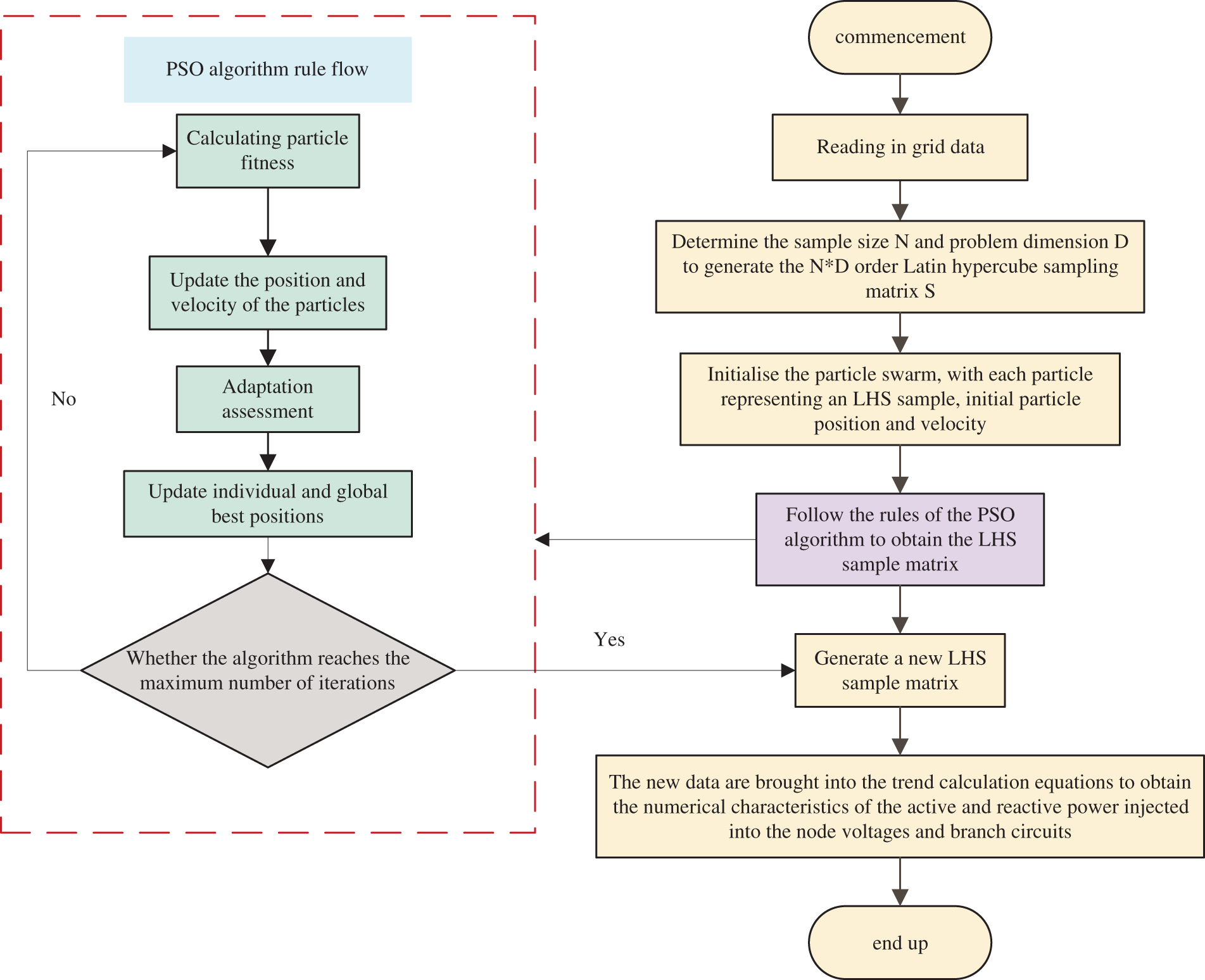
Figure 1: Flowchart of probabilistic tidal current calculation for PSO improved LHS

4  Probabilistic Tidal Current Calculation Based on PSO-LHS

4.1 Input Random Variable Model

4.1.1 Probabilistic Modeling of Wind Power Generation

The Weibull distribution can adapt to various shapes of wind speed distribution curves and accurately fit actual wind speed data, offering a precise depiction of wind speed patterns. Consequently, this paper employs the two-parameter Weibull distribution to model wind speed distribution. Its probability density function is:

f(v)=kc(vc)k−1exp⁡[−(vc)k](5)

In this example, the wind speed is represented by v, the shape parameter by k, and the scale parameter by c, where k=11.8003 and c=4.1416.

The relationship between wind power output active power and wind speed can be described by the following equation:

Pwg={0,v<vI0,v>vOPrv−vinvr−vin,vI<v≤vRPr,vR<v≤vO(6)

where Pr is rated power of the wind farm, vI is cut-in wind speed, vR is rated wind speed and vO is cut-out wind speed; Pr=200 MW, vI=4 m/s, vR=15 m/s, vO=25 m/s. Power factor of 0.95.

4.1.2 Load Probability Model

Loads usually exhibit uncertain characteristics and can generally be represented by a normal distribution:

{f(P)=12πσPexp⁡[−(P−μP)22σP2]f(Q)=12πσQexp⁡[−(P−μQ)22σQ2](7)

where μP and μQ are the average values of active power and reactive power, respectively, σP and σQ are the standard deviations of active power and reactive power, respectively. The normal distribution has a mean of 10% of the expectation and a standard deviation of 10% of the expectation.

4.2 Criteria for Evaluating the Results of Tidal Current Calculations

The validation of the PSO-LHS algorithm is performed by comparing its Probabilistic Load Flow (PLF) results with those obtained from the Latin Hypercube Importance Sampling (LHIS) and Monte Carlo Simulation (MCS) methods. Assuming the accuracy of the PLF results from 10,000 MCS runs, the expected value and standard deviation of the output random variable serve as evaluation criteria. The effectiveness of the PSO-LHS algorithm is then assessed through the relative error in both the expected value and standard deviation.

εμ=|μ−μs||μs|×100%(8)

εσ=|σ−σs||σs|×100%(9)

where μ and σ represent the expected value and standard deviation of the output variables obtained by the method proposed in this paper, while μS and σS represent the baseline expected value and standard deviation of the output random variables. The overall error is evaluated by averaging the relative error of the expected value (ε¯μ) and the relative error of the standard deviation (ε¯σ) averaged over the output random variables at a given node and on a given branch. The overall error is evaluated by averaging the relative error of the expected value (ε¯μ) and the relative error of the standard deviation (ε¯σ) averaged over the output random variables at a given node and on a given branch.

4.3 Setting and Testing of Initial Parameters of PSO-LHS Algorithm

To evaluate the impact of inertia weight and learning factors on the PSO-LHS (Particle Swarm Optimization-Latin Hypercube Sampling) algorithm, this study utilized a two-case experimental design. The first case involved a constant inertia weight with varying learning factors, and the second case involved varying inertia weights with a constant learning factor. The experiments were conducted in a two-dimensional space with a sample size of 30 particles and a maximum of 50 iterations.

1) Firstly, the inertia weight is set to 0.5, and the learning factor is changed to perform sampling, and the sampling results are shown in Fig. 2.

Figure 2: The distribution of the results of the sampling for the four learning factors

Fig. 2 shows that when the inertia weights remain constant while the learning factors are gradually reduced, the distribution graph of the sampling results exhibits minimal variation. This indicates that altering the learning factors has a negligible impact on the PSO-LHS algorithm.

2) Next, the learning factor is set to a constant and the inertia weights are varied to perform the sampling, and the sampling results are shown in Fig. 3.

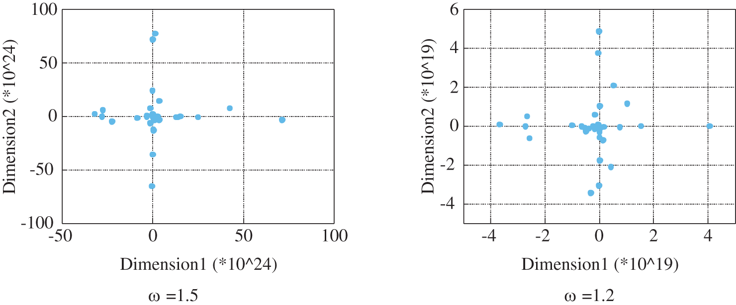
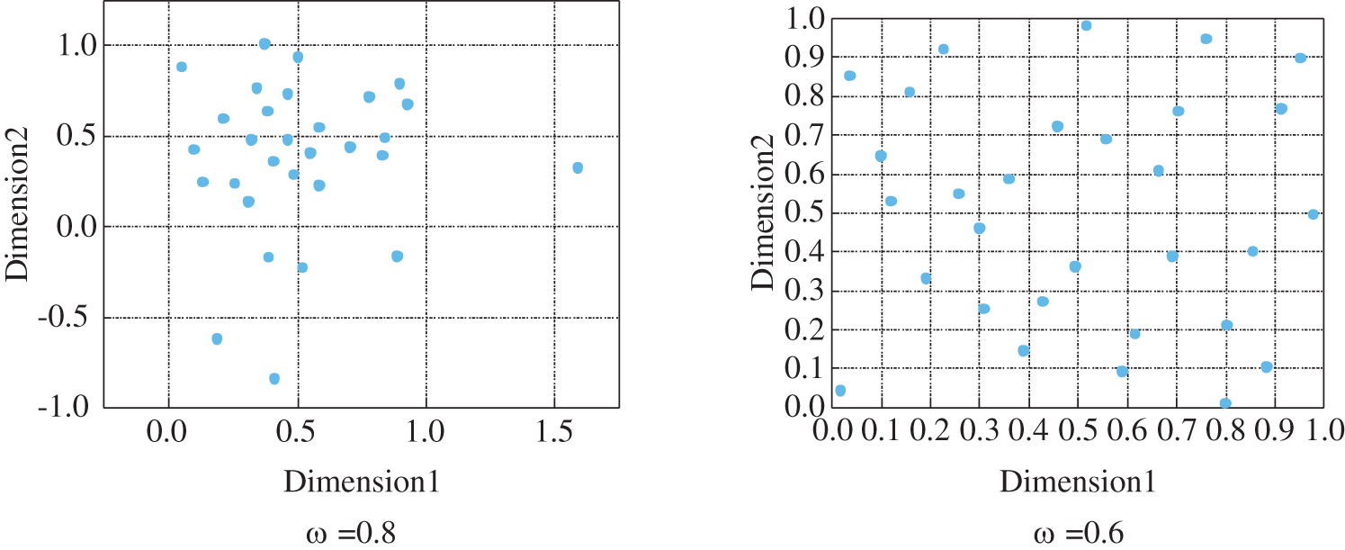
Figure 3: The distribution of the sampling results for the four inertia weights

Fig. 3 shows that when the learning factor is held constant, the sampling distribution graph gradually disperses from concentration as the inertia weight decreases. It can be observed that the inertia weights exert a greater influence on the PSO-LHS algorithm.

Additionally, it was determined that the sampling distribution is most uniform when the inertia weights are reduced to 0.5, and in decreasing order, the distribution gradually transitions from scattered to compact (the distribution plot for ω=0.5 is provided in Section 5.1). In light of the aforementioned sampling outcomes, the PSO algorithm presented in this paper employs a dynamic decreasing strategy based on inertia weights (with an interval of [0.4, 1.5]), and the learning factor is a constant value of 1.5.

5  Algorithm

5.1 IEEE34 Node Simulation Results

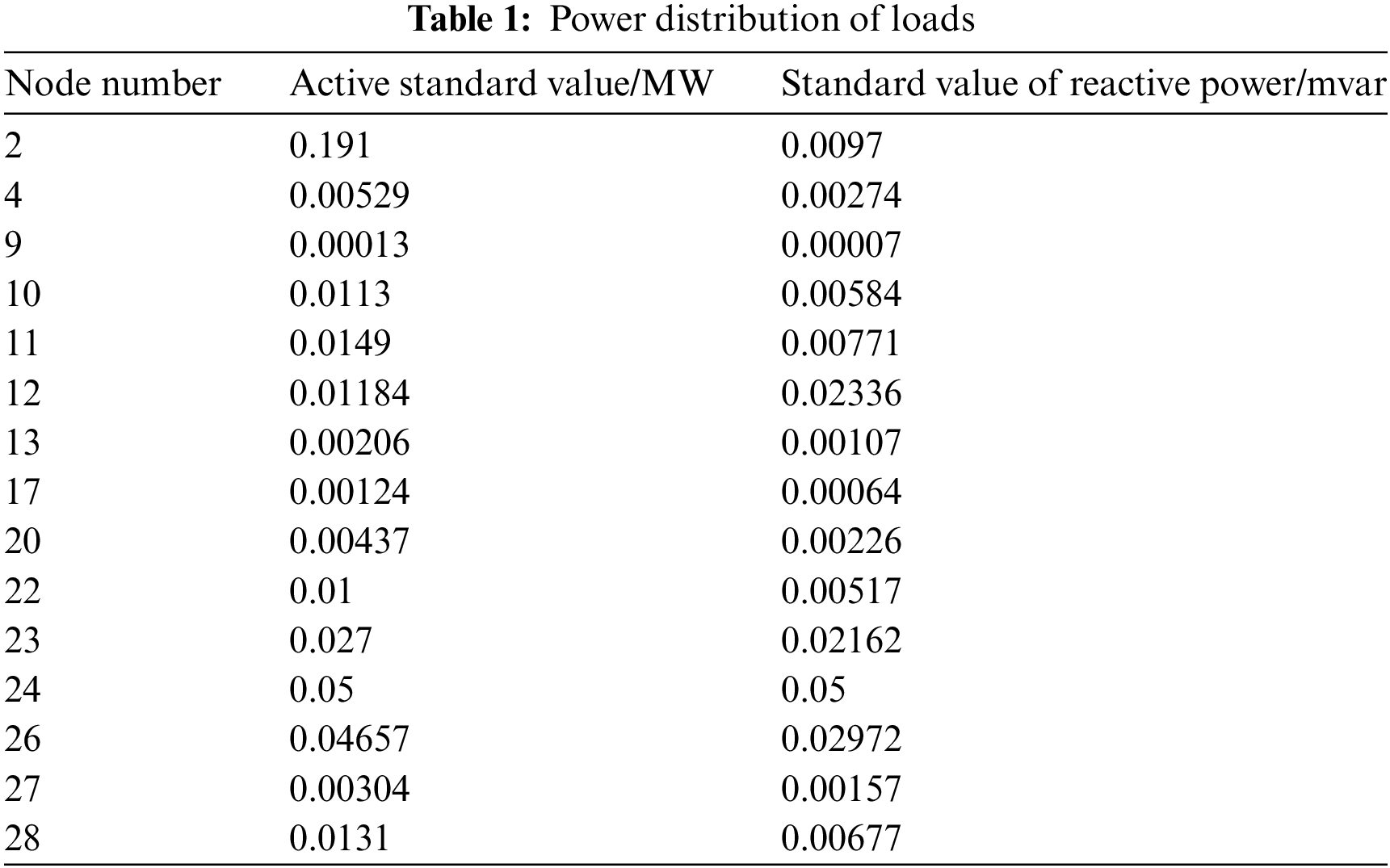
Fig. 4 illustrates the structure of the IEEE34 node system with wind power connected to node 33. The base power value of the system is 100 MVA, the rated power of the wind power is 200 MW, the frequency is 50 Hz.

Figure 4: IEEE34 node system structure diagram

The specific parameters of load active power and load reactive power are shown in Table 1.

The following simulation results can be obtained through simulation:

1) In a two-dimensional space with a total of 30 samples, the PSO-LHS and LHIS algorithms are employed for sampling purposes. The PSO-LHS algorithm utilises an inertia weight of 0.5 and a learning factor of 1.5, resulting in a sampling outcome depicted in Fig. 5.

Figure 5: Sample distribution for the two sampling methods

Fig. 5 shows that the samples generated by PSO-LHS exhibit a more uniform distribution, which effectively reduces the aggregation of sample points and enhances the representativeness of the generated samples.

2) The expected value error and standard deviation of the comparison between the two methods of PSO-LHS and LHIS are shown in Fig. 6.

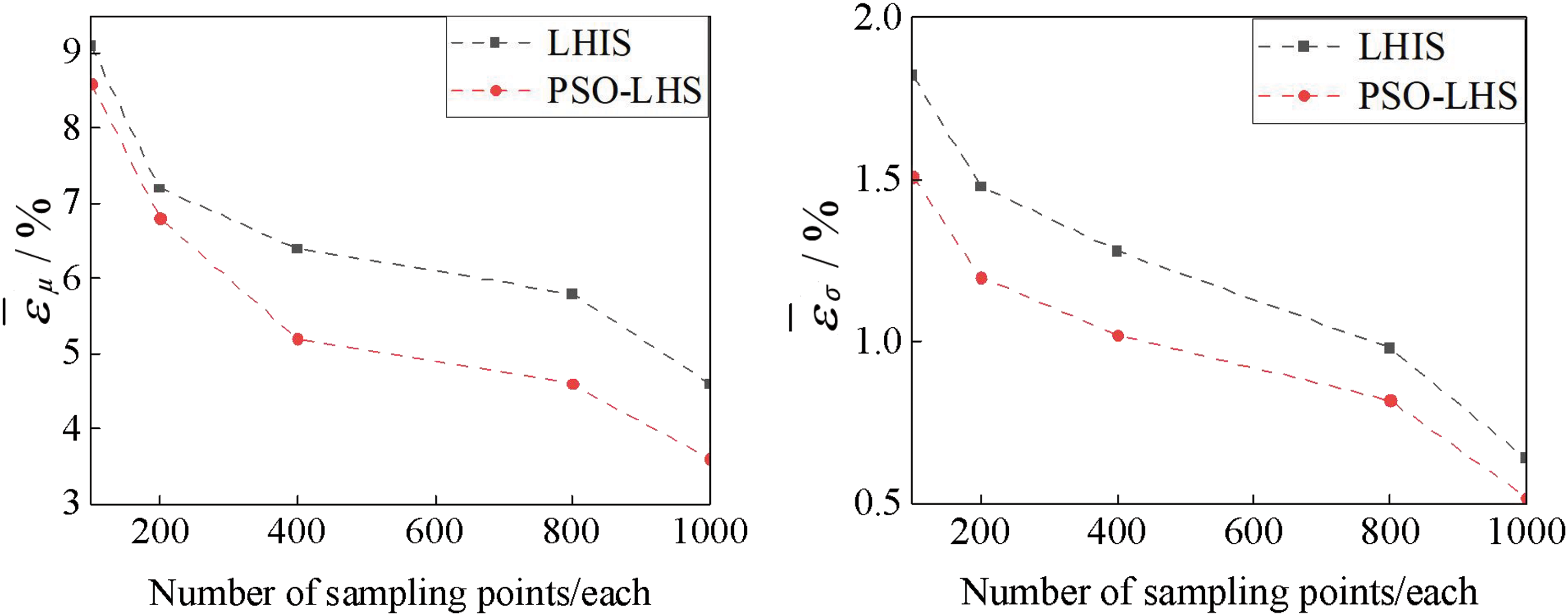
Figure 6: Mean relative error of expected value and standard deviation of voltage amplitude

From Fig. 6, the expectation and standard errors of the output random variables of these two methods are reduced with the increase of the sample size, and it can be seen from Fig. 3 that PSO-LHS can better reduce the error and improve the accuracy for the same sample size.

3) Fig. 7 displays the probability density curves and accumulative distribution curves of the magnitude of the node 33 voltage for sample sizes of 800.

Figure 7: Node 33 voltage probability density curve and cumulative distribution curve

Meanwhile, Figs. 8 and 9 illustrate the probability density curves and cumulative distribution curves of the effective and effective magnitudes of branches 31–33 for sample sizes of 800. Fig. 7 shows that the probabilistic tidal current calculation results of PSO-LHS are similar to the baseline values obtained from 10,000 Monte Carlo calculations.

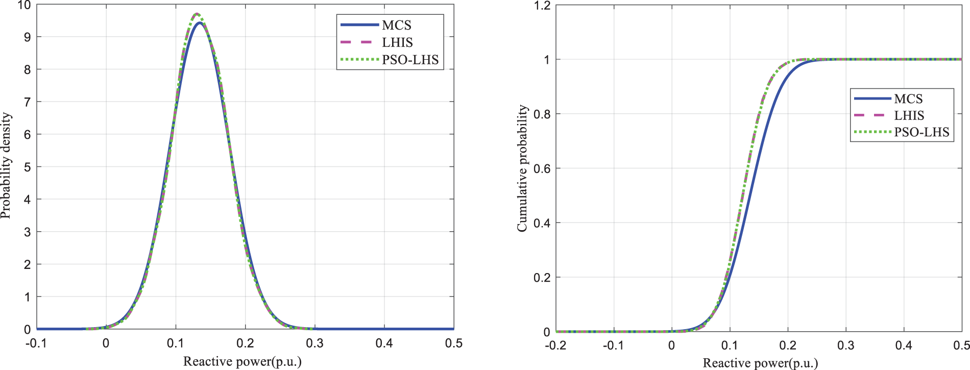
Figure 8: Probability density and cumulative distribution curves for reactive power in branches 31–33

Figure 9: Probability density and cumulative distribution curves for active power on branches 31–33

4) Table 2 presents a comparative time analysis of three methods. Where the computation time of the PSO-LHS algorithm is the average of 100 computation results.

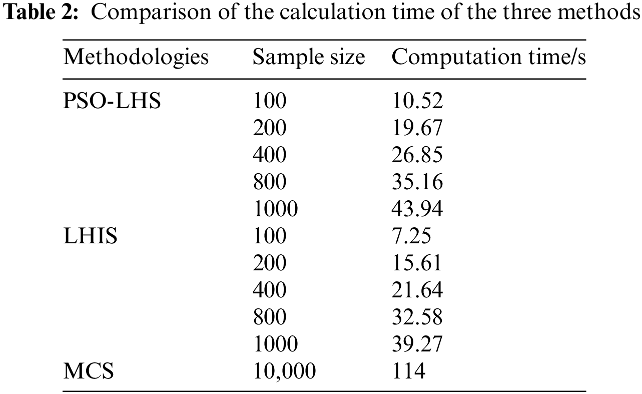
A comparison between the PSO-LHS and LHS algorithms indicates that both exhibit similar execution times. However, the PSO-LHS algorithm converges more slowly due to the additional steps involved in its PSO iterations and optimization search. Despite this slower convergence, the PSO-LHS algorithm demonstrates higher accuracy than the LHS algorithm.

5.2 IEEE118 Node Simulation Results

The validation was conducted using the IEEE118-node system. Furthermore, the results of the probabilistic trend calculations, derived from 10,000 iterations of the Monte Carlo method, were used as a baseline to determine the expected values and standard deviations of the voltages at node 33, the voltages in branches 31–33, and the branch powers. These results were evaluated using average relative errors, as shown in Table 3.

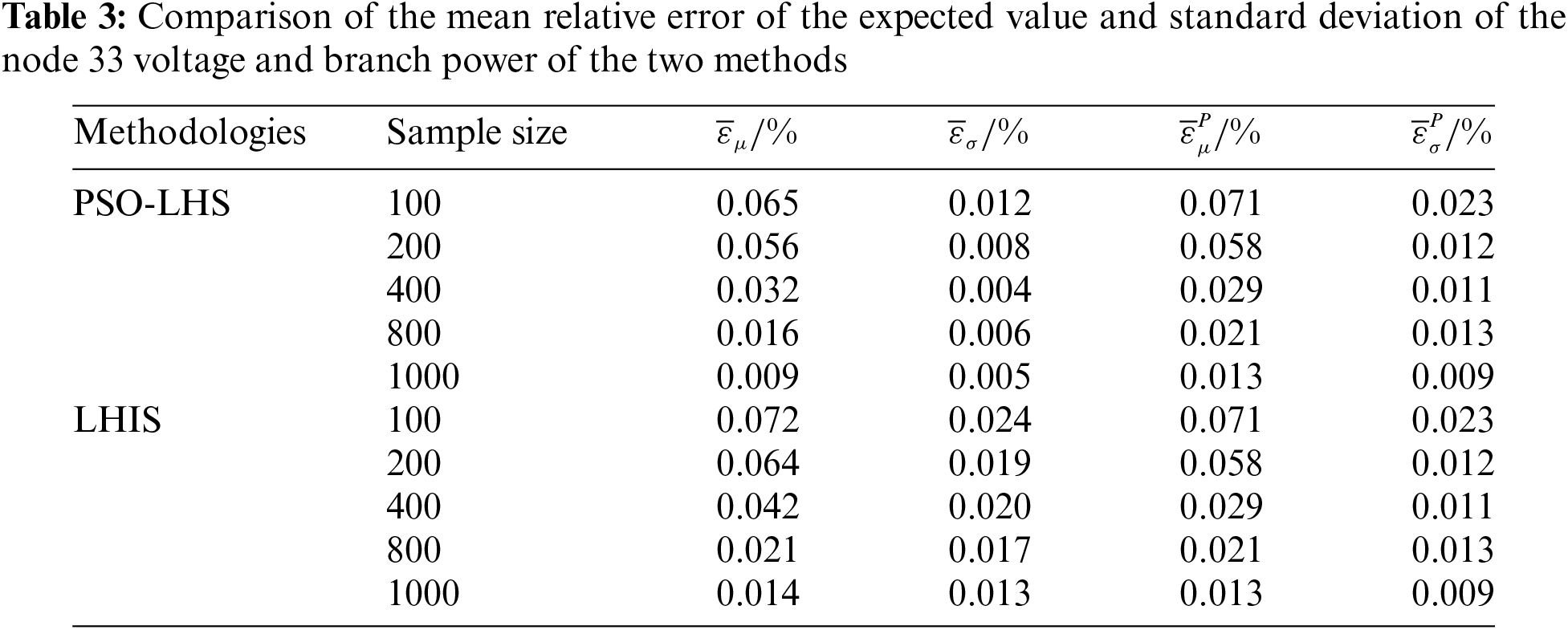
As can be seen in Table 3:

1) Mean Relative Error of Voltage Expectation: The error associated with PSO-LHS is consistently lower than that of LHIS, with a significant reduction as the sample size increases. At a sample size of 1000, PSO-LHS achieves a minimum error of 0.009%, compared to LHIS’s error of 0.014%.

2) Mean Relative Error of Voltage Standard Deviation: Similarly, the error for PSO-LHS is lower than that for LHIS, especially at smaller sample sizes, where the difference is more pronounced. At a sample size of 400, PSO-LHS records the smallest error at 0.004%, while LHIS reports an error of 0.020%.

These findings demonstrate that the PSO-LHS algorithm is consistently more accurate than LHIS, highlighting its superior potential for applications in large-scale node systems.

6  Conclusion

In this paper, we address the issues of long computation time and low computational accuracy in probabilistic trend calculation based on MCS and LHS. We propose an improved method using PSO to enhance LHS, termed PSO-LHS. This method has the following characteristics: (1) PSO-LHS achieves similar accuracy to that obtained by MCS with 10,000 iterations on a small scale, demonstrating its efficiency in reducing the sampling size; (2) Within a sampling range of 100 to 800, PSO-LHS outperforms LHS and MCS in terms of accuracy. Hence, this proposed method is highly suitable for probabilistic tidal current calculations in wind power systems.

Acknowledgement: I would like to thank the editors and the anonymous reviewers for the helpful comments and suggestions that improve the presentation of the manuscript.

Funding Statement: The authors received no specific funding for this study.

Author Contributions: The authors confirm that their contributions to the paper are as follows: research conception and design: Shilin Song, Xingsheng Wang; data collection: Xingsheng Wang; analysis and interpretation of results: Shilin Song, Xingsheng Wang; draft manuscript preparation: Shilin Song. All authors reviewed the results and approved the final version of the manuscript.

Availability of Data and Materials: The data that support the findings of this study are available from the corresponding author upon reasonable request.

Ethics Approval: Not applicable.

Conflicts of Interest: The authors declare that they have no conflicts of interest to report regarding the present study.

References

1. F. Alasali, K. Nusair, H. Foudeh, W. Holderbaum, A. Vinayagam and A. Aziz, “Modern optimal controllers for hybrid active power filter to minimize harmonic distortion,” Electronics, vol. 11, no. 9, Apr. 2022, Art. no. 1453. doi: 10.3390/electronics11091453. [Google Scholar] [CrossRef]

2. B. Borkowska, “Probabilistic load flow,” IEEE Trans. Power Appar. Syst., vol. 93, no. 3, pp. 752–759, May 1974. doi: 10.1109/TPAS.1974.293973. [Google Scholar] [CrossRef]

3. Y. H. Luo, X. Wang, and S. J. Yan, “Risk assessment of photovoltaic distribution network based on adaptive kernel density estimation and cumulant method,” Energy Rep., vol. 8, no. 13, pp. 1152–1159, Nov. 2022. doi: 10.1016/j.egyr.2022.08.156. [Google Scholar] [CrossRef]

4. L. A. Gallego, J. F. Franco, and L. G. Cordero, “A fast-specialized point estimate method for the probabilistic optimal power flow in distribution systems with renewable distributed generation,” Int. J. Electr. Power Energy Syst., vol. 131, Oct. 2021, Art. no. 107049. doi: 10.1016/j.ijepes.2021.107049. [Google Scholar] [CrossRef]

5. Y. F. Sun et al., “Probabilistic load flow calculation of AC/DC hybrid system based on cumulant method,” Int. J. Electr. Power Energy Syst., vol. 139, Jul. 2022, Art. no. 107998. doi: 10.1016/j.ijepes.2022.107998. [Google Scholar] [CrossRef]

6. J. Bogovič and M. Pantoš, “Probabilistic three-phase power flow in a distribution system applying the pseudo-inverse and cumulant method,” J. Electr. Eng., vol. 73, no. 2, pp. 124–131, May 2022. doi: 10.2478/jee-2022-0016. [Google Scholar] [CrossRef]

7. M. Qiao, X. Q. Tong, J. H. Li, and G. Xiong, “Static voltage stability influence evaluation method of distribution network including electric vehicles based on LHS-PPF,” Energy Rep., vol. 9, no. 7, pp. 277–287, Dec. 2023. doi: 10.1016/j.egyr.2023.04.095. [Google Scholar] [CrossRef]

8. I. O. Guimarães, A. M. L. D. Silva, L. C. Nascimento, and F. F. Mahmoud, “Reliability assessment of distribution grids with DG via quasi-sequential Monte Carlo simulation,” Elect. Power Syst. Res., vol. 229, pp. 110122, Apr. 2024. doi: 10.1016/j.epsr.2024.110122. [Google Scholar] [CrossRef]

9. R. H. Kan, Y. C. Xu, Z. H. Li, and L. Mi, “Calculation of probabilistic harmonic power flow based on improved three-point estimation method and maximum entropy as distributed generators access to distribution network,” Elect. Power Syst. Res., vol. 230, May 2024, Art. no. 110197. doi: 10.1016/j.epsr.2024.110197. [Google Scholar] [CrossRef]

10. T. Yang, Z. N. Yang, F. Li, and H. Y. Wang, “A short-term wind power forecasting method based on multivariate signal decomposition and variable selection,” Appl. Energy, vol. 360, Apr. 2024, Art. no. 122759. doi: 10.1016/j.apenergy.2024.122759. [Google Scholar] [CrossRef]

11. L. D. A. Takara, A. C. Teixeira, H. Yazdanpanah, V. C. Mariani, and L. D. S. Coelho, “Optimizing multi-step wind power forecasting: Integrating advanced deep neural networks with stacking-based probabilistic learning,” Appl. Energy, vol. 369, Sep. 2024, Art. no. 123487. doi: 10.1016/j.apenergy.2024.123487. [Google Scholar] [CrossRef]

12. H. Fatoorehchi and M. Ehrhardt, “A combined method for stability analysis of linear time invariant control systems based on Hermite-Fujiwara matrix and Cholesky decomposition,” Can. J. Chem. Eng., vol. 101, no. 12, pp. 7043–7052, Dec. 2023. doi: 10.1002/cjce.24962. [Google Scholar] [CrossRef]

13. D. E. Huntington and C. S. Lyrintzis, “Improvements to and limitations of Latin hypercube sampling,” Probab. Eng. Mech., vol. 13, no. 4, pp. 245–253, Oct. 1998. doi: 10.1016/S0266-8920(97)00013-1. [Google Scholar] [CrossRef]

14. S. Bhardwaj, S. Raghuraman, J. B. Yerrapragada, and A. Jagirdar, “Low-complex and low-power n-dimensional gram-schmidt orthogonalization architecture design methodology,” Circuits Syst. Signal Process, vol. 41, pp. 1633–1659, Sep. 2021. doi: 10.1007/s00034-021-01852-0. [Google Scholar] [CrossRef]

15. Q. Y. Kenny, W. Li, and A. Sudjianto, “Algorithmic construction of optimal symmetric Latin hypercube designs,” J. Stat. Plan. Inference, vol. 90, no. 1, pp. 145–159, Sep. 2000. doi: 10.1016/S0378-3758(00)00105-1. [Google Scholar] [CrossRef]

16. R. Xiong et al., “Improved cooperative competitive particle swarm optimization and nonlinear coefficient temperature decreasing simulated annealing-back propagation methods for state of health estimation of energy storage batteries,” Energy, vol. 292, Apr. 2024, Art. no. 130594. doi: 10.1016/j.energy.2024.130594. [Google Scholar] [CrossRef]

17. R. H. Bonsa, D. W. Abraham, and A. W. Getachew, “Printing PEDOT: PSS optimized using response surface method (RSM) and genetic algorithm (GA) via modified 3D printer for perovskite solar cell applications,” Appl. Mater. Today, vol. 37, Apr. 2024, Art. no. 102134. doi: 10.1016/j.apmt.2024.102134. [Google Scholar] [CrossRef]

18. Y. L. Zhao, P. Chen, R. K. Zhou, P. Luo, and Y. X. Dong, “An improved LHS for probabilistic power flow calculation method considering non-positive definite correlation,” (in Chinese), Zhejiang Electr. Power, vol. 39, no. 4, pp. 36–42, Apr. 2020. doi: 10.19585/j.zjdl.202004006. [Google Scholar] [CrossRef]

19. Q. Li, X. Wang, and S. Rong, “Probabilistic load flow method based on modified Latin hypercube-important sampling,” Energies, vol. 11, no. 11, Nov. 2018, Art. no. 3171. doi: 10.3390/en11113171. [Google Scholar] [CrossRef]

20. X. T. Xia and L. Y. Xiao, “Probabilistic power flow method for hybrid AC/DC grids considering correlation among uncertainty variables,” Energies, vol. 16, no. 6, Mar. 2023, Art. no. 2547. doi: 10.3390/en16062547. [Google Scholar] [CrossRef]

21. P. Zhang, H. Zhang, Y. F. Li, W. Chen, X. Y. Zhang and H. J. Li, “Probabilistic power flow calculation using semi invariant method based on improved LHS,” (in Chinese), Acta Energiae Solaris Sinica, vol. 42, no. 1, pp. 14–20, Jan. 2021. doi: 10.19912/j.0254-0096.tynxb.2018-0705. [Google Scholar] [CrossRef]

22. B. Zhou, X. Yang, D. Yang, Z. Yang, T. Littler and H. Li, “Probabilistic load flow algorithm of distribution networks with distributed generators and electric vehicles integration,” Energies, vol. 12, no. 22, Nov. 2019, Art. no. 4234. doi: 10.3390/en12224234. [Google Scholar] [CrossRef]

23. M. Badi and S. Mahapatra, “Optimal reactive power management through a hybrid BOA-GWO–PSO algorithm for alleviating congestion,” Int. J. Syst. Assur. Eng. Manage., vol. 14, pp. 1437–1456, Jun. 2023. doi: 10.1007/s13198-023-01946-9. [Google Scholar] [CrossRef]