Seasonal Short-Term Load Forecasting for Power Systems Based on Modal Decomposition and Feature-Fusion Multi-Algorithm Hybrid Neural Network Model

1  Introduction

Accurate and effective short-term load forecasting is essential to ensure the safe and reliable operation of the power system and serves as the foundation for the strategic planning of power generation within the grid. The demand for higher precision in short-term power load forecasting has increased with the implementation of electricity market reforms. In recent years, frequent occurrences of extreme weather, severe natural disasters, and other exceptional events have heightened the challenges of power load forecasting. Factors such as seasonality, abrupt meteorological changes, and holidays significantly impact forecasting accuracy, particularly during periods of extreme weather and transitional phases. These fluctuations in forecasting accuracy pose a serious threat to the secure functioning of the power grid. Hence, in the context of climate change, it is crucial to accurately understand the correlation and sensitivity changes between electricity load and temperature. This understanding enables the prediction of the proportion of electricity load in each season, ensuring the normal operation and scheduling control of electricity post-climate change.

Traditional methods [1–3] combined with machine learning [4–7] for short-term electric load forecasting offer speed advantages but often overlook sample temporal relationships [8]. Deep learning models have become prevalent in this field owing to their ability to address both temporal and nonlinear issues through specialized recurrent units such as recurrent neural network (RNN), long short-term memory (LSTM) networks, and gated recurrent unit (GRU). Among these, RNNs demonstrate greater effectiveness than feedforward neural networks. However, training RNNs presents challenges owing to issues such as gradient disappearance arising from time series complexities, resulting in less optimal prediction outcomes [9]. LSTM mitigates the problem of gradient disappearance in RNNs by enhancing their recurrent units [10]. Studies [11,12] have utilized LSTM for short-term load prediction and demonstrated its capability to enhance prediction accuracy compared with existing methods. However, incorporating reverse information often proves beneficial in bolstering the model’s predictive power. By integrating past operation outcomes with the current process, forward information fulfills the role of “considering the above information” [13]. Studies have investigated the application of bidirectional long short-term memory (BiLSTM) networks for load prediction [14,15] and have revealed the superior ability of the networks for representing continuous time series compared with LSTM.

In real-world scenarios, electric loads are influenced by customer energy usage patterns and are heavily impacted by seasonal and meteorological factors such as temperature, wind speed, and date type. Additionally, the integration of numerous energy storage devices and distributed renewable power sources into the grid, alongside the adoption of demand-side management policies incentivized by tariffs, further complicates load forecasting. Employing a single approach for load forecasting becomes challenging owing to these diverse influences. To address this challenge, electric load forecasting employs hybrid forecasting approaches that integrate data preprocessing techniques with current forecasting models. This hybrid approach enables better accommodation of external factors and enhances prediction accuracy. The literature [16] enhanced the accuracy of short-term electricity load forecasting through a multidimensional feature extraction framework. However, the complexity of the model and its dependence on high-quality data could potentially affect the balance between forecasting time and accuracy. Another study [17] introduced a two-stage intelligent feature engineering (IFE) and serial multi-timescale forecasting framework, aiming to balance the stability of load trend forecasting with the accuracy of load fluctuation detail forecasting. However, there may be redundancies in feature inputs. Another study [18] presented a short-term load forecasting model that combined empirical mode decomposition (EMD) with LSTM. This model divides the load into several components, allowing each to be treated independently to mitigate interference among different temporal features. However, EMD is susceptible to a confounding modal problem, which can impact prediction accuracy. Another study [19] employed ensemble empirical mode decomposition (EEMD) to further decompose these components, aiming to reduce the influence of strong non-stationary components generated by wavelet packet decomposition on the prediction. However, EEMD introduces noise, and the increased number of components resulting from both decompositions could significantly increase the time required for prediction by neural networks. Another study [20] employed an LSTM neural network to forecast wind speed sequences following the application of variational mode decomposition (VMD) and break them down into several intrinsic mode functions (IMFs). However, VMD has the drawback that all components may not align consistently with the original sequence after reconstruction. Studies [21,22] have employed complete ensemble empirical mode decomposition with adaptive noise (CEEMDAN) combined with LSTM to mitigate nonlinear features through the decomposition of the load sequence into multiple modal components. Furthermore, a previous study proposed the use of the improved complete ensemble empirical modal decomposition with adaptive noise (ICEEMDAN) method [23] to enhance the CEEMDAN algorithm. This new algorithm defines the IMF as the difference between the current value of the residual signal and its local mean, and it extracts IMF values by introducing specific white noise. Compared with previous techniques, ICEEMDAN successfully enhances noise reduction impact by addressing potential residual noise and spurious patterns in the eigenmodal function of the CEEMDAN model.

Various conditions, such as severe weather and special events, can significantly impact power consumption, leading to the occurrence of abnormal data in time series. In the analysis of factors affecting electricity load, determining which features to use plays a crucial role in load prediction accuracy; thus, feature analysis and neural network models are required. Commonly used feature analysis methods include the covariance method, Pearson coefficient method, maximal information coefficient (MIC) method, and MIC-based max-relevance and min-redundancy (mRMR) algorithm [24]. The Pearson coefficient approach and the covariance method can assess the linear relationship between sequences. Energy coupling involves many nonlinear relationships, and linearly describing users’ energy demand is challenging. Therefore, for addressing nonlinear relationships, methods such as the MIC method and the mRMR method are more suitable. In one study [25], the MIC method was applied to short-term electricity price forecasting, and the screening efficiency of feature sequences was effectively improved. However, this method did not consider the high redundancy of feature sequences in the system. mRMR, a filtered feature selection method, can incorporate redundancy in sequences into the screening indicator, making it more suitable for systems with high redundancy. Moreover, mRMR stands out from other filtering algorithms for its ability to maximize differences between features while filtering out the most relevant features related to categorical variables, so that the optimal feature combination is obtained. In load forecasting, mRMR can extract the most relevant and smallest possible subset of elements influencing load power variation.

The aforementioned studies exhibit several deficiencies. First, electric load exhibits clear seasonal characteristics, with different regions experiencing varied load distributions across the four seasons. Therefore, relying solely on continuous load data as the training set without considering seasonal variations may compromise load forecasting accuracy in power systems. In contrast, utilizing a seasonal training set to train neural networks can notably enhance prediction accuracy compared with approaches neglecting seasonal variations. However, studies considering seasonal training sets for power load prediction are scarce. Second, power load is significantly influenced by temperature and humidity data, with varying impacts across different seasons and dates. The accuracy of the model’s forecasts may be affected when a single prediction model is used for historical power load. Hence, utilizing data preprocessing methods that encompass a comprehensive analysis of seasonal features is crucial. These features can then be integrated into the hybrid forecasting approach of current forecasting models.

Drawing from the above analysis and existing algorithms, this paper proposes a seasonal short-term load combination prediction model for power systems. The model is based on modal decomposition and feature fusion within a multi-algorithm hybrid neural network framework. This approach aims to address the challenge of poor prediction accuracy caused by external factors. The proposed method fully considers the seasonal variations in load characteristics. The method departs from the traditional approach of training models on continuous datasets and instead uses load data from the same season as the prediction season adopted for model training. This approach aims to enhance prediction accuracy and relevance. First, a time-frequency analysis is conducted for each of the four seasons. ICEEMDAN is then applied to decompose the load data for each season, and a new sequence is derived through the reconstruction of each decomposition component according to the refined composite multiscale fuzzy entropy (RCMFE) value in entropy theory. Second, considering the regional variations in seasonal impacts on load power, the correlation between electric load and influencing factors representing seasonal variations (such as temperature, humidity, and rainfall) is analyzed. Subsequently, a subset of features showing a strong correlation with the load is selected through the mRMR method. Data processing, combined with seasonal feature analysis, forms the set of variable input features for the prediction model. The BiLSTM model is employed to separately predict different load components across various seasons. Hyperparameter tuning is conducted using the Bayesian optimization algorithm. The aforementioned process aims to reduce the complexity of the forecasting task while substantially enhancing forecasting accuracy. This improvement enhances the model’s adaptability and precision in forecasting.

2  Algorithm Model Principles

2.1 Characterization of Load Curve Based on Seasonal Characteristics

The power load curve inherently exhibits daily and seasonal cycle characteristics. Specifically, the seasonal pattern of the curve varies, with noticeable differences in peak-to-valley ratios among different regions. Moreover, the load rates and peak-to-valley points vary significantly across seasons. Therefore, the uniform treatment of loads from different seasons affects load prediction accuracy, posing a challenge for traditional short-term load prediction methods. Fig. 1 illustrates the annual load data for a southern region of China, depicting pronounced peak and valley features and substantial fluctuations. Load variation also correlates with seasonal changes and external factors such as weather conditions. For instance, higher temperatures in summer lead to significantly elevated loads compared with other seasons. Additionally, the date type also plays a significant role in load variation. For instance, in areas with large factories, load variations can be substantial depending on whether the day is a double holiday. Moreover, holidays significantly impact load characteristics. As depicted in Fig. 1, a noticeable drop in load occurs during the Spring Festival in winter and the National Day in autumn. In summary, mining the load change patterns under specific meteorological conditions from extensive meteorological load data allows for the utilization of seasonal change information and enhances prediction performance. Additionally, accurately quantifying the influence of meteorological factors on load under complex weather conditions is crucial for improving prediction accuracy.

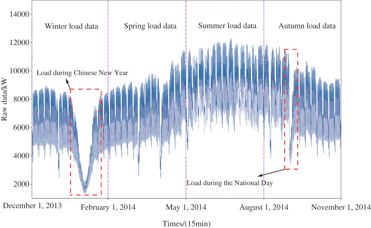
Figure 1: Original load data

2.2 Modal Decomposition and Sequence Aggregation Based on Seasonal Features

2.2.1 ICEEMDAN

In this research, the ICEEMDAN method is employed to decompose the yearly load into four seasons and various IMFs and a residual, ranging from high to low frequency, according to the time scale of the load series. At different time scales, each IMF accurately represents the distinct elements of the electric load without interference. During the decomposition process, the ICEEMDAN algorithm ensures frequency continuity between neighboring scales by incorporating white noise ηi(t) and local averaging. This adaptive decomposition effectively breaks down the non-stationary sequence x(t) into a finite number of IMF components with varying frequency characteristics and a residual component, thereby mitigating the load’s nonlinear characteristics and refining load analysis [26]. The decomposition steps of ICEEMDAN are illustrated in Eq. (1).

xi(t)=x(t)+α0E1(ηi(t))rk(t)=⟨M(rk−1(t)+αk−1Ek(ηi(t)))⟩IMFk(t)=rk−1(t)−rk(t)(1)

where xi(t) is the noise-added signal; x(t) is the original load sequence; Ek(⋅) represents the kth-order modal obtained by the EMD algorithm; ηi(t) represents the addition of the ith white noise; rk(t) denotes the kth-order residual component; ⟨⋅⟩ represents the mean calculation; M(⋅) represents envelope calculation; αk−1=βk−1std(x(t))/std(Ek(wi(t))) represents the standard deviation of white noise for noise removal. βk denotes the inverse of the expected signal-to-noise ratio between the noise-added and analyzed signals. std denotes the standard deviation; IMFk(t) represents the kth-order modal component.

2.2.2 Subsequence Aggregation Based on RCMFE

The combined electric load forecasting model, which integrates decomposition methods, significantly enhances all evaluation indices. However, as the number of decomposition levels increases, the computational complexity and time consumption of the combined model increase exponentially. To achieve a balance between forecasting performance and time cost, this paper adopts the RCMFE algorithm proposed in the literature [27] to aggregate the subseries divided and decomposed separately for each of the four seasons.

The compound multiscale fuzzy entropy (CMFE) and multiscale fuzzy entropy (MFE) form the basis of the enhanced method known as RCMFE. MFE serves as a time series complexity measurement algorithm. However, owing to the reduction in the length of coarse-grained sequences as the scale factor increases, MFE may encounter issues with erroneous entropy values. CMFE aims to improve the accuracy of MFE but does not resolve the problem of undefined entropy [28]. The RCMFE method addresses the limitations of both CMFE and MFE by aggregating all coarse-grained sequences under a scale factor τ before computing their fuzzy entropy, thereby minimizing the occurrence of undefined entropy values in CMFE. Eq. (2) presents the calculation formulas for CMFE and RCMFE applied to the electricity load of a specific season.

yk,j(τ)=1τ∑i=(j−1)τ+kjτ+k−1xjCMFE(x,τ,m,n,r)=1τ∑k=1τFuzzyen(yk(τ),m,n,r)RCMFE(x,τ,m,n,r)=−ln⁡(∑k=1τN¯k,τm+1∑k=1τN¯k,τm)(2)

where x={x1,x2,…,xN} is the load power time series. The coarse-grained sequence is called. yk,j(τ)={yk,1(τ),yk,2(τ),…,yk,p(τ)}, 1≤k≤τ, 1≤j≤N/τ. m denotes the embedding dimension; n denotes the fuzzy function gradient; r denotes the similarity tolerance; N¯k,τm+1(n,r) and N¯k,τm(n,r) are the number of matching vector pairs calculated for the kth coarse-grained sequence under the scale factor τ, respectively; N¯k,τm+1=1τ∑k=1τNk,τm+1; and N¯k,τm=1τ∑k=1τNk,τm. According to the CMFE calculation results, when the coarse-grained sequence in the CMFE calculation is too short owing to a specific scale, the CMFE value becomes undefined. Consequently, the likelihood of encountering undefined entropy values increases during the calculation of short sequences, imposing limitations on CMFE. Undefined entropy exists in RCMFE only when all Nk,τm+1 and Nk,τm are zero. Hence, the RCMFE method effectively reduces the likelihood of encountering undefined entropy in applications involving short coarse-grained sequences, in contrast to the CMFE technique. This enhancement contributes to improved accuracy in entropy estimation.

2.3 Correlation Analysis of Load-Influencing Factors Based on Seasonal Characteristics

Given the uncertainty associated with weather factors across all seasons and the challenge of acquiring complete instantaneous data, conducting correlation analysis and extracting features from both power load and weather factors are necessary. This approach allows for an analysis of the interaction between power load and weather and facilitates the effective selection of input features for the prediction model. Considering that both loads and influencing factors exhibit strong nonlinearity, this paper employs the mRMR feature extraction algorithm proposed in the literature. This algorithm is utilized to extract features from historical electric load power, weather data, and calendar rules for each season (spring, summer, autumn, and winter). These features are then filtered to identify the most relevant seasonal factors affecting load changes across all seasons, serving as input data for power prediction.

mRMR is a filtered feature selection method capable of identifying a subset of features with the highest correlation and lowest redundancy. Its evaluation function considers both feature–category and feature–feature correlations. The feature screening calculation procedure is outlined in Eq. (3). The technique utilizes mutual information to estimate the correlation between variables.

I(X;Y)=∬p(x,y)log⁡p(x,y)p(x)p(y)dxdy{maxD(S,P),D=1|S|∑fi∈SI(fi,P)minR(S),R=1|S|2∑fi,fj∈SI(fi,fj)maxJ(D,R),J=D−Rmaxfi=S−St−1[I(fi,c)−1t−1∑fi∈st−1I(fi,fj)](3)

where p(x),p(y) are the marginal probability functions of the relevant variables, p(x,y) is the joint probability distribution, and Xand Y are two characteristic variables. The average of all mutual information values between each factor set fi and P serves as the basis for determining the correlation of the factor set of load power P. The highest correlation between features and categories and the lowest level of feature redundancy are denoted by the letters maxD(S,P) and minR(S), respectively. S denotes the feature set; fi denotes the ith feature; P denotes the target category; I(fi,fj) and I(fi,P) respectively denote the mutual information between features i and j and between features i and the target category P. The tth feature is then chosen from the set S−St−1 once the feature selection algorithm’s evaluation function maxJ(D,R) has been applied. Maximizing the difference between univariate correlation and redundancy results in the addition of the tth feature.

2.4 Load Forecasting Methods

In this study, we integrate data processing with seasonal feature analysis to address significant variations in electric demand across the four seasons. These combined techniques constitute the variable input features for the prediction model. To enhance the network’s forecasting accuracy and adaptability, the BiLSTM model is employed to separately predict each component of the load for each of the four seasons. Subsequently, the Bayesian optimization algorithm finetunes the model’s hyperparameters before the application of the model to seasonal short-term load forecasting in the power system.

2.4.1 BiLSTM

To tackle the issue of gradient vanishing inherent in the RNN structure, the LSTM model is commonly employed in models aimed at enhancing RNN performance. The LSTM model structure incorporates a cell state connection and addresses the gradient vanishing problem by introducing gating cells and linear connections to capture longer time dependencies. The specific structure of the LSTM is illustrated in Fig. 2.

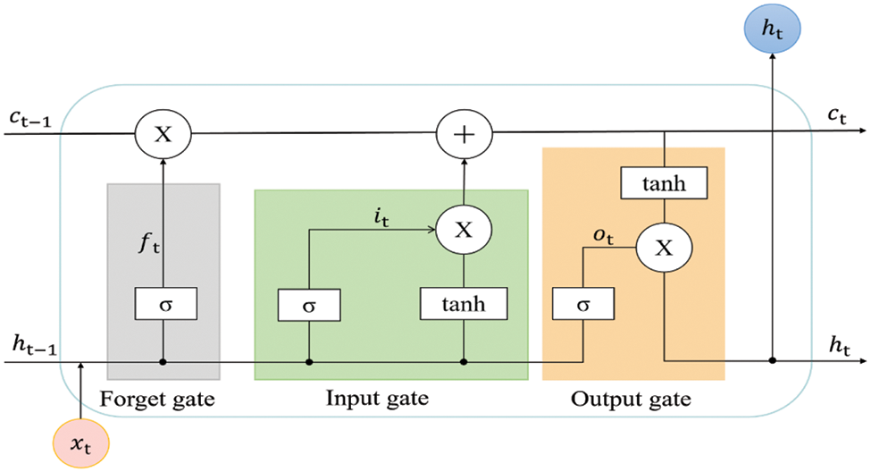
Figure 2: Structure of LSTM

The LSTM network consists of two channels and three gating units: a forgetting unit ft, an input unit it, and an output unit ot, The lower channel serves as a short-term memory channel for retaining short-term information ht, while the upper channel functions as a long-term memory channel for storing long-term memory information ct. Information addition and discarding are managed by the three gating units. Eq. (4) is employed for data transfer.

{ft=σ(Wf[ht−1,xt]+bf)it=σ(Wi[ht−1,xt]+bi)ct′=tanh⁡(Wc[ht−1,xt]+bc)ot=σ(Wo[ht−1,xt]+bo)ct=ft∗ct−1+it∗ct′ht=ot∗tanh⁡(ct)yt=ht(4)

where σ(⋅) denotes the Sigmoid activation function; W denotes the weight matrix; xt denotes the current input vector; and bf, bi, bc, and bo denote the corresponding bias terms of the forgetting cell, the input cell, the cell state, and the output gate, respectively. The previous moment’s output ht−1 is obtained through the combination of the current moment hidden layer output ht with the current moment’s long-term memory state ct and the information ot from the output gate output, resulting in the predicted power at moment t.

Owing to the evident forward and backward regularities in load sequences, LSTM models can only utilize historical information from the forward sequence, resulting in a phase lag during the prediction of fluctuation processes. Hence, the impacts of both historical and future loads on prediction accuracy are considered in load prediction. The BiLSTM neural network comprises two LSTM neural networks in forward and reverse directions. Different from traditional LSTM models, the BiLSTM neural network accounts for both forward and backward data regularities [29]. The neural network generates predictions from two historical and future directions using two independent networks. The BiLSTM structure enables bidirectional temporal feature extraction from input data, thereby enhancing global and comprehensive temporal feature extraction.

2.4.2 BiLSTM Hyperparametric Optimization Based on Bayesian Optimization

Selecting hyperparameters for neural networks is challenging and can lead to underfitting or overfitting, necessitating hyperparameter optimization. Current widely used swarm intelligence algorithms, such as particle swarm and sparrow algorithms, require initializing the optimization function and continually updating the initialization matrix. This process involves numerous calls to the neural network during training, which significantly increases the cost of training the optimization-seeking model. Consequently, swarm optimization approaches are not well-suited for hyperparameter optimization in deep learning models. In this study, the hyperparameter optimization problem of BiLSTM models is addressed through the Bayesian optimization approach.

The Bayesian optimization method selects the next most promising sample point according to the posterior distribution of the objective function. The method uses evaluation data from earlier functions based on the Bayes theorem. The posterior probability distribution is derived by observing the prior probability of the hyperparameters using a probabilistic surrogate model. The next optimal hyperparameter evaluation point is then determined by employing an acquisition function and the posterior probability distribution. The fundamentals of this algorithm are outlined in the literature [30]. Fig. 3 illustrates the hyperparameter optimization procedure of the prediction model.

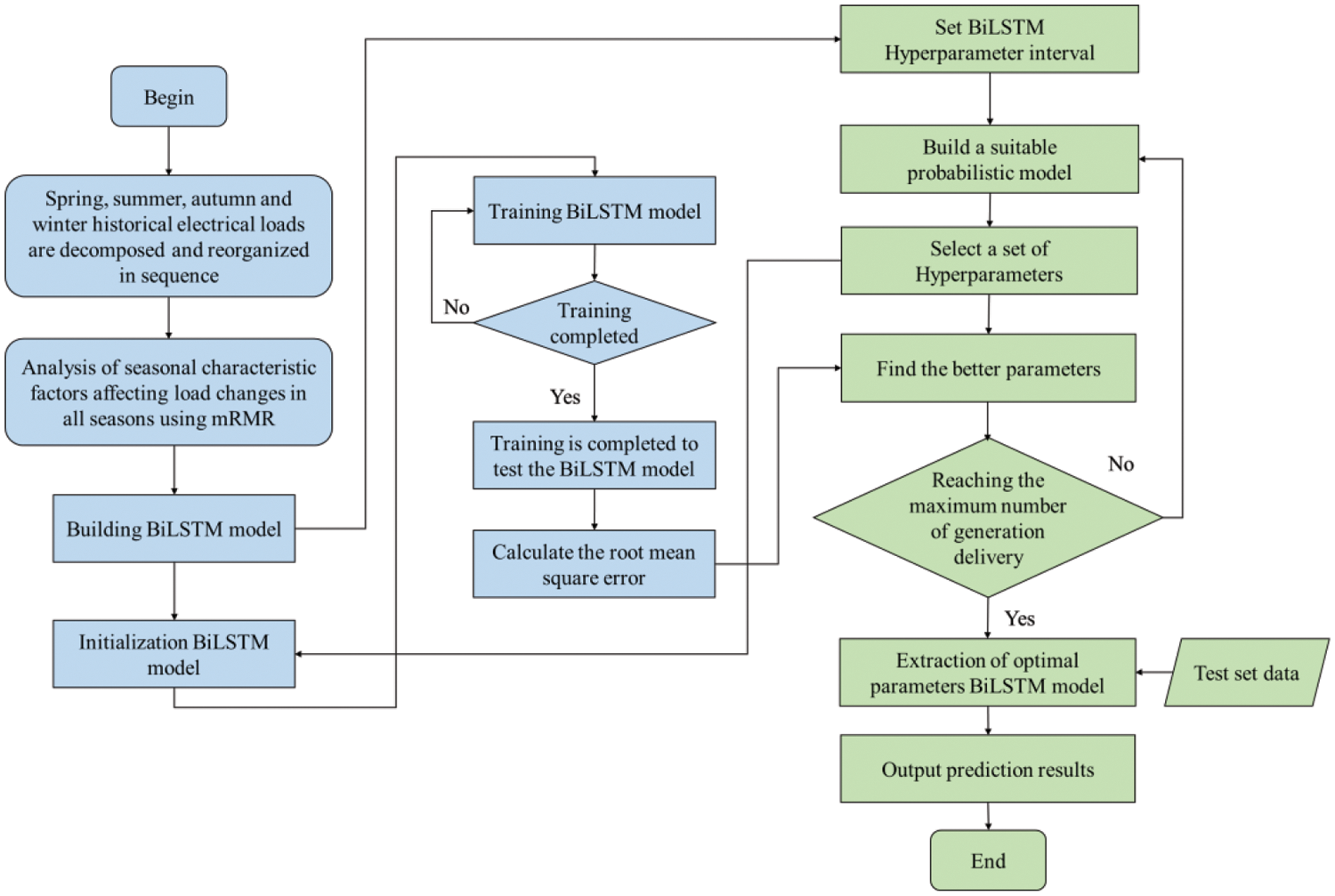
Figure 3: BiLSTM hyperparameter search flow chart based on Bayesian optimization

2.4.3 Data Preprocessing

Considering the variations in magnitudes among different influencing factors and historical load data across all seasons, directly using them as input features may impact the prediction accuracy of the model. In this study, raw data are scaled using the min–max normalization approach, as shown in Eq. (5).

x′=x−xminxmax−xmin(5)

where the original, normalized, and original data’s maximum and minimum values are represented by x, x′, and xmax, and xmin, respectively.

3  Seasonal Short-Term Load Combination Forecasting Model for a Power System Based on Modal Decomposition and Feature-Fusion Multi-Algorithm Hybrid Neural Network

This paper proposes a seasonal short-term load combination forecasting model (ICEEMDAN-RCMFE-mRMR-Bayes-BiLSTM [IRMBB]) based on modal decomposition and feature fusion within a multi-algorithm hybrid neural network. The model combines the time-frequency analysis method, entropy theory, and deep learning algorithm to fully account for the seasonal change characteristics of power system load. The overall framework of the model is illustrated in Fig. 4.

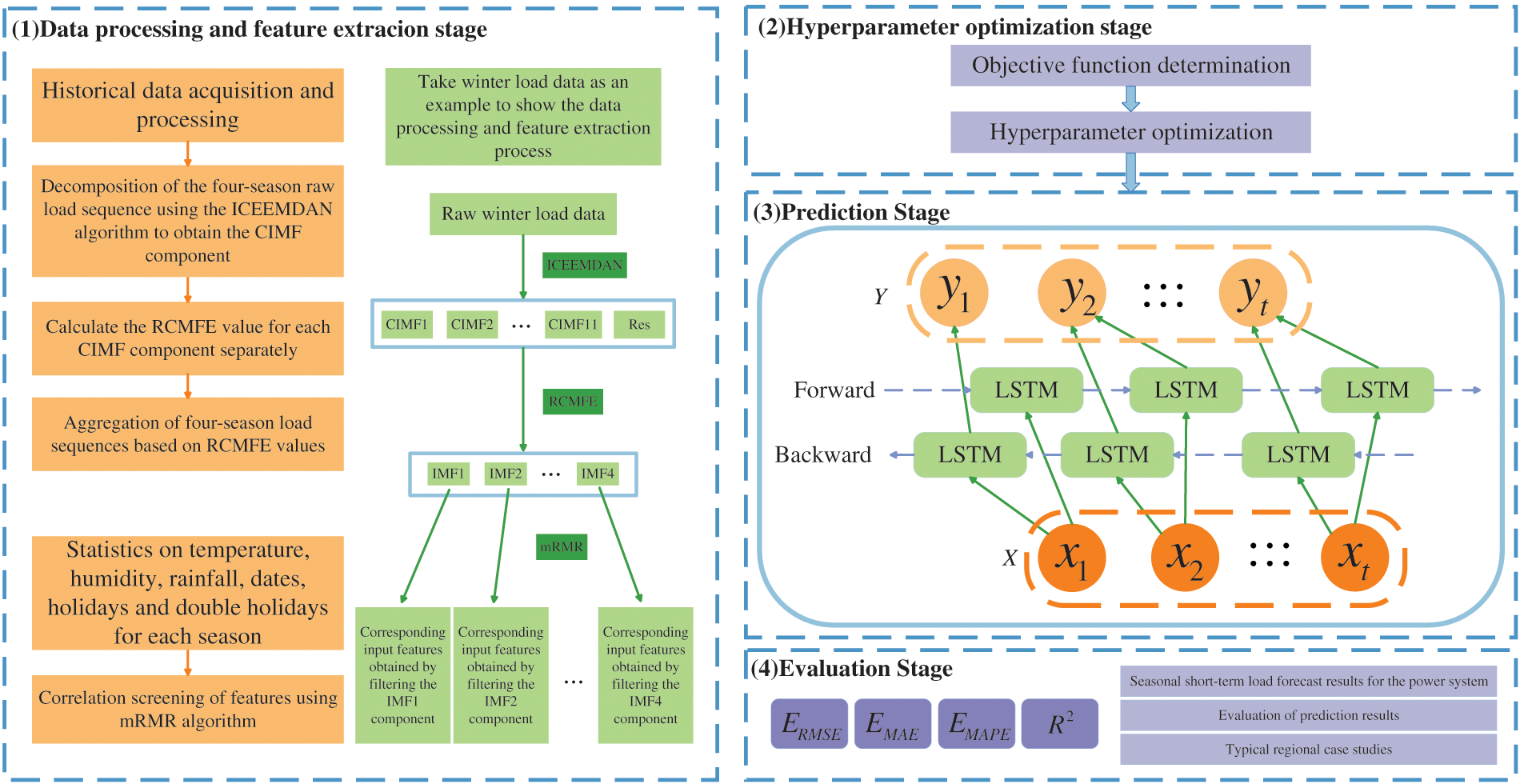
Figure 4: Overall framework of load forecasting model

3.1 Modal Decomposition and Complexity Assessment of Raw Load Data

In this paper, a dataset spanning 12 months, from December 2013 to November 2014, for a southern region of China is selected as experimental data. This dataset includes load data, date types, meteorological factors, and other relevant data, with a sampling interval of 15 min. The 12 months of data are divided into four quarters: December 2013 to February 2014 (winter), March to May 2014 (spring), June to August 2014 (summer), and September to November 2014 (autumn).

The subseries aggregation process based on RCMFE is illustrated in Fig. 5. First, modal decomposition of the raw load data for different seasons is conducted using ICEEMDAN. After several iterations, the parameter settings for the ICEEMDAN decomposition of the winter load are finalized. The standard noise deviation is set to 0.5, the average number of iterations for the signal is 500, and the maximum number of iterations is set to 2000. Twelve components, including residuals, are obtained after load decomposition for all four seasons, as depicted in Fig. 5a. After the CIMF components are obtained, the RCMFE values of different components in different seasons are calculated through the RCMFE method. The magnitude of these values reflects the complexity of the data, in which larger values indicate higher complexity and stronger nonlinearity. The RCMFE parameters are set as follows: the embedding dimension is 2, the gradient of the fuzzy function is 2, and the similarity tolerance is 0.15. The RCMFE values of each component of the four-season load are obtained, as shown in Fig. 5b. For different seasons, according to the purple division line in Fig. 5b, CIMF components with similar complexity are grouped into the same class and merged into a smaller number of IMF components (Fig. 5c). The specific merging results are presented in Table 1.

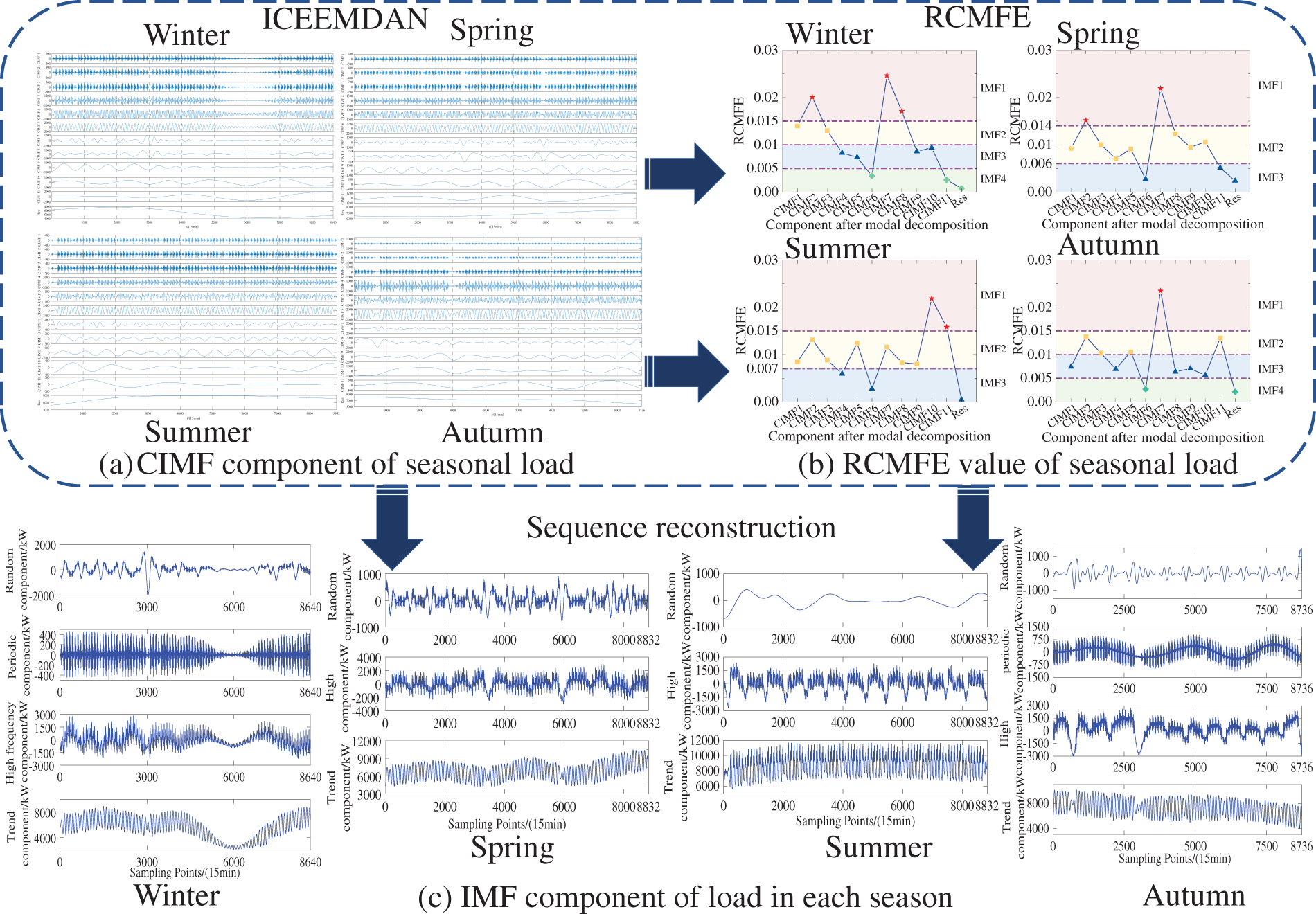
Figure 5: Subsequence aggregation process based on RCMFE: (a) CIMF component of seasonal load; (b) RCMFE value of seasonal load; (c) IMF component of load in each season

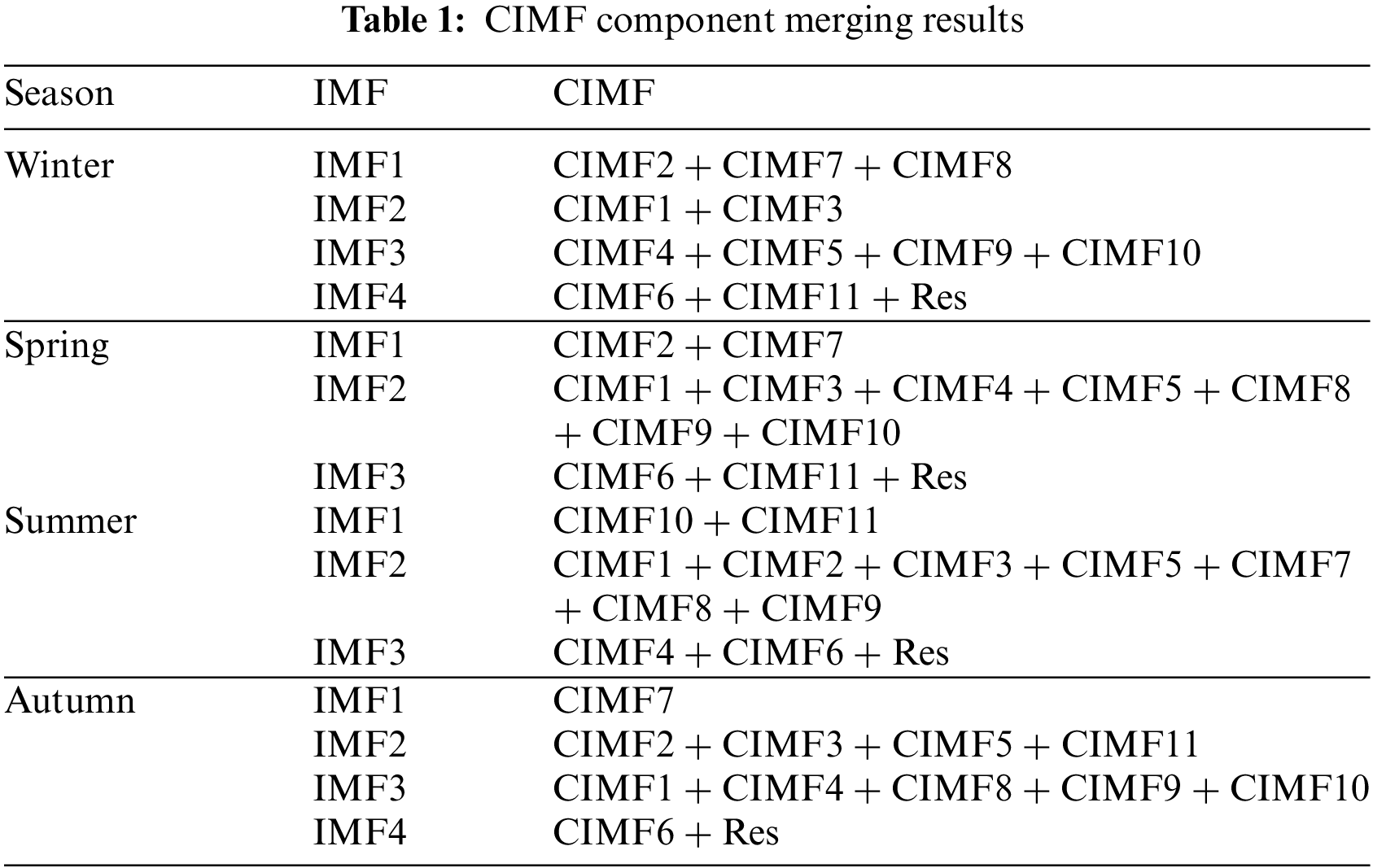
As depicted in Fig. 5a, the decomposed components of each seasonal load exhibit distinct modal patterns without evident overlap, significantly reducing the original data’s non-smoothness. The low-frequency components exhibit clear trends and smoothness, while the high-frequency components display notable periodicity. The regularity of each component is more apparent than in the original data, as highlighted by the CIMF component assignment results in Table 1. Combining the CIMF components of spring and summer loads yields three IMF components, while the CIMF components of winter and autumn loads result in four IMF components, including the random component IMF1, characterized by high complexity and irregularity. The periodic component IMF2 exhibits small amplitude, high frequency, and distinct periodicity. This high-frequency component comprises CIMF components with higher frequencies, exhibiting poor regularity and RCMFE values with a range of [0.005,0.01]. The component features gentle fluctuations. The trend component IMF4 demonstrates clearer regularity and reflects the overall change of the original load data to some extent. The component generally appears smoother and more regular than the original load data in each season.

3.2 Correlation Analysis and Feature Screening of Load-Influencing Factors

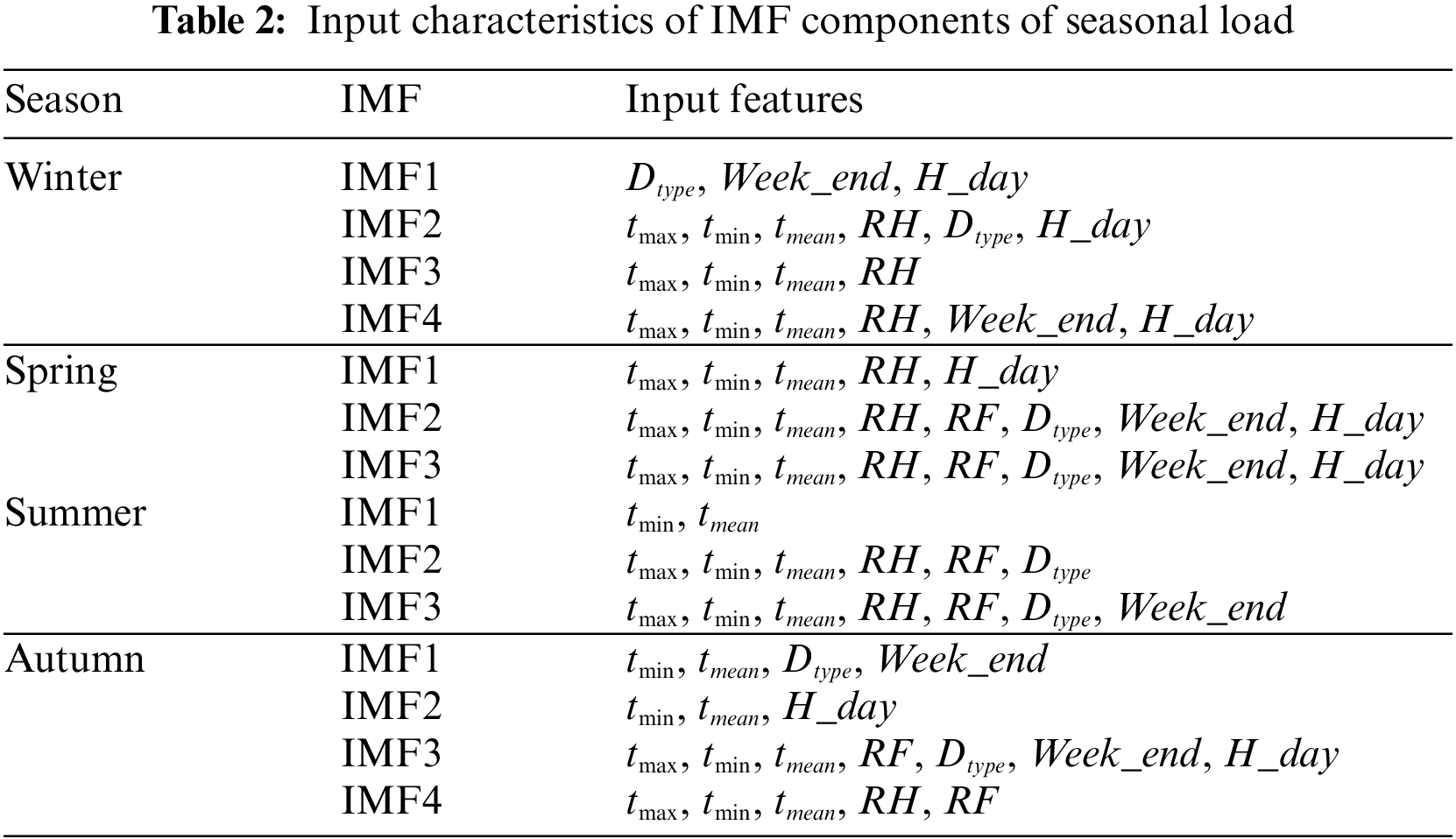
Owing to significant variations in meteorological conditions from season to season, customers’ electricity consumption behavior varies considerably, thereby impacting load changes. In addition to the historical load feature of each component, this paper selects the maximum temperature tmax(°C), minimum temperature tmin(°C), average temperature tmean(°C), relative humidity RH(%), rainfall RF(mm), and weekday Dtype (expressed by 1–7). The eight influencing factors considered as input features are related to whether the day is a holiday H_day (coded as 1 for yes, 0 for no) or a double holiday Week_end (coded as 1 for yes, 0 for no).

In this study, the mRMR approach is utilized to assess the strength of the association between the IMF components of each seasonal load and the features based on the IMF components derived from different seasonal loads. The magnitude of the correlation between each seasonal load and the input features to be selected is shown in Fig. 6.

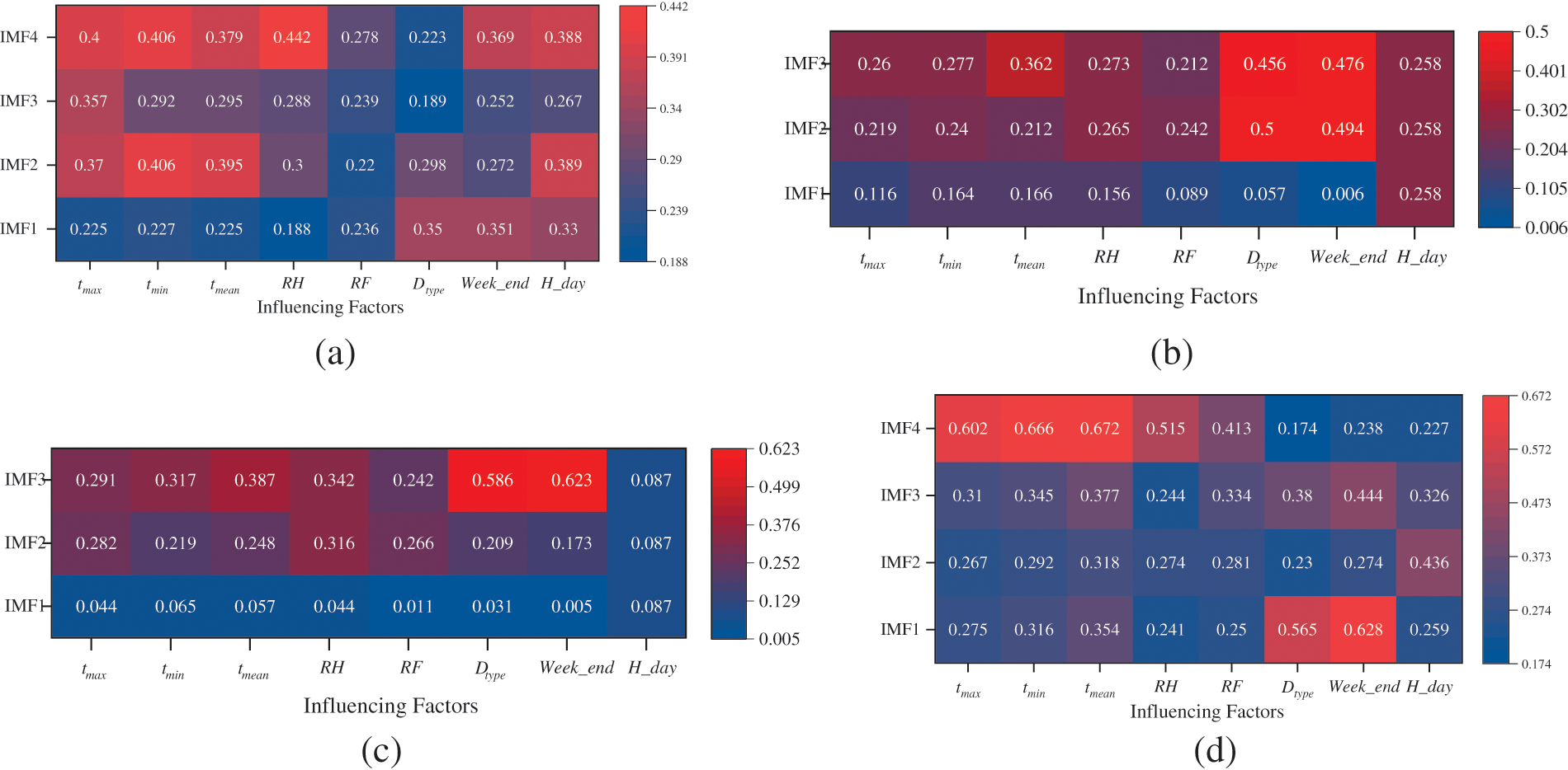
Figure 6: Size of seasonal loads correlated with influencing factors: (a) size of winter loads correlated with influencing factors; (b) size of spring loads correlated with influencing factors; (c) size of summer loads correlated with influencing factors; (d) size of fall loads correlated with influencing factors

As depicted in Fig. 6, significant differences in correlation magnitude between various IMF components and influencing factors are evident. For instance, as shown in Fig. 6a, the IMF1 component shows stronger correlation with three date type factors, Dtype, Week_end, and H_day; hence, these factors are selected as input features in addition to the historical load data from 24 h ago. Similarly, for the IMF3 component, four meteorological conditions tmax, tmin, tmean, and RH exhibit stronger influence, leading to their inclusion as additional input features. The IMF2 and IMF4 components exhibit a stronger correlation with each other; thus, these four influencing factors are considered for inclusion. In the case of the IMF3 component, tmax, tmin, tmean, and RH, which are the four meteorological condition factors that have a greater influence on the component, are taken as additional input features. For the IMF2 and IMF4 components, their correlations with certain meteorological factors and date-type factors are notable, warranting the inclusion of most features except for those with weaker correlations, the rest of the features should be chosen into the input feature set. Table 2 presents the best-selected input features for the IMF components of each seasonal load, excluding historical load data. These features are selected to ensure the quality of input features while reducing the forecasting model’s burden.

After completing the feature screening, this paper employs the BiLSTM model based on the Bayesian optimization algorithm to train the selected key feature subsets. The bidirectional learning structure of the model ensures comprehensive and consistent feature extraction, enhancing the model’s ability to capture temporal dynamics in the data. This approach improves the accuracy and reliability of the model in complex time series analysis.

3.3 Hyperparameter Optimization

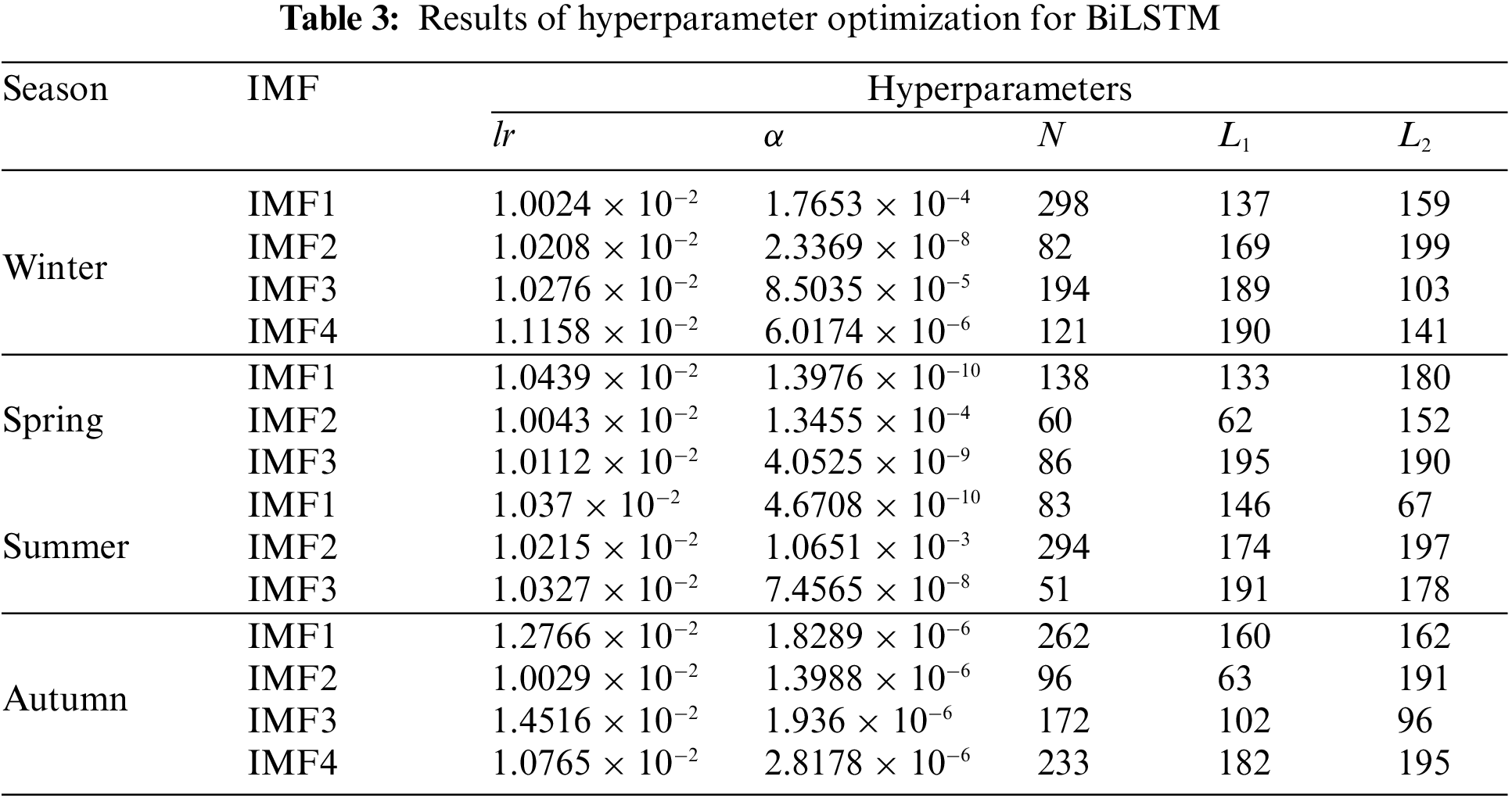
The trial-and-error approach is a conventional strategy for optimization searching. Given the significant subjectivity and unpredictability of human parameter adjustment and the substantial number of components to be forecasted, this study employs the sliding window approach for prediction. Following data normalization, the Bayesian optimization technique is utilized to tune the five hyperparameters of the BiLSTM network: learning rate lr, L2 regularization coefficient α, the maximum amount of iterations N, and the number of neurons in the first and second hidden layers L1 and L2, respectively. The optimization range of BiLSTM is set as follows: the optimization range of learning rate lr is [10−6, 0.1], the optimization range of L2 regularization coefficient α is [10−10, 10−2], the optimization domain for the maximum number of iterations N is [50, 300], while the domain for the number of neurons in the first and second hidden layers L1 and L2 is [20, 200]. The Adam optimizer is used for training, and the BiLSTM batch sample size is 256. Table 3 displays the final optimization findings.

3.4 Evaluation Metrics

The average absolute error EMAE, root mean square error ERMSE, average absolute percentage error EMAPE, and the coefficient of determination R2 are utilized as assessment indices to evaluate the prediction performance of the model developed in this study. Among these, EMAE represent the model’s real error level; ERMSE indicate the impact of extreme outliers on prediction outcomes; EMAPE represent the average of the absolute percentage error sum of load values, which assesses the overall effectiveness of the prediction model; and R2 evaluates the goodness-of-fit of the prediction model. The expressions for each evaluation index are as follows:

EMAE=1n∑i=1n|y^i−yi|ERMSE=1n∑i=1n(y^i−yi)2EMAPE=1n∑i=1n|y^i−yiyi|×100%R2=1−∑i=1n(y^i−yi)2∑i=1n(yi−y¯)2(6)

where y^i, yi, and y¯ are the averages of the predicted, true, and real values, respectively.

4  Example Analysis

The technique described in this paper is implemented using MATLAB 2021a. The computer’s specifications are as follows: an NVIDIA RTX2060 graphics card, an Intel Core i5-10200H CPU operating at 2.40 GHz, and 16 GB of RAM. The data preceding the last week of load for each season are used as training data. Single-step predictions of load for the last week of each season are separately conducted using a sliding window approach. The sliding window length is set to 96, meaning that the first 96 sets of samples are used as input data, the 97th sampling point is predicted, and then the sliding window is shifted. The 97th data point obtained from the prediction is used as a new feature to achieve rolling prediction. As described in Section 4.1, this paper employs multiple methods considering seasonal change information, and the IRMBB method is proposed to conduct experiments on a dataset for a city in Southern China. Furthermore, a comparative analysis is conducted to validate the effectiveness of the combined forecasting method proposed in this paper for efficient load forecasting. As described in Section 4.2, methods considering seasonal change information and those not considering it are employed to predict extremely high and extremely low weekly loads in Texas, USA. Weekly loads during extreme high and low temperatures are forecasted using both methods. A comparative analysis is conducted to verify the effectiveness of considering seasonal variation information in improving load prediction accuracy.

4.1 Comparative Analysis of Different Combination Forecasting Models

4.1.1 Balancing Prediction Accuracy and Time Effectiveness

To verify the superiority of the seasonal short-term load combination prediction model proposed in this paper, the author compares the proposed ICEEMDAN-RCMFE-mRMR-Bayes-BiLSTM (IRMBB) model with three previously reported models: ICEEMDAN-mRMR-Bayes-BiLSTM (IMBB) [31], mRMR-Bayes-BiLSTM (MBB) [32], and ICEEMDAN-RCMFE-mRMR-SSA-BiLSTM (IRMSB) [33]. To ensure fairness in the comparative analysis, the number of iterations for both Bayesian optimization and sparrow search algorithm (SSA) is set to 30. The population size for SSA is set to 10, with a ratio of 7:2:1 for discoverers, joiners, and alerts in the populations. Fig. 7 shows the prediction time and prediction evaluation index values for the four methods for load prediction across the four seasons.

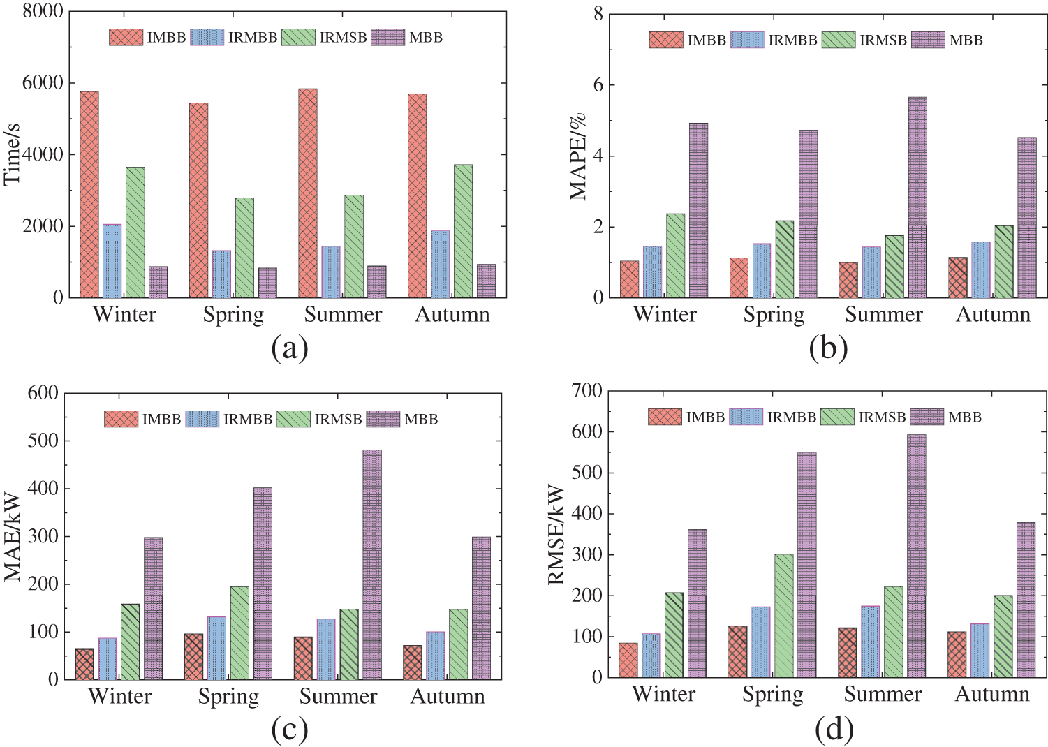
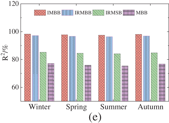
Figure 7: Time spent and evaluation metrics for different models to predict load for various quarters: (a) comparison of time spent; (b) comparison of EMAPE; (c) comparison of EMAE; (d) comparison of ERMSE; (e) comparison of R2

As depicted in Fig. 7a, IMBB spends significantly more time predicting load for each season than IRMBB and MBB. Specifically, the prediction time of IMBB for the spring and summer seasons is over three times that of IRMBB, while for the winter and autumn seasons, the prediction time is over four times that of IRMBB. Conversely, the prediction times of IRMSB for winter, spring, summer, and fall loads are 1.77, 2.1, 1.98, and 1.99 times those of IRMBB, respectively. While both IRMSB and IRMBB predict the same IMF components, the use of the swarm intelligence algorithm SSA to optimize the BiLSTM prediction model in IRMSB, along with a higher dimensionality of training data and larger dataset, contributes to the increased time required for IRMSB’s load prediction. Additionally, BiLSTM requires more hyperparameters for optimization. According to Fig. 7b–e, MBB takes a short time but fails to achieve satisfactory prediction results, because it does not utilize the ICEEMDAN-RCMFE method to process the original load data; instead, it solely relies on Bayes-BiLSTM to predict seasonal load after feature screening. Consequently, its evaluation index values are significantly worse than those of IRMBB proposed in this paper. While IMBB exhibits a better prediction effect than IRMBB, the former consumes too much time, making it inefficient. Although IRMSB exhibits a longer prediction time than IRMBB, the prediction effect of the former is not improved, and the indexes are slightly lower than those of IRMBB. Overall, the superiority of the proposed IRMBB method is verified.

The evaluation values of the four methods across four seasons are presented in Table 4 after the minimization of the “time spent on prediction” index to more quantitatively analyze the proposed method’s superiority in balancing prediction accuracy and prediction time. The author employs the entropy-based TOPSIS (technique for order of preference by similarity to an ideal solution) method [34] to evaluate the four methods described in this section.

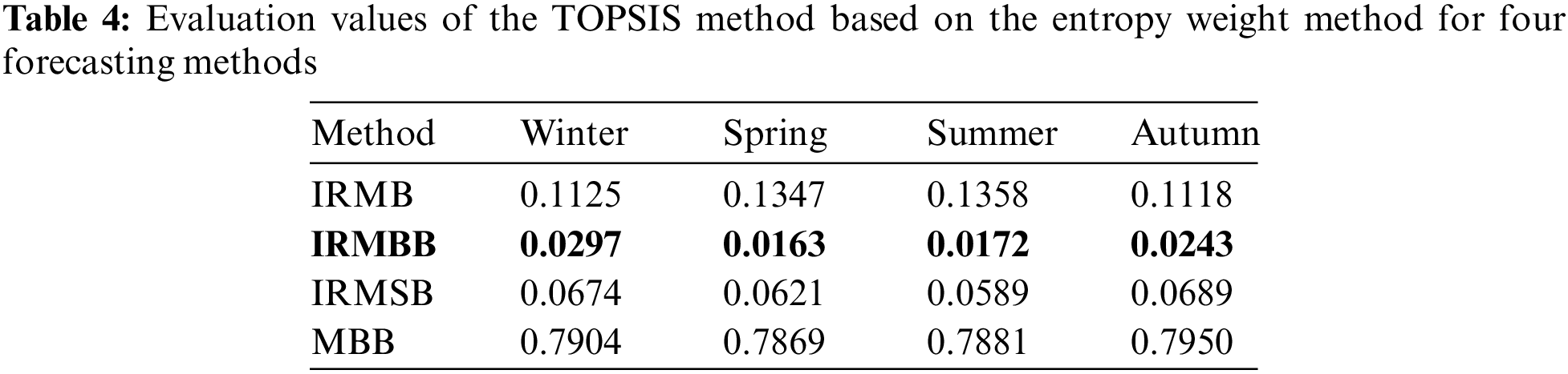
Table 4 reveals that the TOPSIS value for the IRMBB method is the lowest across all four seasons, indicating superior performance. Following closely is the IRMSB method, which exhibits comparable effectiveness to IRMBB in each season, albeit slightly lower. Next is the IRMB method, with the MBB method displaying the highest value and thus the least favorable prediction outcome. Overall, the IRMBB method demonstrates its effectiveness and superiority in achieving a balance between prediction accuracy and prediction time for load forecasting.

4.1.2 Validity of Prediction Accuracy

In this study, five sets of comparison models are constructed to further demonstrate the superiority of the suggested strategy over other combination models in prediction accuracy. The models include: (1) ICEEMDAN-RCMFE-mRMR-BiLSTM (IRMB) [35]; (2) ICEEMDAN-RCMFE-mRMR-Bayes-SVM (IRMBS) [36]; (3) ICEEMDAN-RCMFE-mRMR-Bayes-XGBoost (IRMBX) [37]; (4) ICEEMDAN-RCMFE-mRMR-Bayes-LSTM (IRMBL) [37]; and (5) ICEEMDAN-RCMFE-mRMR-Bayes-GRU (IRMBG) [38]. Table 5 presents the evaluation index values for the predictions of IRMBB as indicated in this study and those of the five sets of comparator models.

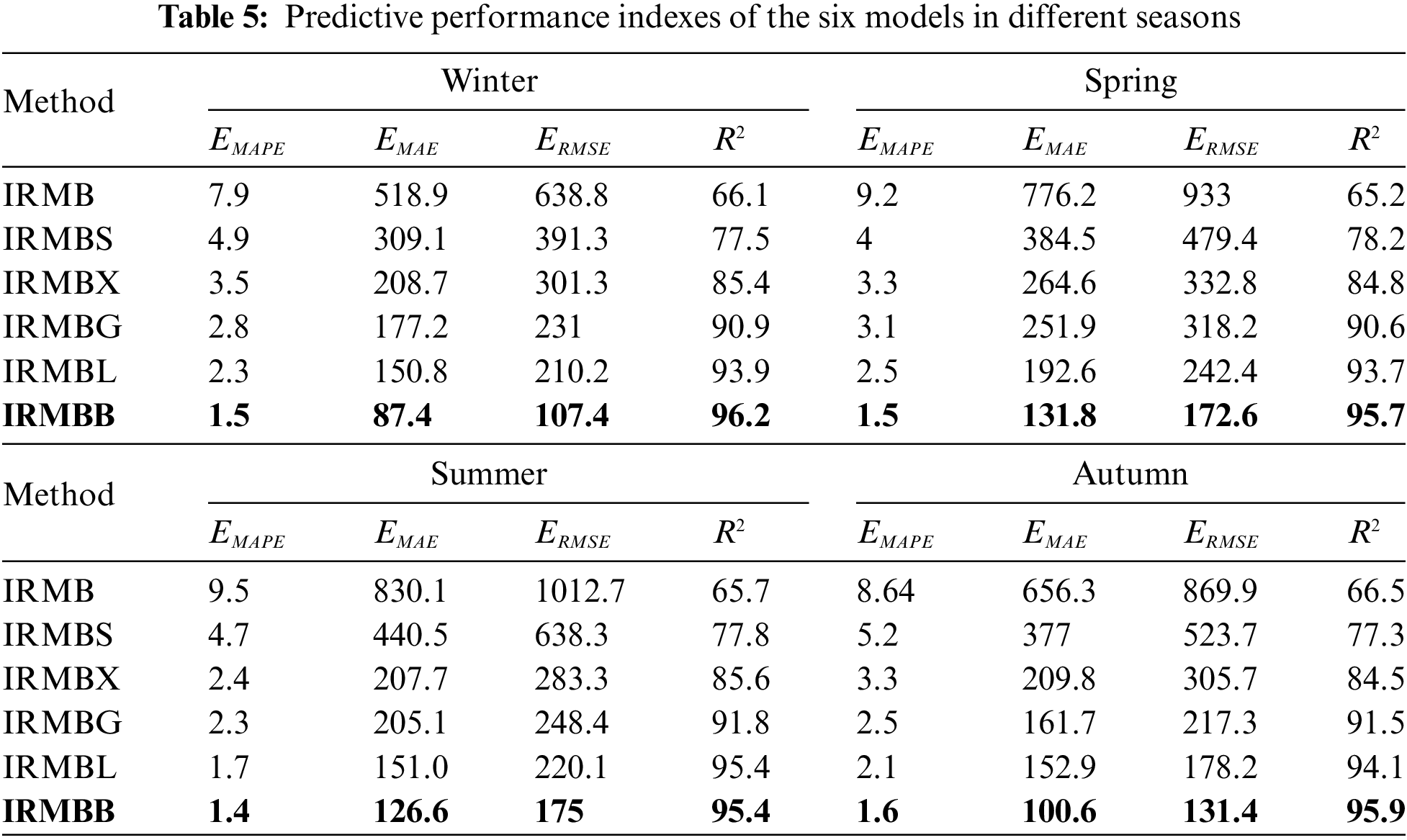
The proposed IRMBB technique outperforms alternative combined models in all four seasons in terms of the evaluation criteria (Table 5). Compared with LSTM and GRU, which are benchmark models in the field of deep learning, BiLSTM exhibits slightly better EMAPE, EMAE, and ERMSE values owing to its capability to capture the bidirectional dependence of time series data. Additionally, the EMAPE values of IRMBB for the four seasons fall between 52% and 83% of those of IRMBL and IRMBG. Overall, LSTM marginally outperforms GRU. The prediction performances of SVM and XGBoost, typical models in the machine learning domain, are consistently inferior to those of LSTM and GRU and notably lower than that of BiLSTM. Even for the summer season, when the prediction performance of IRMBX is best, the EMAPE, EMAE and ERMSE values are 1.69, 1.64, and 1.62 times that of IRMBB, respectively. Moreover, for the four seasons, IRMBS yields EMAPE, EMAE, and ERMSE values that are more than twice those of IRMBB. However, without Bayes optimization for BiLSTM, even if the data have undergone processing through the ICEEMDAN-RCMFE method, better prediction results cannot be achieved. For instance, the metrics for IRMB exceed those of IRMBB by more than a factor of 5, reaching a factor of 7 in winter. According to the R2 evaluation metrics, the proposed IRMBB prediction model demonstrates high R2 values, with R2 improvements ranging from 3% to 46% compared with other models. This significant enhancement suggests that IRMBB fits the data better and provides more accurate prediction results.

Fig. 8 displays the violin error plots for the six methods outlined in that section across the four seasons. The overall error of the IRMB method, without Bayesian hyperparameter search, is the largest, followed by IRMBS and IRMBX. The overall error of IRMBG and IRMBL shows minimal difference, with IRMBL slightly outperforming IRMBG, attributable to the larger training set size used in this paper. However, among the six models, the proposed IRMBB exhibits the smallest overall error variation, demonstrating its superior prediction performance. In conclusion, the presented IRMBB approach outperforms the other five methods.

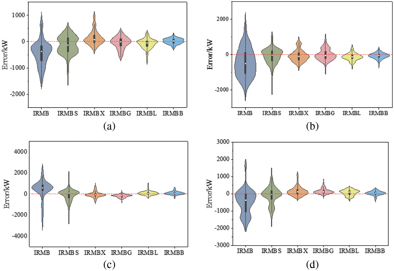
Figure 8: Prediction effects of different models for four seasons: (a) winter; (b) spring; (c) summer; (d) autumn

4.2 Comparative Analysis of Seasonal Short-Term Load Forecasts in Typical Regions

In this paper, a seasonal analysis strategy is adopted for the entire year’s load, wherein the load characteristics of different seasons are considered separately in a more specific manner, and corresponding models are built for different seasonal components. Considering that various seasons exhibit highly varied load fluctuation characteristics, predicting the load separately for different seasons can provide higher-quality input data for the deep-learning-based prediction model. This approach is expected to yield higher load prediction accuracy than methods that do not consider seasonal load variation. The proposed method IRMBB and the five comparison models described in Section 4.1.2 are employed to forecast the extremely-low-temperature weekly load in winter 2020 and the high-temperature weekly load in summer 2021 in Texas, USA, respectively. Two separate training sets are established to form a control: the seasonal training set described in this paper and the traditional continuous training set, which predicts loads using six prediction methods, including IRMBB. Table 6 displays the setup of the training and test sets used for prediction. The raw load statistics for Texas from December 2019 to mid-June 2021 are utilized in this study (Fig. 9). The load forecasting results of the six methods for Texas in 2020 under extremely low temperatures in winter (9 February–15 February, 2021) and 2021 under extremely high temperatures in summer (13 June–19 June, 2021) are evaluated according to the indicators shown in Table 7. The forecast effects are illustrated in Fig. 10.

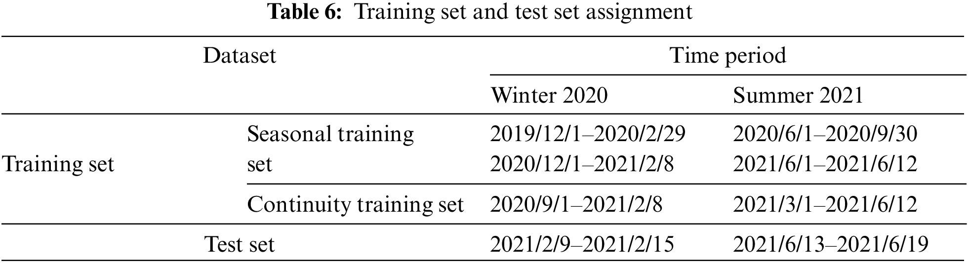
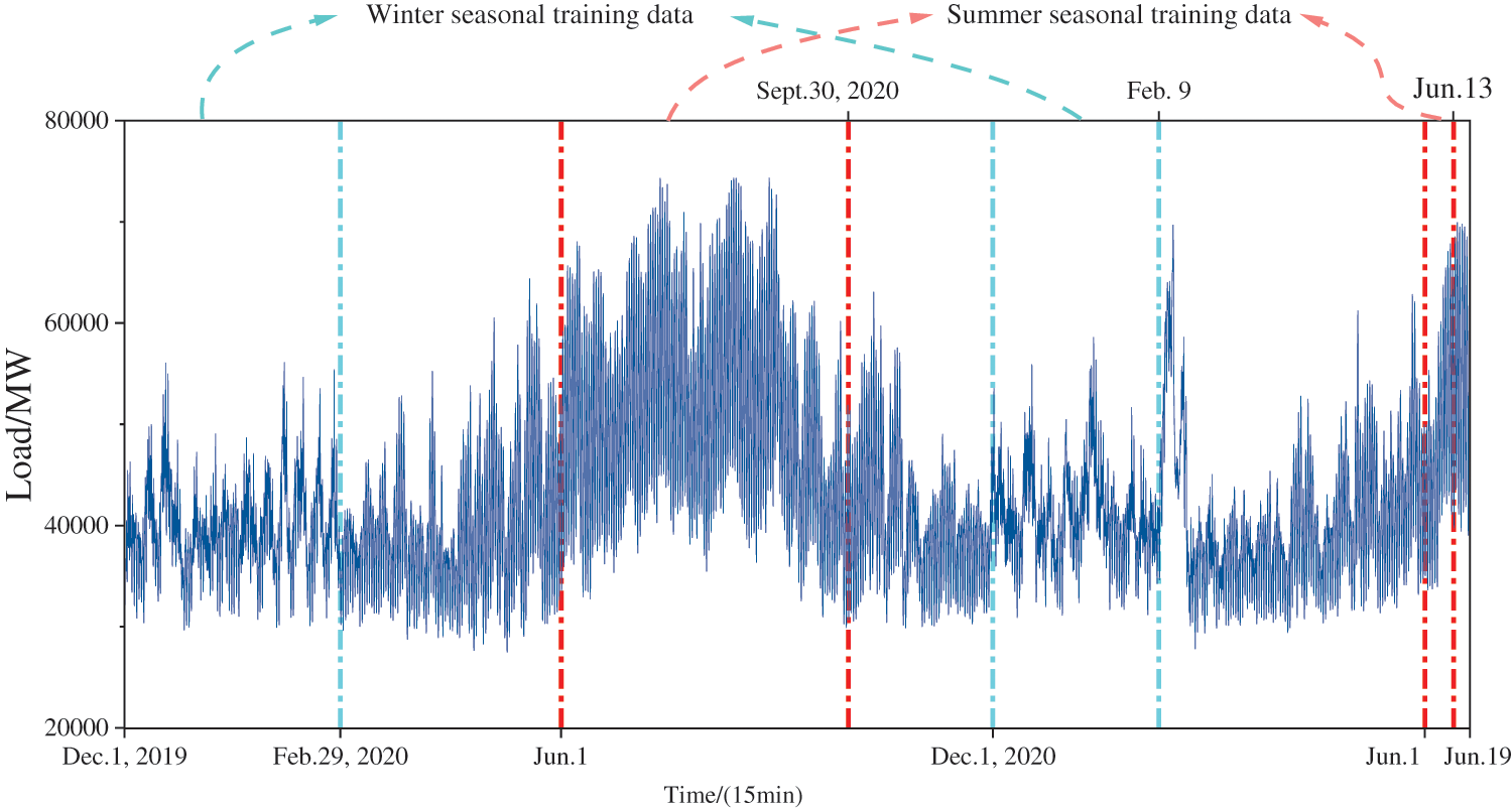
Figure 9: Texas load

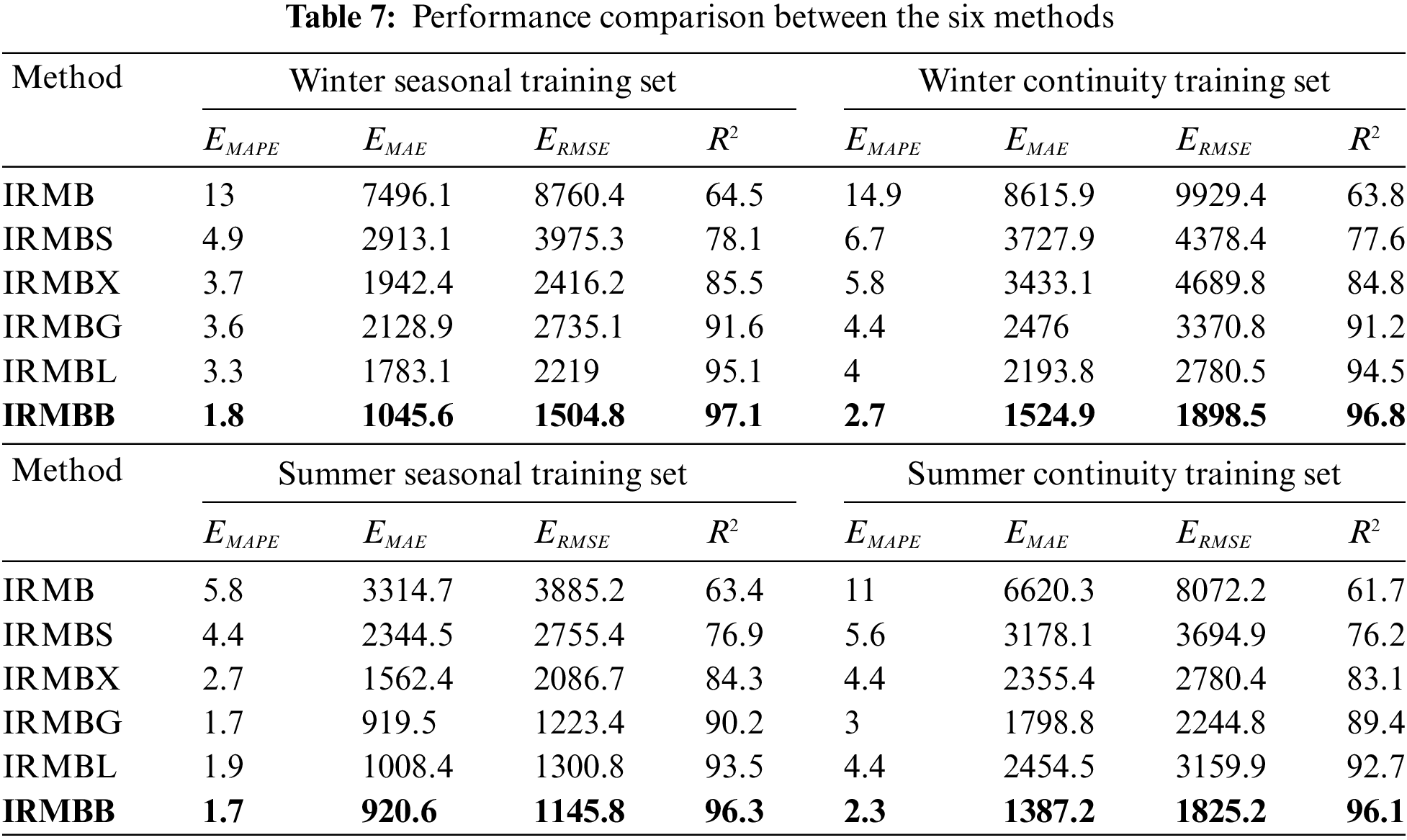
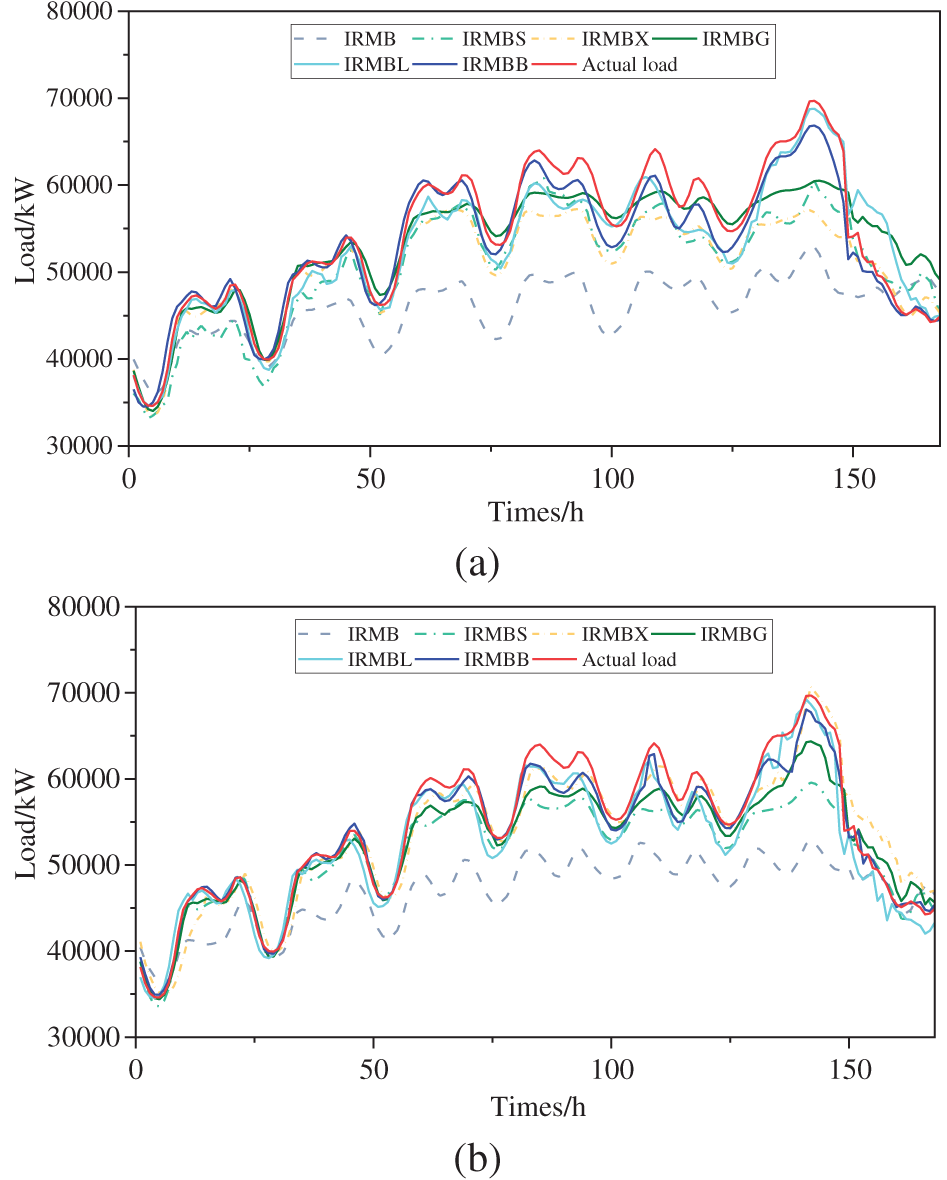
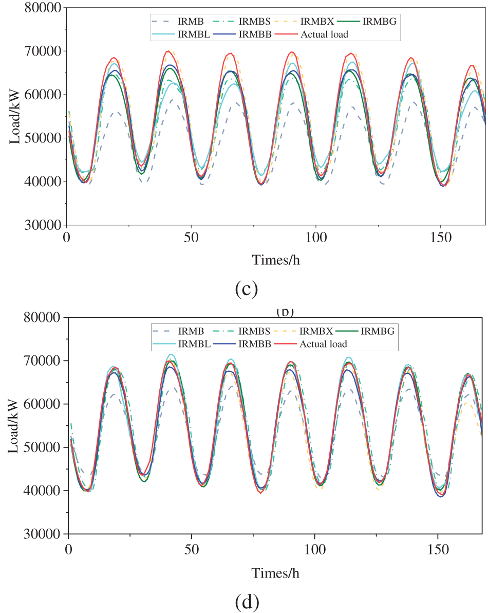
Figure 10: Comparison of prediction results of different models using the seasonal training set and continuous training set under extreme weather conditions (a) winter seasonal training set; (b) winter continuity training set; (c) summer seasonal training set; (d) summer continuity training set

As shown in Table 7, the final predictions of load under extreme weather conditions in Texas obtained through the training of the BiLSTM using the seasonal training set generally outperform those obtained through BiLSTM training using the continuous training set. Owing to the higher volatility and randomness of the load under extreme weather conditions, the EMAPE values of the predicted results of IRMBB obtained using the seasonal training set under extremely low winter temperatures and extremely high summer temperatures are only 1.8% and 1.7%, respectively. These values are only slightly larger than the EMAPE of the predicted load results under normal weather conditions in China, as reported in previous papers. Overall, the proposed IRMBB model outperforms the other five comparison models in predicting load for both winter and summer seasons, with EMAPE values of 2.7% and 2.3%, respectively. This holds even when continuous training data are used, demonstrating the capability of the model to deliver more accurate load predictions.

Additionally, the predictive performance of GRU surpasses that of LSTM when the training dataset size is significantly reduced. For instance, during summer, only 2664 samples are used for training in both sets. Consequently, the EMAPE values for IRMBG in summer are 1.7% and 3%, which are lower than the values for IRMBL (1.9% and 4.4%), and the EMAE and ERMSE values are also smaller than those of IRMBL to some extent. However, when 4032 samples are used for training in winter, the prediction results of IRMBL are superior to those of IRMBG. According to the conclusion that “LSTM is better than GRU,” drawn from a sample set of over 8000 samples across all four seasons, as the training set sample size increases, LSTM and BiLSTM are expected to outperform GRU in predicting load under normal weather conditions in China. This also validates the effectiveness of the proposed ICEEMDAN-RCMFE-mRMR-Bayes-BiLSTM prediction model framework in enhancing load prediction accuracy.

Examination of the prediction effect graphs generated through the six methods using different training sets (Fig. 9) reveals that the proposed IRMBB method aligns better with the actual load profile compared with the other five methods when faced with the sudden increase in grid load during the extreme cold weather in Texas in winter 2020. A comparison of Fig. 9a,b reveals that the load curve generated using the seasonal training set prediction closely resembles the real load curve, particularly for the last day of the weekly load prediction when the load of the Texas grid reaches its peak. Regarding the prediction of the Texas grid load under sweltering weather conditions in June, while the predicted load curve of IRMBB may not perfectly match IRMBX and IRMBL at certain peaks and valleys, the overall contour curve of IRMBB more closely resembles the actual load curve (Fig. 9c,d).

In conclusion, the proposed approach significantly enhances load forecasting accuracy and effectiveness compared with methods that overlook seasonal variation. Compared with previously reported methods, the introduced IRMBB approach, which accounts for seasonal variations, emerges as a more effective multi-feature fusion approach.

5  Conclusion

This paper proposes a seasonal short-term load combination prediction model (IRMBB) for a power system. This model is based on modal decomposition and a feature-fusion multi-algorithm hybrid neural network to address the relatively strong randomness and load fluctuations in four seasons. The working principle and advantages of the model are theoretically analyzed, and the results are consistent with outcomes from actual examples, which validates the efficacy of the suggested approach. The research conducted for this study demonstrates the following:

(1) The proposed IRMBB model enhances prediction accuracy while reducing the number of late prediction tasks through a series of processes, including modal decomposition, complexity evaluation, sequence aggregation, and hyperparameter search on the raw power system load data for each season. Compared with existing combined models, the proposed technique demonstrates superior performance in terms of high prediction accuracy and prediction time, thereby improving the effectiveness of short-term load forecasting for power systems.

(2) Compared with currently used combination models and optimization algorithms (IRMB, IRMBS, IRMBX, IRMBL, and IRMBG), the proposed IRMBB model is more suitable for decomposing loads across the four seasons and extracting essential features. The evaluation index values of the prediction results are overall superior to those of the aforementioned five model groups.

(3) This paper adopts a seasonal analysis strategy for a full year of load. Matching models are created by separately accounting for the varying load characteristics across different seasons. Comparative analyses of actual cases from domestic and international contexts reveal that the proposed method achieves higher load prediction accuracy than methods that do not consider seasonal load variation. This is attributed to the significant differences in load variation characteristics across different seasons, which enable the provision of higher-quality input data for deep-learning-based prediction models.

(4) The proposed model leverages seasonal variation information to enhance the accuracy of short-term load forecasting for power systems. The model is well-suited for applications in power markets and grid management that demand precise forecasting, demonstrating its potential applications for power system operation and planning. However, given that different industries exhibit unique load variation patterns, employing a single short-term power system load forecasting algorithm for all sectors may not fully address the distinct load characteristics of each industry. Therefore, future research should focus on developing tailored short-term load forecasting algorithms for power systems based on the specific needs of each industry, to achieve accurate predictions of load changes in diverse sectors.

Acknowledgement: The Editor-in-Chief, Associate Editor, and anonymous reviewers are gratefully acknowledged by the authors for their assistance with this research.

Funding Statement: The authors received no specific funding for this study.

Author Contributions: Jiachang Liu: Data analysis, Paper writing, Investigation. Zhengwei Huang: Adjusted the overall structure of the paper. Junfeng Xiang: Data curation, Investigation. Lu Liu: Methodology, Article idea, Results analysis. Manlin Hu: Article idea, Visualization. All authors reviewed the results and approved the final version of the manuscript.

Availability of Data and Materials: The original contributions presented in the study are included in the article; further inquiries can be directed to the corresponding author.

Ethics Approval: Not applicable.

Conflicts of Interest: The authors declare that the research was conducted in the absence of any commercial or financial relationships that could be construed as a potential conflict of interest.

References

1. N. Amral, C. S. Ozveren, and D. King, “Short term load forecasting using multiple linear regression,” in 2007 42nd Int. Univ. Power Eng. Conf., Brighton, UK, IEEE, Sep. 2007, pp. 1192–1198. doi: 10.1109/UPEC.2007.4469121. [Google Scholar] [CrossRef]

2. J. P. Hermias, K. Teknomo, and J. C. N. Monje, “Short-term stochastic load forecasting using autoregressive integrated moving average models and hidden markov model,” in 2017 Int. Conf. Inf. Commun. Technol. (ICICT), Karachi, IEEE, Dec. 2017, pp. 131–137. doi: 10.1109/ICICT.2017.8320177. [Google Scholar] [CrossRef]

3. W. Christiaanse, “Short-term load forecasting using general exponential smoothing,” IEEE Trans. Power Apparatus Syst., vol. 90, no. 2, pp. 900–911, Mar. 1971. doi: 10.1109/TPAS.1971.293123. [Google Scholar] [CrossRef]

4. J. Zheng, C. C. Xu, Z. A. Zhang, and X. H. Li, “Electric load forecasting in smart grids using long-short-term-memory based recurrent neural network,” in 2017 51st Annual Conf. Inf. Sci. Syst. (CISS), Baltimore, MD, USA, IEEE, Mar. 2017, pp. 1–6. doi: 10.1109/CISS.2017.7926112. [Google Scholar] [CrossRef]

5. H. Quan, D. Srinivasan, and A. Khosravi, “Short-term load and wind power forecasting using neural network-based prediction intervals,” IEEE Trans. Neural Netw. Learn. Syst., vol. 25, no. 2, pp. 303–315, Feb. 2014. doi: 10.1109/TNNLS.2013.2276053. [Google Scholar] [PubMed] [CrossRef]

6. C. N. Ko and C. M. Lee, “Short-term load forecasting using SVR (support vector regression)-based radial basis function neural network with dual extended Kalman filter,” Energy, vol. 49, no. 12, pp. 413–422, Jan. 2013. doi: 10.1016/j.energy.2012.11.015. [Google Scholar] [CrossRef]

7. G. F. Fan, L. L. Peng, W. C. Hong, and F. Sun, “Electric load forecasting by the SVR model with differential empirical mode decomposition and auto regression,” Neurocomputing, vol. 173, pp. 958–970, Jan. 2016. doi: 10.1016/j.neucom.2015.08.051. [Google Scholar] [CrossRef]

8. B. Li and M. Z. Lu, “Short-term load forecasting modeling of regional power grid considering real-time meteorological coupling effect,” (in Chinese), AEPS, vol. 44, no. 17, pp. 60–68, Sep. 2020. [Google Scholar]

9. H. Shi, M. H. Xu, and R. Li, “Deep learning for household load forecasting—a novel pooling deep RNN,” IEEE Trans. Smart Grid, vol. 9, no. 5, pp. 5271–5280, Sep. 2018. doi: 10.1109/TSG.2017.2686012. [Google Scholar] [CrossRef]

10. A. Haque and S. Rahman, “Short-term electrical load forecasting through heuristic configuration of regularized deep neural network,” Appl. Soft Comput., vol. 122, no. 12, pp. 108877, Jun. 2022. doi: 10.1016/j.asoc.2022.108877. [Google Scholar] [CrossRef]

11. J. Gunawan and C. Y. Huang, “An extensible framework for short-term holiday load forecasting combining dynamic time warping and LSTM network,” IEEE Access, vol. 9, pp. 106885–106894, 2021. doi: 10.1109/ACCESS.2021.3099981. [Google Scholar] [CrossRef]

12. K. Ijaz, Z. Hussain, J. Ahmad, S. F. Ali, M. Adnan, and I. Khosa, “A novel temporal feature selection based LSTM model for electrical short-term load forecasting,” IEEE Access, vol. 10, pp. 82596–82613, 2022. doi: 10.1109/ACCESS.2022.3196476. [Google Scholar] [CrossRef]

13. Y. X. Guo et al., “BiLSTM multitask learning-based combined load forecasting considering the loads coupling relationship for multienergy system,” IEEE Trans. Smart Grid, vol. 13, no. 5, pp. 3481–3492, Sep. 2022. doi: 10.1109/TSG.2022.3173964. [Google Scholar] [CrossRef]

14. S. B. Hu et al., “Short-term load forecasting based on mutual information and BI-LSTM considering fluctuation in importance values of features,” IEEE Access, vol. 12, pp. 23653–23665, 2024. doi: 10.1109/ACCESS.2023.3323403. [Google Scholar] [CrossRef]

15. M. J. Chen, F. H. Qiu, X. Z. Xiong, Z. W. Chang, Y. Wei and J. Wu, “BILSTM-SimAM: An improved algorithm for short-term electric load forecasting based on multi-feature,” MBE, vol. 21, no. 2, pp. 2323–2343, 2024. doi: 10.3934/mbe.2024102. [Google Scholar] [PubMed] [CrossRef]

16. N. Kim, H. Park, J. Lee, and J. K. Choi, “Short-term electrical load forecasting with multidimensional feature extraction,” IEEE Trans. Smart Grid, vol. 13, no. 4, pp. 2999–3013, Jul. 2022. doi: 10.1109/TSG.2022.3158387. [Google Scholar] [CrossRef]

17. B. B. Yu, J. J. Li, C. Liu, and B. Sun, “A novel short-term electrical load forecasting framework with intelligent feature engineering,” Appl. Energy, vol. 327, no. 11, pp. 120089, Dec. 2022. doi: 10.1016/j.apenergy.2022.120089. [Google Scholar] [CrossRef]

18. H. T. Zheng, J. B. Yuan, and L. Chen, “Short-term load forecasting using EMD-LSTM neural networks with a Xgboost algorithm for feature importance evaluation,” Energies, vol. 10, no. 8, pp. 1168, Aug. 2017. doi: 10.3390/en10081168. [Google Scholar] [CrossRef]

19. H. Liu, H. Q. Tian, X. F. Liang, and Y. Li, “Wind speed forecasting approach using secondary decomposition algorithm and Elman neural networks,” Appl. Energy, vol. 157, no. 8, pp. 183–194, Nov. 2015. doi: 10.1016/j.apenergy.2015.08.014. [Google Scholar] [CrossRef]

20. G. F. Fan, Y. R. Liu, H. Z. Wei, M. Yu, and Y. H. Li, “The new hybrid approaches to forecasting short-term electricity load,” Elect. Power Syst. Res., vol. 213, no. 2, pp. 108759, Dec. 2022. doi: 10.1016/j.epsr.2022.108759. [Google Scholar] [CrossRef]

21. W. J. Zhang and W. Huang, “Multivariate load prediction method for integrated energy system based on CEEMD-LSTM,” IOP Conf. Ser.: Earth Environ. Sci., vol. 772, no. 1, pp. 012055, May 2021. doi: 10.1088/1755-1315/772/1/012055. [Google Scholar] [CrossRef]

22. K. Li, W. Huang, G. Y. Hu, and J. Li, “Ultra-short term power load forecasting based on CEEMDAN-SE and LSTM neural network,” Energy Build., vol. 279, no. 84, pp. 112666, Jan. 2023. doi: 10.1016/j.enbuild.2022.112666. [Google Scholar] [CrossRef]

23. Y. Ren, P. N. Suganthan, and N. Srikanth, “A comparative study of empirical mode decomposition-based short-term wind speed forecasting methods,” IEEE Trans. Sustain. Energy, vol. 6, no. 1, pp. 236–244, Jan. 2015. doi: 10.1109/TSTE.2014.2365580. [Google Scholar] [CrossRef]

24. H. C. Peng, F. H. Long, and C. Ding, “Feature selection based on mutual information criteria of max-dependency, max-relevance, and min-redundancy,” IEEE Trans. Pattern Anal. Mach. Intell., vol. 27, no. 8, pp. 1226–1238, Aug. 2005. doi: 10.1109/TPAMI.2005.159. [Google Scholar] [PubMed] [CrossRef]

25. Y. X. Zhao, X. Wang, C. W. Jiang, J. H. Zhang, and Z. Q. Zhou, “A novel short-term electricity price forecasting method based on correlation analysis with the maximal information coefficient and modified multi-hierachy gated LSTM,” (in Chinese), Proc. CSEE, vol. 41, no. 1, pp. 135–146, Jan. 2021. [Google Scholar]

26. J. Wu, F. Miu, and T. Y. Li, “Daily crude oil price forecasting based on improved CEEMDAN, SCA, and RVFL: A case study in WTI oil market,” Energies, vol. 13, no. 7, pp. 1852, Apr. 2020. doi: 10.3390/en13071852. [Google Scholar] [CrossRef]

27. S. Z. Gao, Q. Wang, and Y. M. Zhang, “Rolling bearing fault diagnosis based on CEEMDAN and refined composite multiscale fuzzy entropy,” IEEE Trans. Instrum. Meas., vol. 70, pp. 1–8, 2021. doi: 10.1109/TIM.2021.3072138. [Google Scholar] [CrossRef]

28. J. D. Zheng, H. Y. Pan, J. Y. Tong, and Q. Y. Liu, “Generalized refined composite multiscale fuzzy entropy and multi-cluster feature selection based intelligent fault diagnosis of rolling bearing,” ISA Trans., vol. 123, no. 5, pp. 136–151, Apr. 2022. doi: 10.1016/j.isatra.2021.05.042. [Google Scholar] [PubMed] [CrossRef]

29. M. Schuster and K. K. Paliwal, “Bidirectional recurrent neural networks,” IEEE Trans. Signal Process., vol. 45, no. 11, pp. 2673–2681, Nov. 1997. doi: 10.1109/78.650093. [Google Scholar] [CrossRef]

30. X. J. Gong, R. J. Zhu, and B. Tang, “Short-term peak load prediction based on bayesian optimisation XGBoost,” (in Chinese), Electric Power Eng. Technol., vol. 39, no. 6, pp. 76–81, Nov. 2020. [Google Scholar]

31. W. Hu, X. Y. Zhang, Z. E. Li, Q. Li, and H. Wang, “Short-term load forecasting based on an optimized VMD-mRMR-LSTM model,” (in Chinese), Power Syst. Prot. Control, vol. 50, no. 1, pp. 88–97, Jan. 2022. [Google Scholar]

32. B. Q. Bai, J. T. Liu, X. Wang, C. W. Jiang, T. Jiang and S. X. Zhang, “Short-term multivariate load forecasting for urban energy based on minimum redundancy maximum relevance and dual-attention mechanism,” (in Chinese), Power Syst. Autom., vol. 46, no. 17, pp. 44–55, Sep. 2022. [Google Scholar]

33. R. L. Hu, Y. C. Chen, D. H. Zhang, P. Zhang, S. Y. Wang and Y. Yu, “Bus load prediction method based on SSA-Bi-LSTM neural network,” (in Chinese), Guangdong Electric Power, vol. 35, no. 2, pp. 19–26, Feb. 2022. [Google Scholar]

34. J. C. Guo et al., “Multi-objective optimization design and multi-attribute decision-making method of a distributed energy system based on nearly zero-energy community load forecasting,” Energy, vol. 239, no. 3, pp. 122124, Jan. 2022. doi: 10.1016/j.energy.2021.122124. [Google Scholar] [CrossRef]

35. Q. Li, J. Li, and H. Ma, “Short-term electric load forecasting based on complementary integrated empirical modal decomposition-fuzzy entropy and echo state network,” (in Chinese), Comput. Appl., vol. 34, no. 12, pp. 3651–3655+3659, Dec. 2014. [Google Scholar]

36. X. M. Yang, X. Cui, B. Zhou, and Z. Peng, “Short-term load forecasting based on particle swarm optimisation support vector machine,” J. Wuhan Univ. (Eng. Ed.), vol. 51, no. 8, pp. 715–720, Aug. 2018. [Google Scholar]

37. Z. Y. Chen et al., “Ultra-short-term power load forecasting based on combined LSTM and XGBoost models,” Power Grid Technol., vol. 44, no. 2, pp. 614–620, Feb. 2020 (In Chinese). [Google Scholar]

38. Z. Zou, T. Z. Wu, X. X. Zhang, and Z. M. Zhang, “Short-term load forecasting based on Bayesian optimised CNN-BiGRU hybrid neural network,” (in Chinese), High Volt. Technol., vol. 48, no. 10, pp. 3935–3945, Oct. 2022. [Google Scholar]