SOH Estimation of Lithium Batteries Based on ICA and WOA-RBF Algorithm

Nomenclature

1  Introduction

With the increasingly serious energy crisis and environmental issues [1], electric vehicles have developed rapidly, and their safe operation has received increasing attention. Lithium ion batteries have high energy and power densities [2], and their health status is an important factor for the stable operation of electric vehicles. SOH, also known as battery health status, is commonly used to describe the degree of battery aging. As the number of cycles of the battery increases, the degree of battery aging also intensifies, and the SOH value of the battery decreases, which may become difficult to meet the application requirements of on-board electrical equipment. Therefore, accurate estimation of battery SOH plays an important role in estimating the State of Charge (SOC) and balancing the battery.

Battery SOH is a measure that reflects the current state of a battery, including its capacity and power output capability, as well as its ratio to its initial state, and its use is monitored using battery management systems (BMSs) [3]. There are currently two commonly used standards for defining battery SOH, one is based on the remaining capacity of the battery, and the other is based on the internal resistance of the battery. This article uses the definition of remaining battery capacity because capacity is easier to measure compared to internal resistance. The SOH defined based on remaining capacity is as follows: SOH=Cap(i)Cap(0)×100%, where Cap(i) represents the i remaining capacity of the second cycle and Cap(0) represents the rated capacity. The estimation of battery SOH can be divided into two categories. One is based on battery model methods, which require calibration of battery model parameters to achieve battery SOH estimation, usually combined with SOC estimation. The other is experimental analysis methods, which convert the collected voltage and current parameters into features that can indicate battery performance degradation and use these features to estimate battery SOH.

A large number of scholars have proposed specific estimation methods for the aforementioned SOH estimation methods. Reference [4] proposed a battery SOH estimation method using a dual adaptive extended particle filter. This method utilizes extended Kalman to linearize the particle distribution function, reducing the impact of model parameter changes on estimating battery SOH. However, this experiment only achieved good estimation results near local SOH values, and it cannot be seen that the overall SOH decline process can still achieve good estimation results; Reference [5] proposed a multi time scale model (dual Kalman) parameter identification method for the slow changing characteristics of battery parameters and the fast changing characteristics of states, which effectively improves the robustness of battery SOH estimation by estimating battery SOC and inferring battery SOH. However, when using Kalman to estimate battery SOC, the value of SOH needs to be known, so this method requires periodic calibration of SOH values to obtain accurate SOC values and estimate battery SOH in real time; Reference [6] proposed a lithium battery SOH estimation method based on the SR-UKF algorithm. By establishing an equivalent circuit model and estimating the internal resistance of the battery in real time, the battery SOH was estimated. However, only a relatively simple operating condition was selected for verification, which is not universal; Reference [7] designed a data preprocessing method for the optimal variational mode, introduced a weighted vector method, and fused it with support vector machines to establish a new estimation model, effectively solving the problem of inaccurate battery SOH estimation caused by capacity regeneration. However, after the optimal variational mode decomposition, the data changed from one group to three groups, requiring simultaneous training of these three types of data and increasing computational complexity; Reference [8] developed an online estimation model that can simultaneously estimate SOC and SOH in real-time, using discharge voltage and ground voltage drop per unit time as model parameters, achieving stability in battery parameter estimation. However, in terms of SOH accuracy testing, only fixed points are tested, and the accuracy at other points is unknown. Reference [9] designed a stacked LSTM neural network to train and test the constant current measurement values during fast charging, which has good estimation performance for SOH estimation in fast charging. However, stacking multiple LSTM neural networks makes the network structure complex.

The difference and similarity between this method and the above methods are that (1) traditional equivalent circuits are not used as the model for battery SOH estimation, which is greatly affected by battery SOC. Instead, machine learning model method based on ICA curve method is adopted, which is supported by a large amount of charge and discharge data and does not need to consider the influence of battery SOC; (2) In the same estimation strategy based on machine learning, this article proposes the WOA-RBF algorithm. Compared with other machine learning algorithms, the RBF algorithm has the advantages of a simple network structure and better local response. In addition, the WOA algorithm has strong global search ability and fast convergence speed, which can accurately and quickly find the optimal parameters of the RBF model, achieving the accurate estimation of battery SOH by the WOA-RBF algorithm.

2  Data Preprocessing

2.1 Dataset Introduction

The dataset used in this article is a prismatic battery with a nominal capacity of 1100 mAh, designated as CS2-36, publicly available at the University of Maryland. Due to the fact that a small rate of charging and discharging current can better extract features that characterize the changes in battery SOH, and batteries with a capacity lower than 80% of the initial capacity are considered failed batteries. Therefore, a small magnification charging dataset with a remaining capacity of 100%–80% of the initial capacity was selected. Battery was tested using the Arbin Battery Tester. The specific operation process is as follows. (1) Charge the battery to 4.2 V using a constant current charging method of 0.5 C, (2) Charge the battery current to below 0.05 A using a constant voltage charging method of 4.2 V, (3) Discharge at a rate of 1 C to the battery cut-off voltage of 2.7 V, (4) Cycle steps (1), (2) and (3) until the battery capacity drops to around 80%. Fig. 1 shows the remaining capacity variation curve of the battery after 463 cycles.

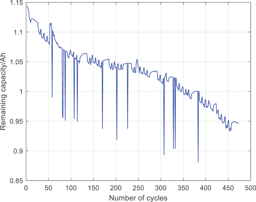
Figure 1: The variation of battery capacity with the number of battery discharge cycles

2.2 Abnormal Data Elimination

From the capacity change chart, it can be seen that after many cycles, the capacity increases compared to the previous one, which is a phenomenon of capacity increase. That is, if the battery is left idle for a period of time after several cycles, the next discharge capacity will increase, which is a normal phenomenon. Some cycles show a significant drop in capacity after completion, and the capacity returns to normal values in the next cycle, which is obviously abnormal. The solution is to set a capacity decrease threshold. If it exceeds this threshold, it is considered abnormal data and needs to be removed. Fig. 2 shows the capacity decline curve after removing abnormal data. To obtain the capacity change curve, it is necessary to convert it into battery SOH. Take the discharge capacity of the first cycle as the initial capacity, and calculate the ratio of each discharge capacity to the initial battery capacity to obtain the battery SOH for the current cycle. Fig. 3 shows the variation curve of battery SOH with the number of battery discharge cycles.

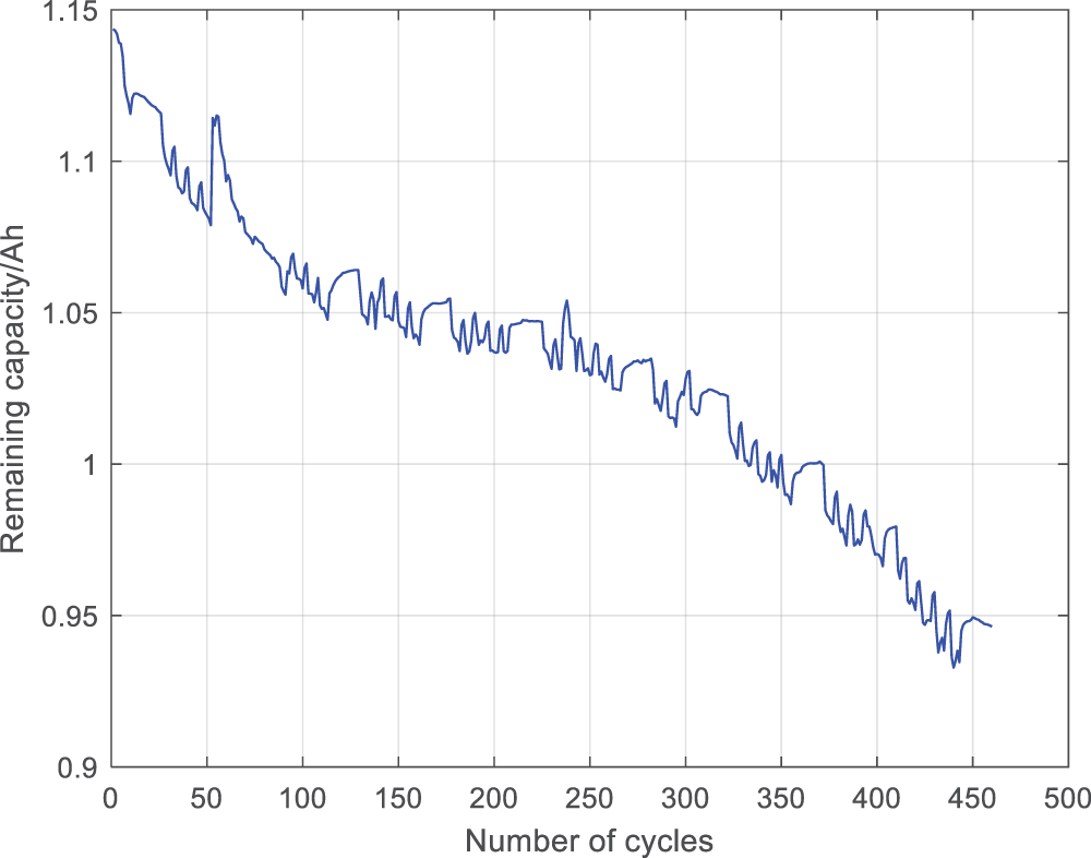
Figure 2: Changes in battery capacity with number of discharge cycles after removing abnormal data

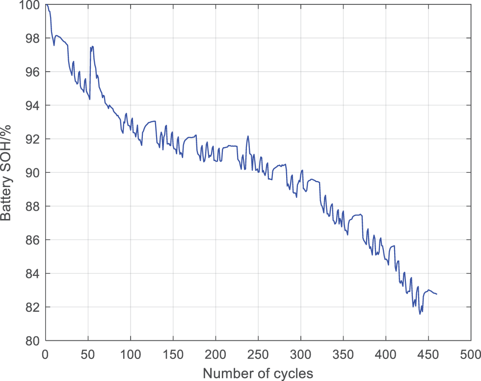
Figure 3: The variation curve of battery SOH with the number of battery discharge cycles

3  IC Curve Acquisition

This article uses ICA as the method for feature extraction because it is a non-destructive tool that can explain the subtle changes during the aging process of power batteries. Capacity increment refers to the capacity of a battery to charge and discharge within a unit voltage range at a certain current [10]. Compared to the original curve, the most obvious feature of the IC curve is the IC peak, and each IC peak represents the electrochemical process that occurs inside the power battery, with a unique shape, height, and position. Therefore, any change in the position and shape of the IC peak is a manifestation of the aging of the power battery.

3.1 Q-V Curve for Constant Current Charging

Before obtaining the IC curve, it is necessary to obtain the Q-V curve of constant current charging, that is, during the offline training stage, extract the charging process from the battery degradation dataset and analyze the features of battery capacity degradation [11]. Fig. 4 shows the relationship between capacity and voltage changes during a certain cycle. It can be seen from the graph that the Q-V curve does not increase linearly. In the initial stage of charging, the voltage rises rapidly. As the charging current flows in, the voltage and capacity also increase rapidly, but the rate of increase is different and constantly changing. Therefore, it is necessary to convert this subtle rate change into intuitive rate data.

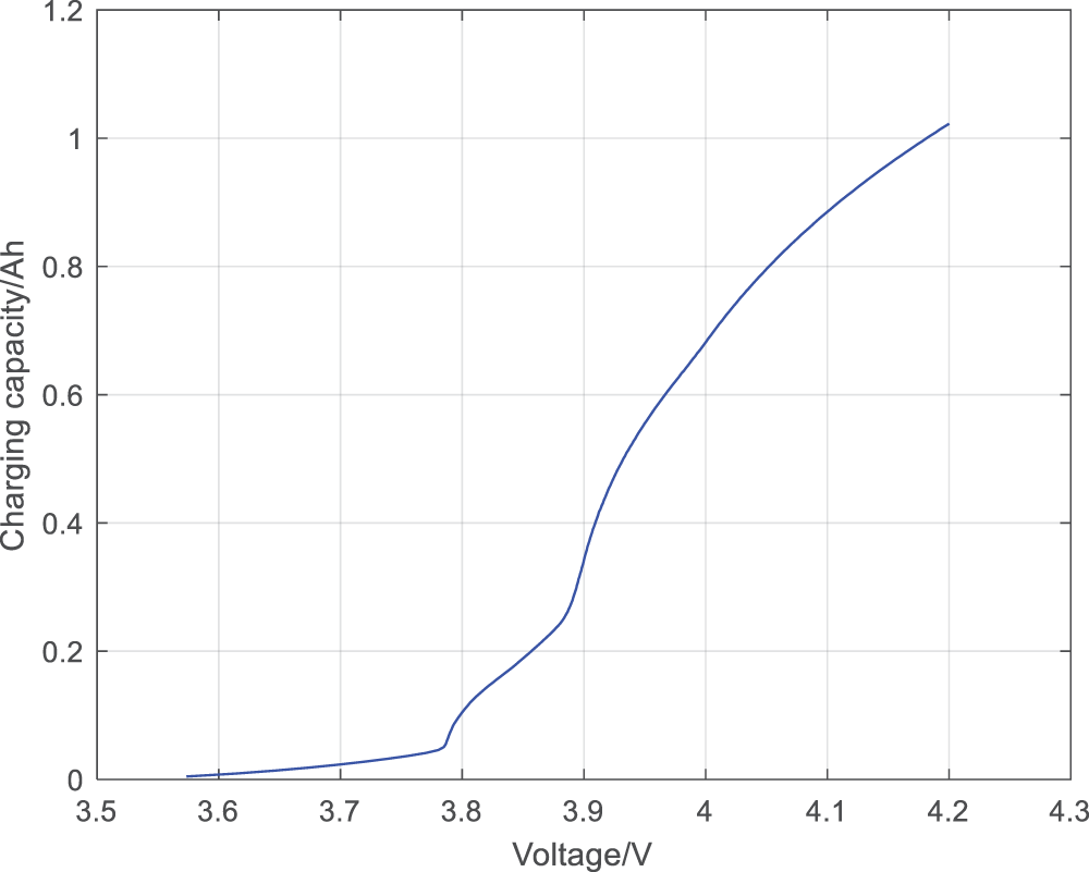
Figure 4: Relationship between voltage and capacity changes during a single charging process

3.2 IC Curve

The ICA curve method organizes the initial charging data to obtain the dQ/dV data during the charging or discharging process, and then obtains the capacity change rate-terminal voltage (dQ/dV‐V) curve, as shown in the figure. The principle of IC curve is to calculate the first derivative of the Q-V curve of the battery under constant current charging or discharging conditions to obtain the dQ/dV‐Vcurve. To solve the first-order derivative of the IC curve, it is necessary to first perform function fitting on the Q‐V curve, which inevitably introduces fitting errors. Therefore, this article adopts a simple and practical method to draw the IC curve, ΔV replacing it with a fixed voltage interval ΔQ to represent the ΔV capacity change in the corresponding interval. When it ΔV approaches 0, it is approximately dQdV≈ΔQΔV. Fig. 5 shows the IC curve derived from the Q-V curve variation.

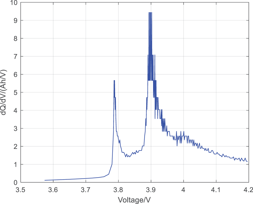
Figure 5: IC curve

3.3 Wavelet Threshold Denoising

Wavelet transform can perform finer processing on signals and better express certain features of the signal [12]. From the perspective of the capacity increment curve, the curve has high noise and is not smooth enough, which is not conducive to collecting the required sample points. Therefore, it is necessary to denoise the IC curve. There are many methods that can be used to handle the noise of capacity increment curves, such as sliding average filtering, first-order low-pass filtering, wavelet packet transform, Fourier transform, etc. In this article, considering the simplicity of operation and good filtering effect, wavelet threshold filtering is chosen. By selecting appropriate decomposition levels, threshold rules, and processing methods, noise in the signal can be effectively removed while retaining useful information, achieving wavelet denoising function. The specific parameter settings are as follows: the threshold rule is heursure, the denoising method is soft thresholding, the reconstruction mode is one stage reconstruction, the decomposition level is 5, and the wavelet type is db4. Fig. 6 shows the noise reduction results of the IC curve.

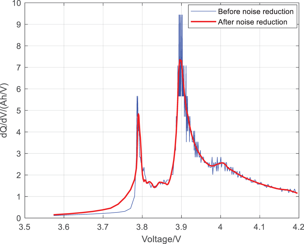
Figure 6: IC curve after noise reduction

4  Feature Parameters and Correlation Analysis of the Health Status of Batteries

4.1 Extraction of Charging Time Features

The charging process of lithium batteries consists of a constant current section (CC) and a constant voltage section (CV). The battery is first charged at a constant current to the charging cut-off voltage, and then charged at a constant cut-off voltage to the cut-off current. The time required to complete the constant current and constant voltage sections varies in different battery health states. However, due to the large proportion of time spent in the constant current section of a typical battery to the entire charging time, the constant current section charging time is chosen as a parameter for battery SOH estimation. In the MATLAB environment, record the charging time t1 at the starting point of the constant current section, and then record the charging time t2 at the ending point of the constant current section. t2−t1 is the charging time of the constant current section. Fig. 7 shows the charging curve of the constant current section as a function of the battery discharge cycle. Fig. 8 shows the relationship between the extracted charging time and the number of battery cycles. Take the battery charging time as the battery health feature 1, denoted as H1.

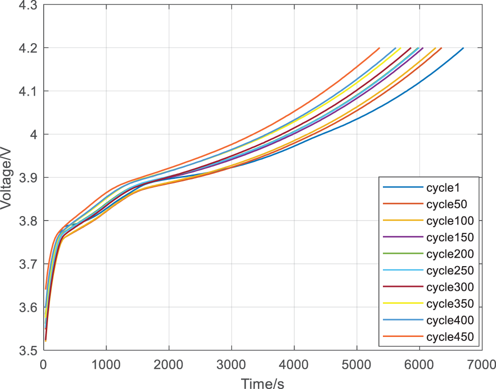
Figure 7: Constant current charging curves under different cycle times

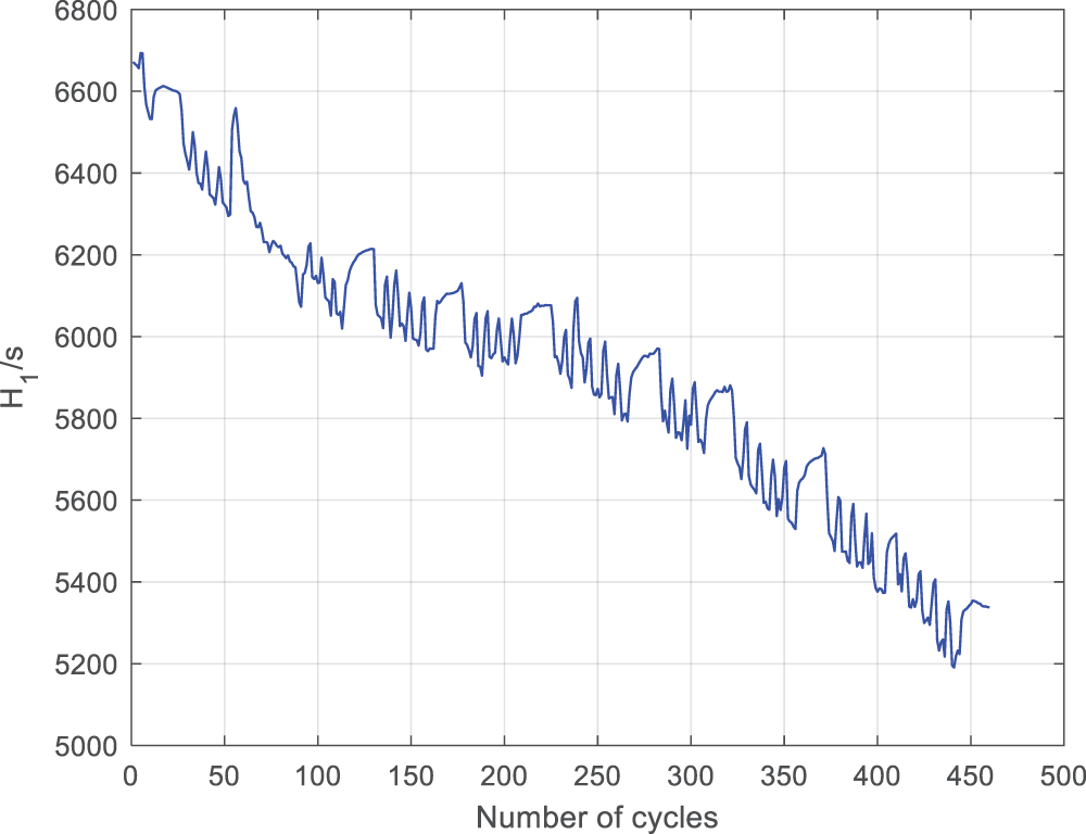
Figure 8: Relationship between H1 and the number of cycles

4.2 Feature Extraction of Capacity Increment Curve

With the intensification of battery aging, the charging and discharging performance of batteries is also deteriorating. In order to accurately reflect the degree of battery aging and estimate the battery SOH, it is necessary to select accurate battery health features. To draw an IC curve, it is necessary to convert it. In this article, an IC curve is drawn every 50 charge and discharge cycles until the battery SOH value is discharged to around 80%, in order to identify the health features that can describe battery aging, as shown in Fig. 9. From the graph, it can be seen that as the number of battery cycles increases, the overall IC curve moves towards the lower right corner of the coordinate axis, with the two IC peaks particularly prominent moving towards the lower right corner of the coordinate axis. Therefore, this article selects the horizontal axis (H2) of the first IC peak, the vertical axis (H3) of the first IC peak, the horizontal axis (H4) of the second IC peak, and the vertical axis (H5) of the second IC peak as the second, third, fourth, and fifth health features of the battery, respectively.

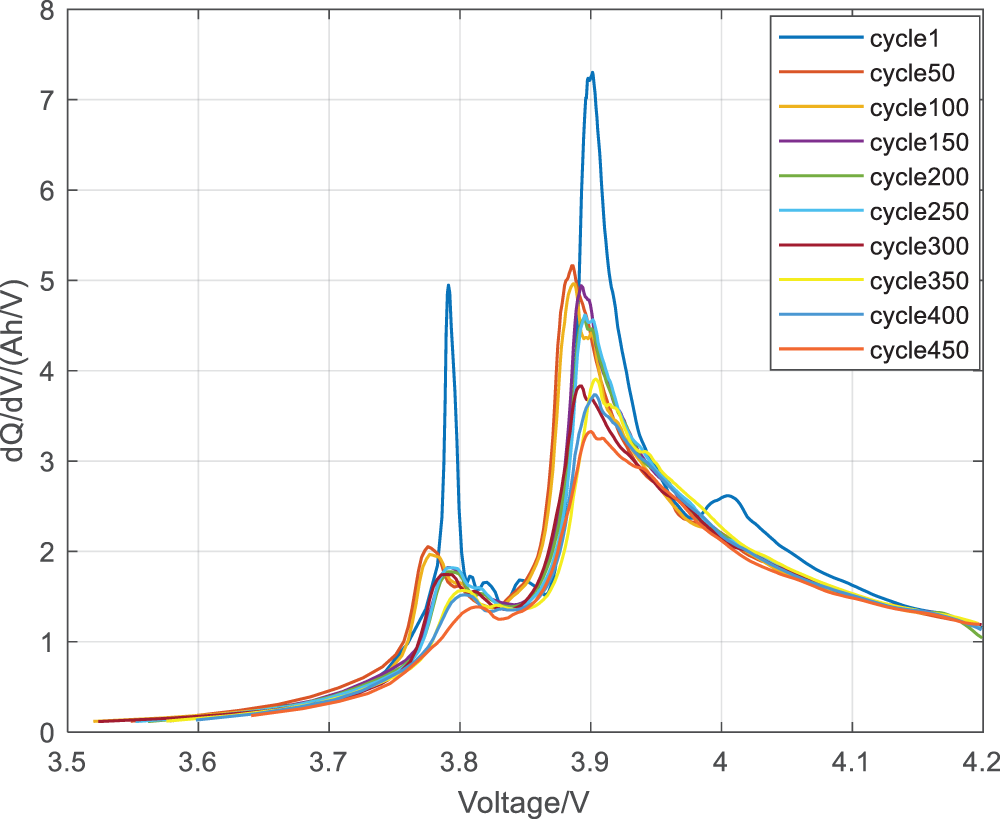
Figure 9: IC curves under different cycles

In the MATLAB environment, extract the horizontal and vertical coordinates of the two peaks of each IC curve as health factors. The specific operation is to divide the IC curve into two parts, left and right, with 3.86 V as the boundary, and determine the peak value of each part in bubble sorting. The variation pattern of the four health features with the number of battery cycles is shown in Figs. 10–13. From the four graphs, it can be seen that the health features H2, H3, and H5 show a significant upward/downward trend with the number of cycles, while the fluctuation of H4 is significant. Therefore, quantitative analysis of health features is necessary.

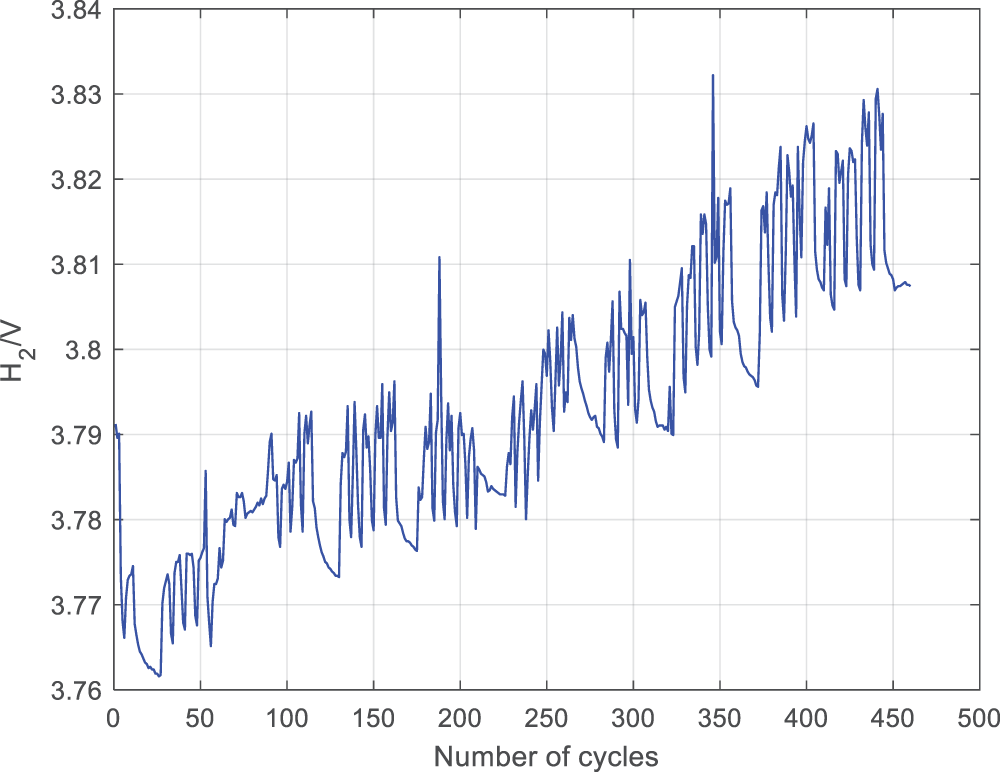
Figure 10: Relationship between H2 and the number of cycles

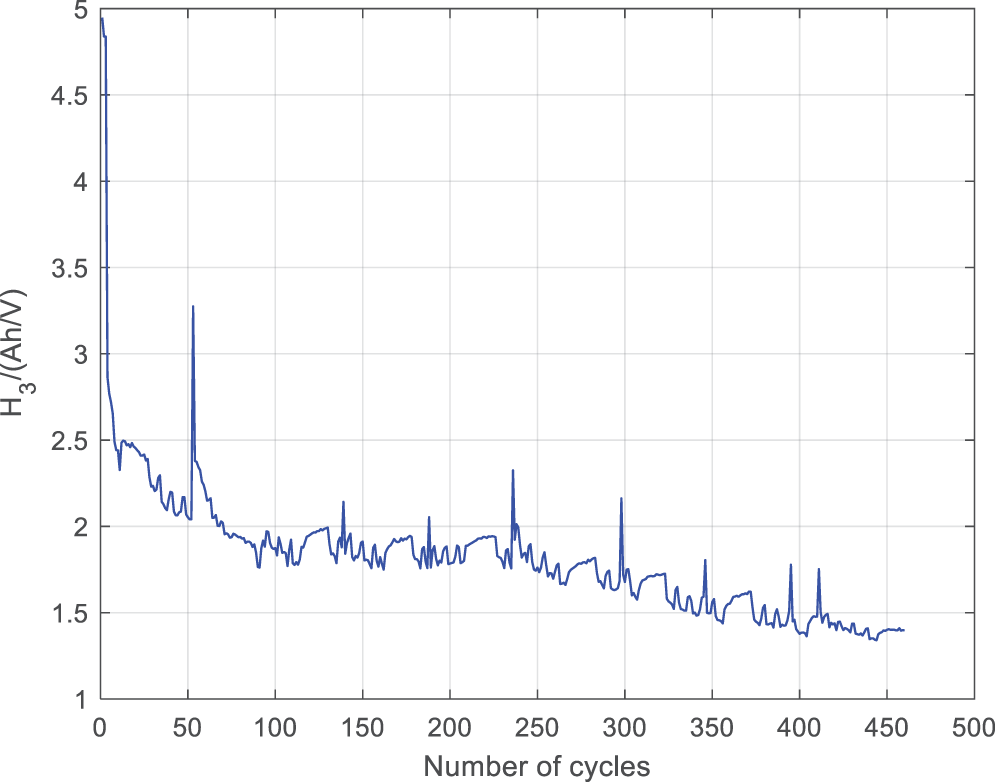
Figure 11: Relationship between H3 and the number of cycles

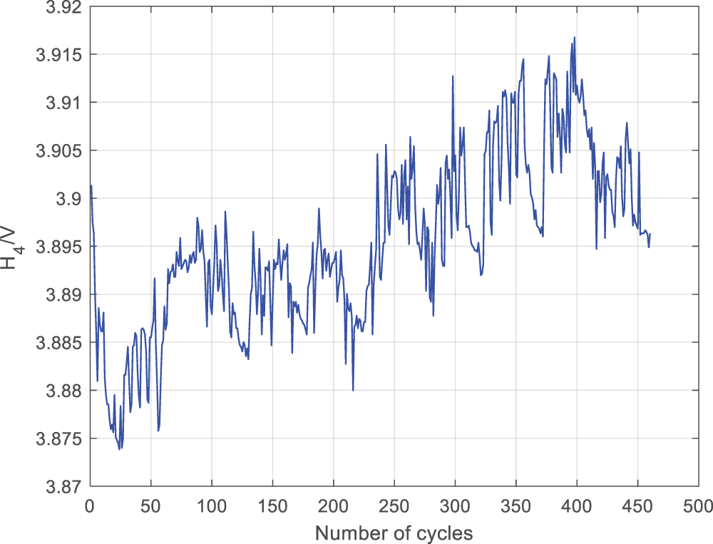
Figure 12: Relationship between H4 and the number of cycles

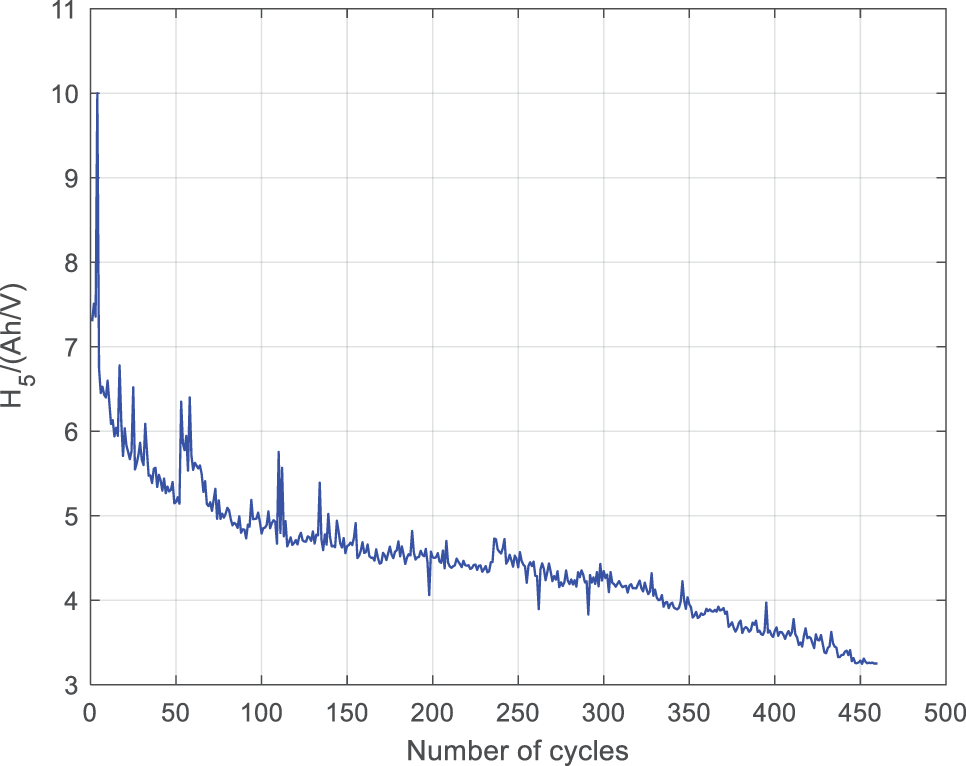
Figure 13: Relationship between H5 and the number of cycles

4.3 Correlation Analysis between Health Features and SOH

In order to quantitatively analyze the relationship between five health features and battery SOH, this article uses the Pearson correlation coefficient method for correlation analysis. The principle is the ratio of the covariance of variables X and Y to the standard deviation of X and Y. The formula is: r=∑i=1N(Xi−X¯)(Yi−Y¯)∑i=1N(Xi−X¯)2∑i=1N(Yi−Y¯)2, where N represents the number of samples, Xi represents the inth observation value of the variable X, X¯ represents the average value of the variable X, Yi represents the inth observation value of the variable Y, and Y¯ represents the average value of the variable Y.

The range of Pearson correlation coefficient is between [−1, 1]. The correlation coefficient shows directionality: if the correlation coefficient is close to 1, it indicates a high positive correlation between the two variables; If the correlation coefficient is close to −1, it indicates a high negative correlation between the two variables; If the correlation coefficient is close to 0, it indicates that the two variables are independent of each other and have no correlation. Specifically, if the absolute value of the Pearson coefficient is between 0.8–1.0, it indicates extreme correlation between the two variables. If it is between 0.6–0.8, it indicates strong correlation between the two variables. If it is between 0.4–0.6, it indicates moderate correlation. If it is between 0.2–0.4, it indicates weak correlation between the two variables. If it is between 0–0.2, it indicates extremely weak or no correlation between the two variables. From the table below, it can be seen that features 1, 2, 3, and 5 have a strong correlation with battery SOH, while feature 4 has a strong correlation with battery SOH. Therefore, all five health features can be used as indicators for battery SOH estimation. Table 1 shows the Pearson coefficients between health factors and battery capacity.

5  WOA-RBF Algorithm for Estimating Battery SOH

5.1 Whale Algorithm WOA

WOA is an algorithm that simulates whales hunting prey, covering three types of predation processes: encirclement, predation, and search [13]. The specific predation process is as follows:

(1) Surrounding

In the WOA algorithm, the position of prey is treated as the optimal solution, and whales can find the position of prey and surround them [14]. The iterative process of the WOA algorithm is the process of whales surrounding their prey. Each iteration calculates the fitness of the whale population according to the objective function, and the whale position with the highest fitness value is used as the optimal solution for this iteration, while other whales surround towards the direction of the optimal solution. The specific process is as follows:

D→=|C→⋅X→b(t)−X→(t)|(1)

X→(t+1)=|X→b(t)−A→⋅D→|(2)

In the formula, in the tnth iteration process, X→(t) represents the current whale position and X→b(t) represents the current optimal position. D→ represents the enclosing step size, where have the A→ and C→ following specific meanings:

A→=2a→⋅r→−a→(3)

C→=2⋅r→(4)

In the formula, a→ represents a gradual linear decrease from 2 to 0; r→ is a random number within the interval of [0, 1].

(2) Predation

After completing the encirclement behavior, whales will engage in contraction encirclement and spiral approach to launch an attack. Control A→ by linearly reducing a→ in Eq. (3), this is the contraction and enclosure behavior of whales; Whales use spiral swimming to shrink their encirclement and gradually approach their prey, which is their spiral approach behavior. The expression of this spiral approximation equation [15] is shown in Eq. (5).

X→(t+1)=D∗→⋅e(nl)⋅cos⁡(2πl)+X→b(t)(5)

In the formula, l is a random number within the interval [−1, 1], and n is the helix shape constant. D∗→ is the distance between the current prey and the current whale position. In the predation stage, contraction and spiral approximation cannot occur simultaneously. Therefore, a probability function is determined to distinguish between the two, and a probability threshold of 0.5 is set, which means that the probability P is randomly taken within the interval [0, 1]. The expression is shown in Eq. (6).

X→(t+1)={X→b(t)−A→⋅D→,P≤0.5D∗→⋅e(nl)⋅cos⁡(2πl)+X→b(t),P≥0.5(6)

(3) Search

The WOA model updates positions through random whale individuals [16]. During this process, whales can either surround themselves towards the optimal whale position or randomly move towards a certain whale position, making the algorithm more capable of global search. Its mathematical model is represented by Eqs. (7) and (8).

D→=|C→⋅X→xrand(t)−X→(t)|(7)

X→(t+1)=X→rand(t)−A→⋅D→(8)

In the formula: X→rand(t) is the randomly selected whale position. This article chooses to optimize the radial basis function extension velocity parameters in radial basis function neural networks using the whale algorithm, and compares it with traditional particle swarm optimization algorithms.

5.2 Radial Basis Function Neural Network RBF

RBF neural network is a single hidden layer feedforward neural network that can effectively process nonlinear data [17]. Radial basis function neural networks, like traditional neural networks, are generally divided into three layers: input layer, hidden layer, and output layer, as shown in Fig. 14.

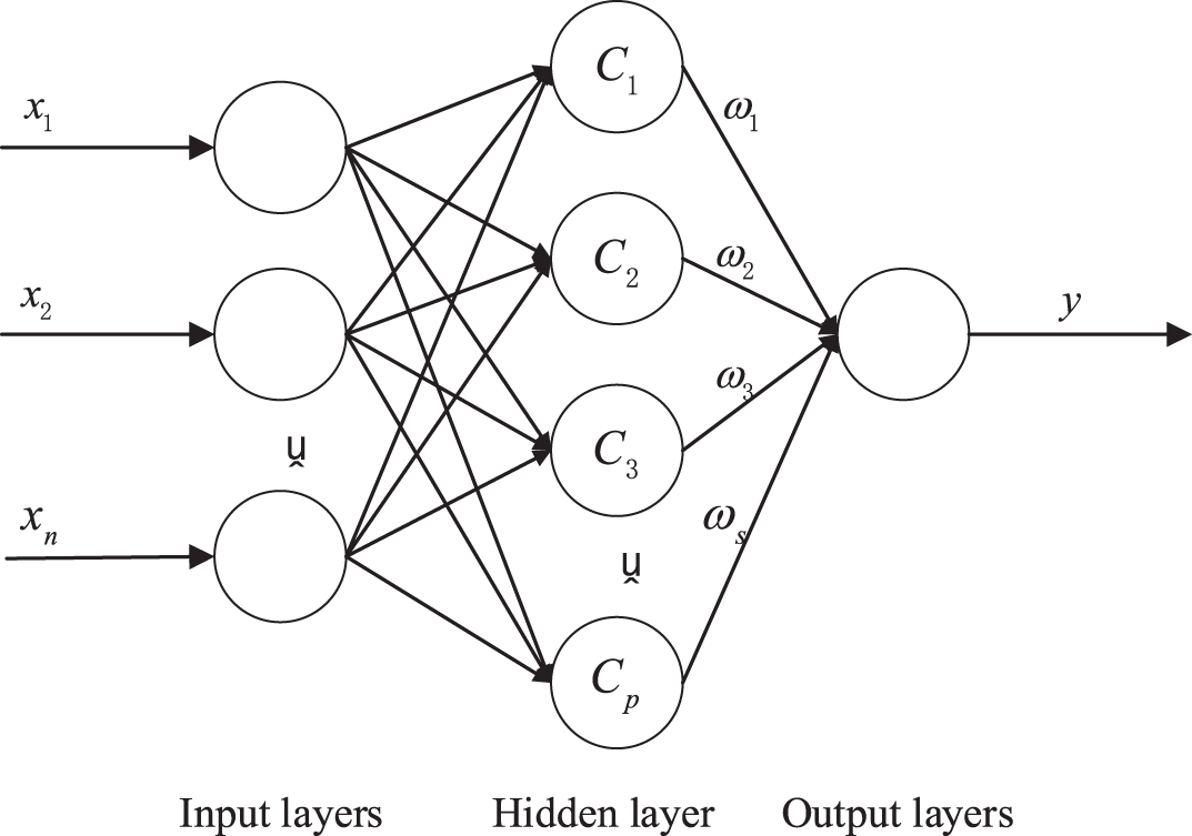
Figure 14: Plot of RBF neural network structure

The input layer is the first step in RBF prediction [18] and is generally selected as the parameter that the neural network needs to train. The hidden layer is the second step of RBF, and a radial basis function is required from the input layer to the hidden layer. The radial basis function is a function of the Euclidean distance from a point in space to a center, which can be a Gaussian kernel function, a quadratic function, or an abnormal S-type function. Due to the better adaptability of Gaussian kernel function to different types of datasets, this article chooses Gaussian kernel function as the radial basis function. Its expression is:

Zi(x)=exp⁡(−12σi2||x−Ci||2),i=1,2,…,p(9)

In the formula: x is the input matrix; Ci is the center of the inth basis function; σi is the variance of the ith Gaussian function; x−Ci is the Euclidean distance between x and Ci, which is a nonlinear transformation. The output layer is the third step of RBF prediction, which assigns different weights to the output values of the hidden layer. Therefore, this process is a linear transformation. The output result of the RBF neural network is obtained through the non-linear transformation from the input layer to the hidden layer and the linear transformation from the hidden layer to the output layer.

5.3 WOA-RBF Algorithm

This article combines the advantages of good optimization performance of WOA algorithm and fewer adjustable parameters of RBF algorithm as an estimation method for battery SOH. Specifically, the extracted five health features and the actual capacity will be used as inputs and outputs for the algorithm, and the dataset will be divided. Using the RBF algorithm as the estimation subject, optimize the extension speed of the radial basis function in the RBF algorithm using the WOA algorithm, and use the root mean square error as the fitness function of the WOA algorithm. The parameters of the WOA algorithm are set to a population of 10, a maximum number of iterations of 20, and a dimension of 1. The radial basis function expansion speed in RBF is optimized by the WOA algorithm. Fig. 15 shows the flowchart of the WOA-RBF algorithm. Table 2 shows the parameter settings for the WOA-RBF algorithm.

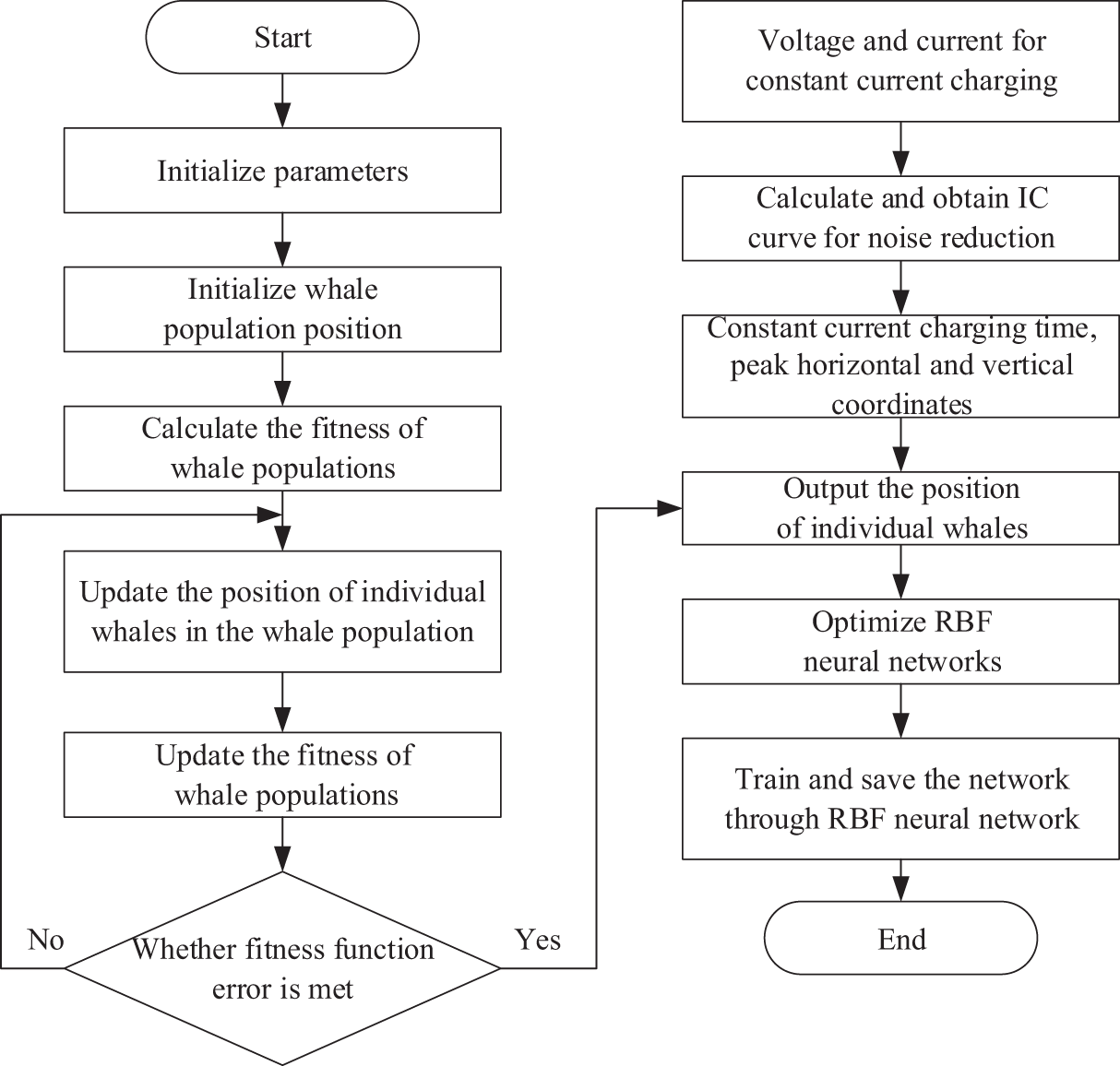
Figure 15: Flow plot of WOA-RBF algorithm

6  Result Analysis

To verify the superiority of the WOA-RBF algorithm proposed in this article, LSTM, RBF, and PSO-RBF algorithms will be used to compare the predicted SOH results with them. Take the five features extracted in the previous text as inputs for these four models, and the actual SOH value of the battery as output. Select 70% of the data as training samples and 30% of the data as test samples to construct four neural network models to compare their predictive performance.

From the prediction results, it can be seen that the model trained by WOA-RBF has better performance and higher prediction accuracy. Fig. 16 shows the prediction results of battery SOH. From the prediction results, it can be seen that the WOA-RBF algorithm’s prediction curve is more in line with the actual curve; Fig. 17 shows the linearity analysis graph. It can be seen from the graph that the WOA-RBF algorithm is closer to the 45° line compared to the other three algorithms, and the convergence speed of this curve is faster than the other three algorithms from the beginning.

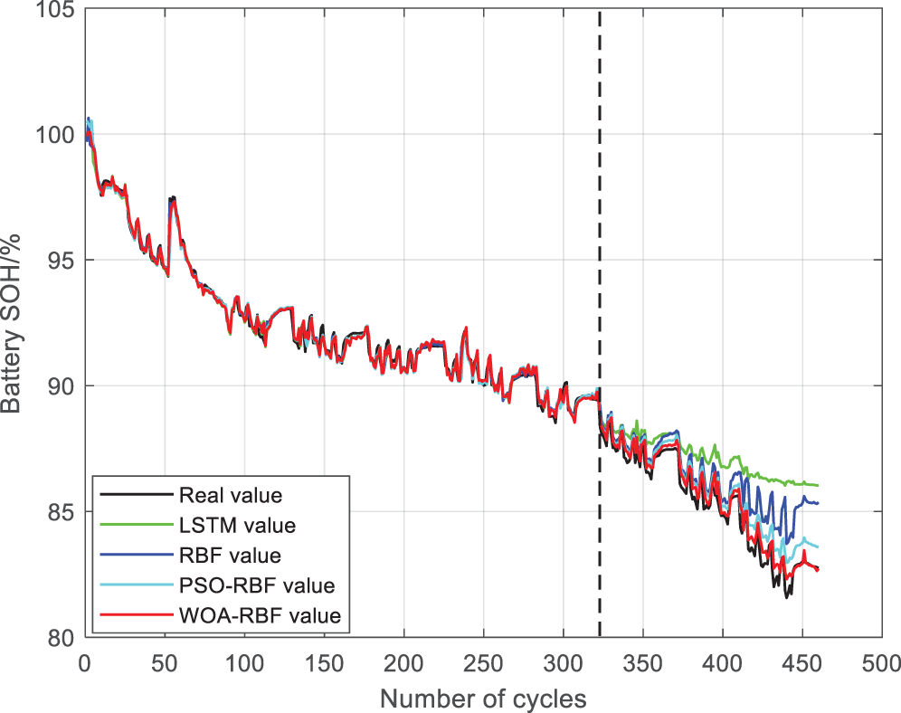
Figure 16: Prediction plots of four algorithms

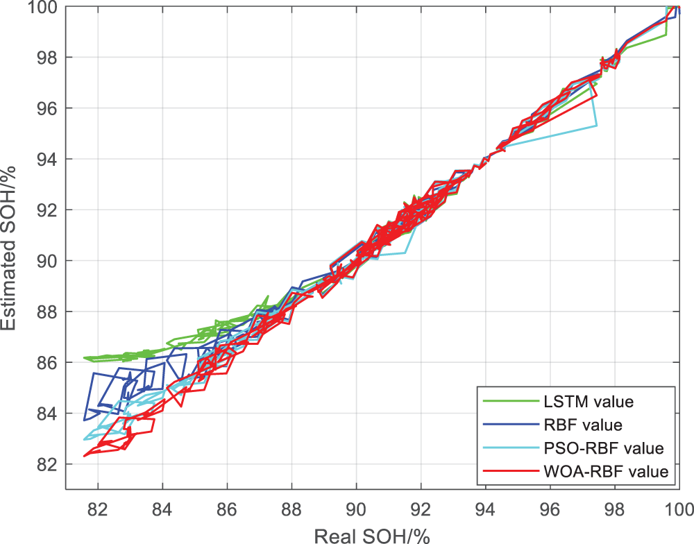
Figure 17: Linearity analysis plots of four algorithms

Fig. 18 shows the absolute error chart. From the absolute error chart, the LSTM algorithm can control the absolute error within 5%, the RBF algorithm can control the absolute error within 4%, the PSO-RBF algorithm can control the absolute error within 2%, and the WOA-RBF algorithm can control the absolute error within 1%; Fig. 19 shows the relative error chart. From the relative error chart, the relative error of LSTM algorithm can be controlled within 6%, RBF algorithm can be controlled within 5%, PSO-RBF algorithm can be controlled within 3%, and WOA-RBF algorithm can be controlled within 2%. Therefore, the WOA-RBF algorithm can train a better model for the extracted feature features, which has high accuracy in predicting battery SOH. Based on the analysis results of the comprehensive algorithm prediction chart, linearity chart, absolute error chart, and relative error chart, it can be concluded that the WOA-RBF algorithm has higher prediction accuracy and convergence speed.

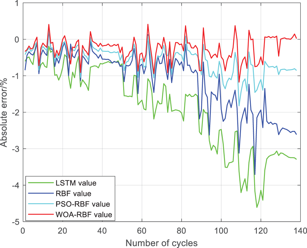
Figure 18: Absolute error plots of four algorithms

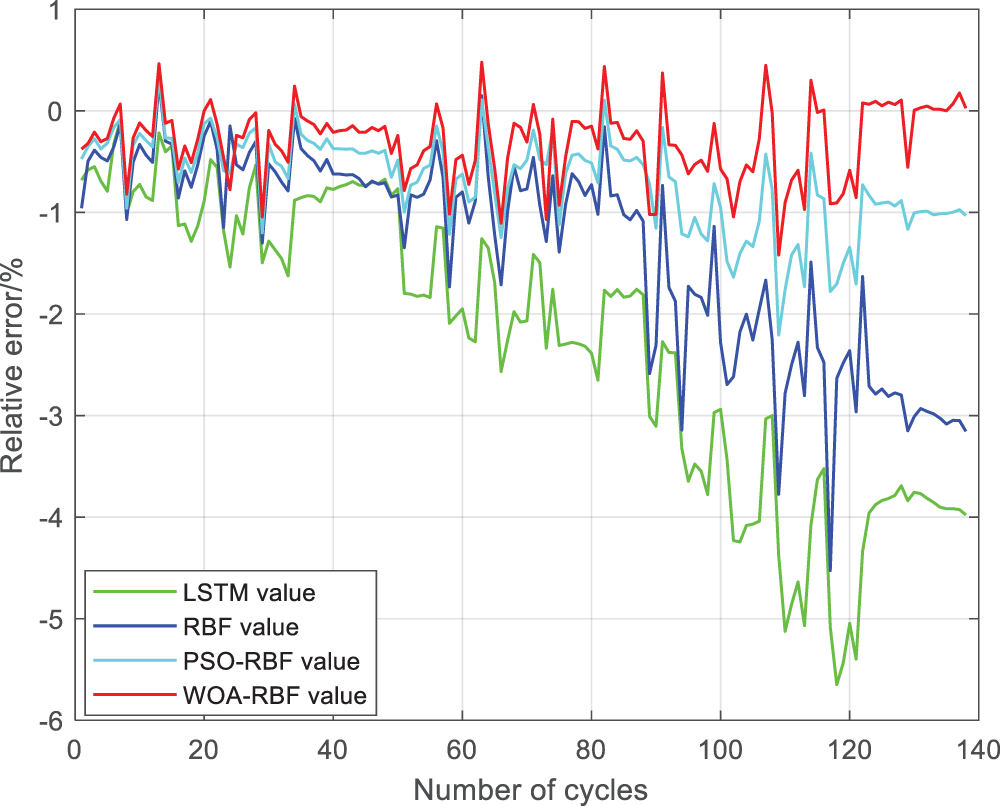
Figure 19: Relative error plots of four algorithms

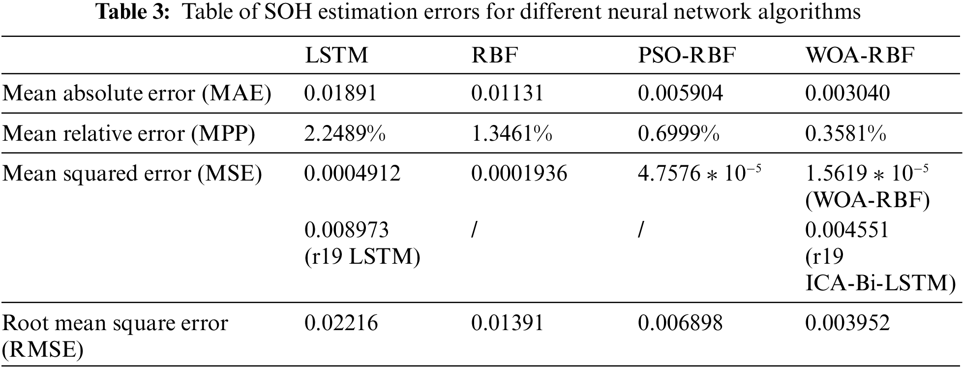
Table 3 shows the SOH estimation error tables of different neural network algorithms, quantitatively comparing the accuracy of the four algorithms from four aspects: average absolute error, average relative error, mean square error, and root mean square error. From the table, it can be seen that the four types of errors of the WOA-RBF algorithm are the smallest, so among the four neural network algorithms, the WOA-RBF algorithm has the highest estimation accuracy. At the same time, Table 3 introduces a comparison with other literature’s SOH estimation results. The mean squared error of SOH estimation in Reference [19] (abbreviated as r19 in the table) is greater than that in this paper, further indicating that the algorithm proposed in this paper has good estimation performance.

7  Extensive Research

This paper selects the CS2-36 dataset as the detailed research object for battery SOH estimation, and also conducts preliminary exploration on the CS2-35, CS2-37, and CS2-38 datasets. The four datasets were collected from batteries of the same model through the same experimental process. The capacity decline curves of the four datasets are shown in Fig. 20. There are outlier points in each dataset in the figure, and the data processing method described in this paper can be used to remove outlier data and extract features. In addition, all four datasets have the same downward trend, which is closely related to the accurate estimation of battery SOH. Therefore, based on the above viewpoints, it can be predicted that using the estimation process and ICA-WOA-RBF algorithm in this paper, good SOH estimation results can be achieved on the CS2-35, CS2-37, and CS2-38 datasets.

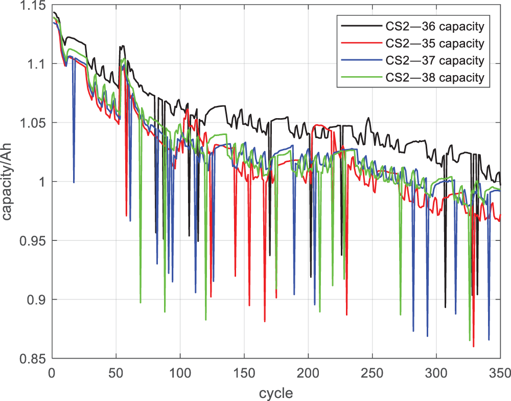
Figure 20: Capacity decline curves of four datasets

8  Conclusion

This article extracts the capacity of battery data, obtains the IC curve and denoises it. Pearson analysis method is used to analyze the correlation, and five features with high correlation with battery SOH are extracted. Four algorithms are used to train the five feature data, and the following conclusions are obtained:

(1) The features extracted by the battery constant current charging time and ICA curve method can establish a good correlation with the battery SOH, which can be better applied to battery SOH estimation;

(2) From a macro perspective, the estimation results of the four algorithms show that the WOA-RBF algorithm is closer to the true curve compared to other algorithms, and its linearity curve is closer to the 45° line;

(3) From a microscopic perspective, the estimation results of the four algorithms show that the WOA-RBF algorithm has lower absolute error, relative error, and faster convergence speed compared to other algorithms;

(4) By displaying the capacity decline curves of the four datasets, it is preliminarily concluded that the method proposed in this paper can still achieve good results in estimating the other three datasets.

Acknowledgement: Acknowledging the contribution of CALCE, University of Maryland, for providing authentic and valuable battery experimental data. Acknowledging Jiangsu University of Technology for providing a stable working environment. Acknowledging all authors for collaborating to complete this article.

Funding Statement: This research was funded by the Basic Science (Natural Science) Research Project of Colleges and Universities in Jiangsu Province, grant number 22KJD470002.

Author Contributions: Qi Wang has completed the testing of the article results and provided financial support; Yandong Gu has completed the simulation in the article and wrote the article; Tao Zhu has completed the verification work of the article; Lantian Ge and Yibo Huang have completed the formatting of the references. All authors reviewed the results and approved the final version of the manuscript.

Availability of Data and Materials: Data openly available in a public repository. The data that support the findings of this study are openly available in CALCE at University of Maryland.

Ethics Approval: Not applicable.

Conflicts of Interest: The authors declare that they have no conflicts of interest to report regarding the present study.

References

1. S. Sun, J. Z. Sun, Z. L. Wang, Z. Y. Zhou, and W. Cai, “Prediction of battery SOH by CNN-BiLSTM network fused with attention mechanism,” Energies, vol. 15, no. 12, Jun. 2022, Art. no. 4428. doi: 10.3390/en15124428. [Google Scholar] [CrossRef]

2. J. Obregon, Y. R. Han, C. W. Ho, D. Mouraliraman, and C. W. Lee, “Convolutional autoencoder-based SOH estimation of lithium-ion batteries using electrochemical impedance spectroscopy,” J. Energy Storage, vol. 60, Mar. 2023, Art. no. 106680. doi: 10.1016/j.est.2023.106680. [Google Scholar] [CrossRef]

3. S. M. Qaisar and A. E. E. AbdelGawad, “Prediction of the li-ion battery capacity by using event-driven acquisition and machine learning,” presented at the 2021 7th Int. Conf. on Event-Based Control, Commun., and Signal Process. (EBCCSP), Krakow, Poland, Jun. 22–25, 2021, pp. 1–6. [Google Scholar]

4. Y. Q. Liu, W. J. Lei, Q. Liu, Y. C. Gao, and M. Dong, “Joint state estimation of lithium-ion batteries based on dual adaptive extended particle filters,” (in Chinese), J. Electr. Eng., vol. 39, no. 2, pp. 607–616, Jan. 2024. [Google Scholar]

5. C. X. Yao, X. Li, and L. K. Xing, “Online parameter identification and SOC and SOH estimation based on multi time scale lithium batteries,” (in Chinese), J. Chongqing Univ. of Bus. and Technol. (Nat. Sci. Ed.), vol. 40, no. 5, pp. 48–54, Sep. 2023. [Google Scholar]

6. D. H. Chen, C. Yang, and F. L. Qiu, “Lithium ion battery SOH prediction based on SR-UKF algorithm,” (in Chinese), Modern Electron. Technol., vol. 45, no. 18, pp. 117–121, Sep. 2022. [Google Scholar]

7. J. Y. Zhao, L. R. Huang, and S. L. Yao, “Health state estimation method for lithium-ion batteries considering capacity regeneration,” (in Chinese), J. Power Supply, pp. 1–14, Dec. 2023. [Google Scholar]

8. S. C. Huang, K. H. Tseng, J. W. Liang, C. L. Chang, and M. G. Pecht, “An online SOC and SOH estimation model for lithium-ion batteries,” Energies, vol. 10, no. 4, May 2017, Art. no. 512. doi: 10.3390/en10040512. [Google Scholar] [CrossRef]

9. U. Yayan, A. T. Arslan, and H. Yucel, “A novel method for SoH prediction of batteries based on stacked LSTM with quick charge data,” Appl. Artif. Intell., vol. 35, no. 6, pp. 421–439, May 2021. doi: 10.1080/08839514.2021.1901033. [Google Scholar] [CrossRef]

10. C. L. Zhang, S. S. Zhao, Z. Yang, and Y. Chen, “A reliable data-driven state-of-health estimation model for lithium-ion batteries in electric vehicles,” Front. Energy Res., vol. 10, Sep. 2022, Art. no. 1013800. doi: 10.3389/fenrg.2022.1013800. [Google Scholar] [CrossRef]

11. C. P. Lin, J. Xu, M. J. Shi, and X. S. Mei, “Constant current charging time based fast state-of-health estimation for lithium-ion batteries,” Energy, vol. 247, Mar. 2022, Art. no. 123556. doi: 10.1016/j.energy.2022.123556. [Google Scholar] [CrossRef]

12. S. K. Fu, Y. Z. Wu, R. D. Wang, and M. Z. Mao, “A bearing fault diagnosis method based on wavelet denoising and machine learning,” Appl. Sci., vol. 13, no. 10, Oct. 2023, Art. no. 5936. doi: 10.3390/app13105936. [Google Scholar] [CrossRef]

13. W. Liu, Z. Gou, F. Jiang, G. Liu, D. Wang and Z. Ni, “Improved WOA and its application in feature selection,” PLoS One, vol. 17, no. 5, May 2022, Art. no. e0267041. doi: 10.1371/journal.pone.0267041. [Google Scholar] [PubMed] [CrossRef]

14. J. Nasiri and F. M. Khiyabani, “A whale optimization algorithm (WOA) approach for clustering,” Cogent Math. Stat., vol. 5, no. 1, Jan. 2018, Art. no. 1483565. doi: 10.1080/25742558.2018.1483565. [Google Scholar] [CrossRef]

15. H. Mohammed and T. Rashid, “A novel hybrid GWO with WOA for global numerical optimization and solving pressure vessel design,” Neural Comput. Appl., vol. 32, no. 18, pp. 14701–14718, Mar. 2020. doi: 10.1007/s00521-020-04823-9. [Google Scholar] [CrossRef]

16. A. Kaveh and M. R. Moghaddam, “A hybrid WOA-CBO algorithm for construction site layout planning problem,” Sci. Iran., vol. 25, no. 3, pp. 1094–1104, Aug. 2018. doi: 10.24200/sci.2017.4212. [Google Scholar] [CrossRef]

17. H. Feng et al., “A new adaptive sliding mode controller based on the RBF neural network for an electro-hydraulic servo system,” ISA Trans., vol. 129, pp. 472–484, Jan. 2022. doi: 10.1016/j.isatra.2021.12.044. [Google Scholar] [PubMed] [CrossRef]

18. P. Sohrabi, B. J. Shokri, and H. Dehghani, “Predicting coal price using time series methods and combining of radial basis function (RBF) neural network with time series,” Miner. Econ., vol. 36, no. 2, pp. 207–216, Nov. 2023. doi: 10.1007/s13563-021-00286-z. [Google Scholar] [CrossRef]

19. H. L. Sun, J. R. Sun, K. Zhao, and L. C. Wang, “Data-driven ICA-Bi-LSTM-combined lithium battery SOH estimation,” Math. Probl. Eng., vol. 2022, pp. 1–8, Mar. 2022. doi: 10.1155/2022/9645892. [Google Scholar] [CrossRef]